Sep 1, 2009 - Simulated search-and-rescue is an increasingly popular academic disci- pline worldwide ..... different classes, given a finite set of training data.
Machine Learning Applied to Object Recognition in Robot Search and Rescue Systems
Helen Flynn Keble College University of Oxford
A dissertation submitted for the degree of Master of Computer Science September 2009
Abstract
Recent advances in robotics mean that it is now possible to use teams of robots for many real-world applications. One very important application is robotic search-and-rescue. Robots are highly suitable for search-andrescue scenarios since they may be deployed in highly dangerous environments without putting human responders at risk. Simulated search-and-rescue is an increasingly popular academic discipline worldwide, being a cheaper alternative to using real robots. A highfidelity simulator, USARSim, is used to simulate the environment and its physics, including all robots and sensors. Consequently researchers need not be concerned with hardware or low-level control. The real focus is on improving robot intelligence in such areas as exploration and mapping. In this dissertation, we describe the development of an object recognition system for simulated robotic search-and-rescue, based on the algorithm of Viola and Jones. After an introduction to object recognition and our implementation of a boosted cascade of classifiers for detection, we describe how we integrate our real-time object detection system into robotic mapping. Work so far has focused on victims’ heads (frontal and profile views) as well as common objects such as chairs and plants. We compare the results of our detection system with those of USARSim’s existing simulated victim sensor, and discuss the relevance of our system to real search-and-rescue robot systems. The results of this project will be presented at the 2009 IEEE International Conference on Intelligent Robots and Systems, and published in the proceedings.
Acknowledgements
Sincere thanks go to my project supervisor, Dr. Stephen Cameron, who always had time for me, and whose expert advice proved invaluable not only during the writing of this dissertation, but throughout my year in Oxford. Stephen often went out of his way to assist me in various aspects of the project, and was instrumental in securing funding for my trips to RoboCup events during the year. I am equally indebted to Julian de Hoog for providing guidance on the structure of my project from the very beginning, as well as dealing with any software-related problems I had. Julian always had useful advice to offer me, even when I didn’t ask for it. His enthusiasm for his subject kept this project exciting right to the end. Most of all, I owe heartfelt thanks to my parents who have been a wonderful source of encouragement and support throughout the past year. Without their support I would not be in Oxford, let alone have completed this project. Thank you! Helen Flynn Oxford, 1st September, 2009
Contents 1 Introduction 1.1 Motivation . . . . . . . . . . . . . . . . . . . . . . . . . . . . . . . . . 1.2 Objectives . . . . . . . . . . . . . . . . . . . . . . . . . . . . . . . . . 1.3 Dissertation structure . . . . . . . . . . . . . . . . . . . . . . . . . . .
1 1 2 2
2 Robotic Search and Rescue 2.1 The advantages of robots . . . . . . . . . . . . . 2.2 A brief history of robotic search and rescue . . . 2.2.1 Japan . . . . . . . . . . . . . . . . . . . 2.2.2 United States . . . . . . . . . . . . . . . 2.3 RoboCup Rescue . . . . . . . . . . . . . . . . . 2.3.1 RoboCup . . . . . . . . . . . . . . . . . 2.3.2 Rescue Robots League . . . . . . . . . . 2.3.3 Virtual Robots Competition . . . . . . . 2.3.4 Amsterdam-Oxford Joint Rescue Forces 2.3.5 The USARSim simulator . . . . . . . . .
. . . . . . . . . .
4 4 4 5 5 7 7 7 8 8 9
. . . . . . . . . . .
10 10 11 14 15 16 18 19 20 20 21 22
4 Object Detection Using a Boosted Cascade of Decision Trees 4.1 The frequency transform of an image . . . . . . . . . . . . . . . . . . 4.1.1 Features versus pixels . . . . . . . . . . . . . . . . . . . . . . . 4.1.2 Image transforms . . . . . . . . . . . . . . . . . . . . . . . . .
23 23 23 23
3 The 3.1 3.2 3.3 3.4 3.5 3.6
General Problem of Object Recognition Challenges in object recognition . . . . . . . . A brief history of object recognition . . . . . . The statistical viewpoint . . . . . . . . . . . . Bag of features models . . . . . . . . . . . . . Part-based models . . . . . . . . . . . . . . . Classifier-based models . . . . . . . . . . . . . 3.6.1 Boosting . . . . . . . . . . . . . . . . . 3.6.2 Nearest neighbour methods . . . . . . 3.6.3 Support Vector Machines . . . . . . . . 3.6.4 Neural Networks . . . . . . . . . . . . 3.7 Summary . . . . . . . . . . . . . . . . . . . .
i
. . . . . . . . . . .
. . . . . . . . . .
. . . . . . . . . . .
. . . . . . . . . .
. . . . . . . . . . .
. . . . . . . . . .
. . . . . . . . . . .
. . . . . . . . . .
. . . . . . . . . . .
. . . . . . . . . .
. . . . . . . . . . .
. . . . . . . . . .
. . . . . . . . . . .
. . . . . . . . . .
. . . . . . . . . . .
. . . . . . . . . .
. . . . . . . . . . .
. . . . . . . . . .
. . . . . . . . . . .
. . . . . . . . . .
. . . . . . . . . . .
. . . . . . . . . .
. . . . . . . . . . .
4.2
4.3 4.4
4.5 4.6 4.7 4.8
Haar wavelets . . . . . . . . . . . . . . . . . . . . . . . . 4.2.1 Haar coefficients . . . . . . . . . . . . . . . . . . 4.2.2 Haar scale and wavelet functions . . . . . . . . . 4.2.3 Computational complexity of the Haar transform A fast convolution algorithm . . . . . . . . . . . . . . . . Integral Image . . . . . . . . . . . . . . . . . . . . . . . . 4.4.1 The basic feature set . . . . . . . . . . . . . . . . 4.4.2 An extended feature set . . . . . . . . . . . . . . Dimensionality reduction . . . . . . . . . . . . . . . . . . 4.5.1 Boosting . . . . . . . . . . . . . . . . . . . . . . . Using a cascade of classifiers . . . . . . . . . . . . . . . . Complexity of the Viola Jones Detector . . . . . . . . . . Why Viola and Jones’ algorithm was used in this project
. . . . . . . . . . . . .
. . . . . . . . . . . . .
. . . . . . . . . . . . .
. . . . . . . . . . . . .
5 Training Detectors for Objects in Urban Search and Rescue 5.1 OpenCV software . . . . . . . . . . . . . . . . . . . . . . . . . . 5.2 The training set . . . . . . . . . . . . . . . . . . . . . . . . . . . 5.2.1 Choice and collection of training examples . . . . . . . . 5.2.2 Annotating the images . . . . . . . . . . . . . . . . . . . 5.2.3 Preparing the images for training . . . . . . . . . . . . . 5.3 The training process . . . . . . . . . . . . . . . . . . . . . . . . 5.3.1 Initial hurdles . . . . . . . . . . . . . . . . . . . . . . . . 5.3.2 Parallel machine learning . . . . . . . . . . . . . . . . . . 5.4 Results . . . . . . . . . . . . . . . . . . . . . . . . . . . . . . . . 5.4.1 Receiver Operating Characteristic (ROC) curves . . . . . 5.4.2 Cascade structure . . . . . . . . . . . . . . . . . . . . . . 5.4.3 Features found . . . . . . . . . . . . . . . . . . . . . . . 5.5 Discussion . . . . . . . . . . . . . . . . . . . . . . . . . . . . . . 5.5.1 Insights gained on how to train the best classifiers . . . . 6 Integrating Object Detection into Robotic Mapping 6.1 An introduction to robotic mapping . . . . . . . . . . . . . 6.1.1 The mapping algorithm of the Joint Rescue Forces 6.2 Implementing real-time object detection . . . . . . . . . . 6.3 Improving detection performance . . . . . . . . . . . . . . 6.3.1 Scale factor . . . . . . . . . . . . . . . . . . . . . . 6.3.2 Canny edge detector . . . . . . . . . . . . . . . . . 6.3.3 Minimum number of neighbouring detections . . . . 6.4 Localising objects . . . . . . . . . . . . . . . . . . . . . . . 6.4.1 Estimating the distance to an object . . . . . . . . 6.4.2 Calculating the relative position of an object . . . . 6.4.3 Calculating the global position of an object . . . . 6.5 Multiple detections of the same object . . . . . . . . . . .
ii
. . . . . . . . . . . .
. . . . . . . . . . . .
. . . . . . . . . . . .
. . . . . . . . . . . . .
. . . . . . . . . . . . . .
. . . . . . . . . . . .
. . . . . . . . . . . . .
. . . . . . . . . . . . . .
. . . . . . . . . . . .
. . . . . . . . . . . . .
24 24 25 26 28 29 29 32 32 33 35 36 36
. . . . . . . . . . . . . .
37 37 38 38 40 40 41 44 46 47 47 49 50 51 51
. . . . . . . . . . . .
52 52 53 54 55 55 56 57 57 57 59 59 60
6.6 6.7 6.8 6.9
Improving position estimates by triangulation . . . . Increasing the distance at which objects are detected Results . . . . . . . . . . . . . . . . . . . . . . . . . . Discussion . . . . . . . . . . . . . . . . . . . . . . . .
. . . .
61 62 63 64
7 Conclusions 7.1 Contribution to urban search and rescue . . . . . . . . . . . . . . . . 7.2 Directions for future work . . . . . . . . . . . . . . . . . . . . . . . . 7.3 Concluding remarks . . . . . . . . . . . . . . . . . . . . . . . . . . . .
66 66 67 68
A USARCommander source code A.1 camerasensor.vb . . . . . . . . . . . . . . . . . . . . . . . . . . . . . .
75 75
B OpenCV source code B.1 Code added to cvhaartraining.cpp . . . . . . . . . . . . . . . . . . . .
81 81
C XML detector sample C.1 Left face detector (one stage only) . . . . . . . . . . . . . . . . . . . .
82 82
References
86
iii
. . . .
. . . .
. . . .
. . . .
. . . .
. . . .
. . . .
. . . .
List of Figures 2.1 2.2 2.3
Robots developed as part of the Japanese government’s DDT project. A plywood environment used in the Rescue Robots League. . . . . . . A real Kenaf rescue robot, along with its USARSim equivalent. . . .
6 8 9
3.1 3.2
An exaggerated example of intra-class variation among objects. . . . Fischler and Elschlager’s pictorial structure model . . . . . . . . . . .
11 13
4.1 4.2 4.3 4.4 4.5 4.6
Haar scale and wavelet functions. . . . . . 2D Haar basis functions. . . . . . . . . . . Convolution using the algorithm of Simard Rectangle Haar-like features. . . . . . . . . Computing the integral image. . . . . . . . Extended set of Haar features. . . . . . . .
26 27 29 30 31 32
5.1 5.2 5.3 5.4 5.5 5.6 5.7 5.8 5.9
Positive training examples. . . . . . . . . . . . . . . . . . . . . . . . . The Createsamples utility. . . . . . . . . . . . . . . . . . . . . . . . . The Haartraining utility. . . . . . . . . . . . . . . . . . . . . . . . . . Training progress. . . . . . . . . . . . . . . . . . . . . . . . . . . . . . Summary of classifier performance. TP=true positive, FP=false positive. Sample images of objects detected. . . . . . . . . . . . . . . . . . . . ROC curves. . . . . . . . . . . . . . . . . . . . . . . . . . . . . . . . . Real people detection. . . . . . . . . . . . . . . . . . . . . . . . . . . First two features selected by AdaBoost. . . . . . . . . . . . . . . . .
39 41 43 44 47 48 49 49 50
6.1 6.2 6.3 6.4 6.5 6.6 6.7 6.8
A map created during a run in USARSim. . . . . . . . . . . . Visual Basic code for detection objects in an image. . . . . . . The USARCommander interface. . . . . . . . . . . . . . . . . Calculating an object’s angular size. . . . . . . . . . . . . . . . Calculating angular offset of an object. . . . . . . . . . . . . . Triangulation. . . . . . . . . . . . . . . . . . . . . . . . . . . . A completed map with attributes. . . . . . . . . . . . . . . . . Comparing our face detector with USARSim’s victim detector.
53 55 56 58 59 61 62 63
iv
. . . . . . et al. . . . . . . . . .
. . . . . .
. . . . . .
. . . . . .
. . . . . .
. . . . . .
. . . . . .
. . . . . .
. . . . . .
. . . . . .
. . . . . . . .
. . . . . .
. . . . . . . .
. . . . . .
. . . . . . . .
. . . . . .
. . . . . . . .
List of Tables 4.1 4.2 4.3
Computing the Haar transform. . . . . . . . . . . . . . . . . . . . . . Number of features inside a 24 × 24 sub-window. . . . . . . . . . . . Viola and Jones’ complete learning algorithm. . . . . . . . . . . . . .
25 33 34
5.1 5.2 5.3
Number of training examples used for our classifiers. . . . . . . . . . Approximate training times for our classifiers, using the OSC. . . . . Number of Haar features used at each stage of our face classifier. . . .
38 47 50
v
Chapter 1 Introduction Recent advances in technology and computer science mean that it is now possible to use teams of robots for a much wider range of tasks than ever before. These tasks include robotic search and rescue in large scale disasters, underwater and space exploration, bomb disposal, and many other potential uses in medicine, the army, domestic households and the entertainment industry. Robotic search and rescue has become a major topic of research, particularly since the terrorist attacks of September 2001 in New York. Robots are highly suitable for search-and-rescue tasks like this since they may be deployed in dangerous and toxic environments without putting human rescue workers at risk. While much effort has gone into the development of robust and mobile robot platforms, there is also a need to develop advanced methods for robot intelligence. Specific intelligence-related areas include exploration, mapping, autonomous navigation, communication and victim detection. This project investigates the application of machine learning techniques to object recognition in robotic search-and-rescue. In particular, a boosted cascade of decision trees is chosen to detect various objects in search-and-rescue scenarios. The highfidelity simulator, USARSim, which has highly realistic graphical rendering, is used as a testbed for these investigations.
1.1
Motivation
Since the primary goal of robotic search and rescue is to find victims, a simulated robot rescue team must also be able to complete this task. In real rescue systems, identification of victims is often performed by human operators watching camera feedback. It would be desirable to have a more realistic simulation of real-world victim detection, whereby robots can automatically recognise victims using visual information, and put these into a map. Although other advanced systems exist to detect specific characteristics of human bodies, such as skin colour, motion, IR signals, temperature, voice signals and CO2 emissions, these systems can be expensive, especially where there are teams of robots. Cameras are a cheaper alternative which can be 1
attached to most robots. A secondary goal of search and rescue efforts is to produce high quality maps. One of the reasons to generate a map is to convey information, and this information is often represented as attributes on a map. In addition to victim information, useful maps contain information on the location of obstacles or landmarks, as well as the paths that the individual robots took. Machine learning techniques provide robust solutions to distinguishing between different classes, given a finite set of training data. This makes them highly applicable to object recognition where object categories have different appearances under large variations in the observation conditions. This project aims to demonstrate the applicability of machine learning techniques to automatically recognising and labeling items in search-and-rescue scenarios.
1.2
Objectives
The main objectives of this project were as follows: (1) To investigate whether machine learning techniques might be applied with success to the low resolution simulator images from USARSim; (2) To determine whether object classifiers can be successfully ported to real-time object detection; (3) To demonstrate that visual sensors can be successfully used in conjunction with other, more commonly used perceptual sensors in robotic mapping.
1.3
Dissertation structure
The goal of this project was to develop an understanding of the current state of the art in object recognition, and then to develop our own object detection system based on the learning technique deemed to be the most suitable in terms of recognition accuracy and detection speed. There are two parts to the dissertation: (i) a study of how machine learning techniques have been applied to pattern recognition tasks in the past, and (ii) the implementation and integration of real-time object recognition into robotic mapping. The dissertation is structured as follows: • Chapter 2 - Robotic Search and Rescue - provides a brief history of how robots came to be used in search-and-rescue tasks, the advantages of using robots in such situations, and an overview of the RoboCup competitions used to benchmark the progress of research in this area. • Chapter 3 - The General Problem of Object Recognition - discusses object recognition as a field of computer vision, the challenges faced by recognition systems, 2
a study of the various machine learning techniques that have been applied to object recognition and their suitability for different types of recognition problems. • Chapter 4 - Object Detection Using a Boosted Cascade of Decision Trees describes in detail the object detection algorithm used in this project, its computational complexity and suitability for use in real-time applications. • Chapter 5 - Training Detectors for Objects in Urban Search and Rescue - describes the approach we used to train classifiers to detect objects in urban search and rescue systems, problems encountered along the way, followed by the results obtained. • Chapter 6 - Integrating Object Detection into Robotic Mapping - introduces the topic of robotic mapping, how our object detection system was integrated into robotic mapping, and finally, the results obtained. • Chapter 7 - Conclusions - sums up the contributions of this project and discusses future directions for research in the area of robotic search and rescue.
3
Chapter 2 Robotic Search and Rescue 2.1
The advantages of robots
The use of robots for particular tasks, particularly search and rescue tasks, is desirable for a number of reasons: • Robots are expendable, so they can be deployed in disaster zones where it would be too dangerous for humans to go. They can be designed to cope with excessive heat, radiation and toxic chemicals. • Robots can be made stronger than humans. • Robots may have better perception sensors than humans. Using camera, sonar or laser scanners, robots may be able to learn much more about their environment than a human ever could. • Robots may be more mobile than humans. For example, shoebox-sized robots can fit into places where humans can not, or aerial robots can explore an environment from heights. • Robots can be very intelligent. Intelligent agents and multi-agent systems have become a very active area of research, and it is conceivable that robots will be able to make decisions faster and more intelligently than humans in the near future. This work in this project is concerned primarily with robotic search and rescue, whose main task is to map a disaster zone and to relay as much information as possible to human rescue responders. Useful information might include the location and status of victims, locations of hazards, and possible safe paths to the victims.
2.2
A brief history of robotic search and rescue
The use of robots in search and rescue operations has been discussed in scientific literature since the early eighties, but no actual systems were developed until the 4
mid nineties. In the history of rescue robotics, disasters have been the driving force for advancement. While active research is now being undertaken worldwide, the first proponents of using robots for search and rescue tasks were Japan and the United States.
2.2.1
Japan
The Great Hanshin-Awaji earthquake claimed more than 6,400 human lives in Kobe City on January 17, 1995. This prompted major research efforts towards developing autonomous mobile robots to assist first responders in emergency scenarios. Among the initiatives introduced by the government was a five-year project, the Special Project for Earthquake Disaster Mitigation in Urban Areas. In addition to focussing on geophysical and architectural concerns, much of this project was dedicated to disaster management systems. In this regard, a Special Project on Development of Advanced Robots and Information Systems for Disaster Response, often referred to as the “DDT project”, was set up. This project addressed the following issues [53]: 1. Mobility and information mapping of/by information collection robots aiming at surveillance of disaster field that is inaccessible by human and at enhancement of information collection ability. 2. Intelligent sensors and portable digital assistances for collection and synthesis of disaster damage information. 3. Human interface (both teleoperation and information display) for human users so that robots and systems become useful tools for human. 4. Network-based integration for advanced social infrastructure for disaster response. 5. Performance evaluation of the systems (test field, etc.) and standardisation (network protocol, etc.). This project spawned a national drive towards developing effective search and rescue robots, and a large number of laboratories throughout Japan are now dedicated to the topic. Figure 2.1 shows some robots developed as part of the Japanese government’s DDT project.
2.2.2
United States
The bombing of Oklahoma City in 1995 propelled research into rescue robotics in the U.S. Although robots were not actually used in the response to the bombing, a graduate student and major in the U.S. Army at the time, John Blitch, participated in the rescue effort and took notes as to how robots might have been applied. He observed that no robots of the right size, characteristics or intelligence were available for search and rescue. As a result of his increased interest, Blitch changed the topic 5
(a) Intelligent aero-robot
(b) “Hibiscus”
(c) Helios VIII
Figure 2.1: Robots developed as part of the Japanese government’s DDT project. of his Master’s thesis from planetary rovers to determining which existing robots are useful for particular disaster situations. Blitch’s work provided much of the motivation for the DARPA Tactical Mobile Robot (TMR) program, which developed small robots for military operations in urban terrains. He later became program manager of the DARPA TMR team, which developed many of the robots that were used in the response to the World Trade Center attacks in 2001. Over eleven days in the aftermath of September 11, Blitch’s seven robots squeezed into places where neither humans nor dogs would fit, dug through piles of scalding rubble, and found the bodies of seven victims trapped beneath heaps of twisted steel and shattered concrete. During the later weeks of the recovery, robots were used by city engineers in a structural integrity assessment, finding the bodies of at least three more victims in the process. This was the first deployment of rescue robots ever, and supported Blitch’s ambition “to build robots that can do things human soldiers can’t do, or don’t want to do”. As a result of the exercise, rescue robots gained a much greater profile and acceptance amongst rescue workers. It also gave a better idea of the skills required by both humans and robots for successful rescue efforts, and what areas required urgent attention. A review of the mistakes made during the WTC rescue effort by robots concluded that improvements were needed in the following areas [36]: 1. advanced image processing systems 2. tether management 3. wireless relay 4. size and polymorphism 5. localisation and mapping 6. size and distance estimation 7. assisted navigation In addition to widespread support for rescue robots in the U.S. and Japan, their potential value has now been recognised worldwide. Besides the development of robust mobile robot platforms, robot intelligence is an important area in need of further 6
development. Even a highly sophisticated-looking robot can fail if it cannot make use of sensory information to maximum effect, whilst navigating an environment. Specific intelligence-related areas include exploration, mapping, autonomous navigation, communication and victim detection. Given the costs involved in experimenting with real robots in dangerous environments, there has been an increasing focus on simulation-based research. Currently, the most widely used simulation framework for research into rescue robotics is the USARSim simulator (see Section 2.3.5) which is used in the Virtual Robots Competition of RoboCup Rescue (see Section 2.3.3).
2.3 2.3.1
RoboCup Rescue RoboCup
RoboCup is a international initiative to foster research and education in robotics and artificial intelligence. Begun in 1993, the main focus of RoboCup activities was competitive football. Arguing that the fun and competitive nature of robot soccer can increase student interest in technology and quickly lead to the development of hardware and software applicable to numerous other multi-agent systems domains, RoboCup set itself the goal of “By the year 2050, develop a team of fully autonomous humanoid robots that can win against the human world soccer champion team”. In recent years, RoboCup has branched out into a number of other areas. These include RoboCupJunior, aimed at increasing enthusiasm for technology amongst school children, RoboCup@Home, aimed at developing service and assistive robot technology, and RoboCup Rescue, a collection of competitions related to the development of both hardware and software for the purposes of disaster management and robotic search and rescue. RoboCup Rescue has two main events: the Rescue Robots League and the Virtual Robots Competition.
2.3.2
Rescue Robots League
The Rescue Robots League is concerned with real robots, like those deployed at the World Trade Center in 2001. Competing institutions design complete robot systems. Large plywood-based environments containing obstacles and based on realistic disaster scenarios (according to standards set by the National Institute of Standards and Technology [27]) are populated with dummy victims. Competing teams are required to use their own human-robot interfaces and communication protocols to direct the robots through the environment during a limited period of time. Points are awarded based on map quality, number of victims found and information on their status. Points are deducted if robots collide with the arena or with victims. Figure 2.2 shows an example of a plywood environment used in the Rescue Robots League.
7
Figure 2.2: A plywood environment used in the Rescue Robots League.
2.3.3
Virtual Robots Competition
The Virtual Robots Competition is largely a simulated version of the Rescue Robot League. A high-fidelity simulator, USARSim (see Section 2.3.5), is used to simulate the environment and its physics, including all robots and sensors. This means that participants do not have to deal with hardware issues. Rather, the focus is on highlevel tasks such as multi-agent cooperation, mapping, exploration, navigation, and interface design. Similar to the Rescue Robots League, points are awarded to participants based on the number of victims found, information on the location and status of victims, and quality of the map, including map attribution. Points are deducted if the robot collides with anything, or if there is any human intervention in the rescue effort.
2.3.4
Amsterdam-Oxford Joint Rescue Forces
One of the founding teams of the Virtual Robots competition, UvA Rescue, was developed at the Intelligent Systems Laboratory at the University of Amsterdam. Developing a team for participation in this competition is a very demanding process. In addition to the basics required to operate robots in the environment (user interface, communication, etc.), teams must also implement high-level techniques, including exploration, mapping, autonomous navigation and multi-robot coordination. Development of a fully integrated search-and-rescue team for the competition requires excellent software. UvA Rescue’s software program (henceforth referred to as USARCommander ) was developed using a well-structured modular approach. The team website provides an extensive set of publications which provide detailed information on their approach. In April 2008, Oxford Computing Laboratory joined UvA Rescue and the team was renamed the Amsterdam Oxford Joint Rescue Forces (henceforth referred to as the Joint Rescue Forces). At the annual RoboCup Rescue competition in Suzhou, China in July 2008, the team came seventh, while in this year’s competition in Graz, 8
Austria, the team came third1 out of eleven teams.
2.3.5
The USARSim simulator
USARSim (Urban Search and Rescue Simulator) is an open-source high-fidelity simulator originally developed for the RoboCup Rescue competition in 1999. It is built on top of Unreal Engine 2.0, a commercial game engine produced by Epic Games, which markets first-person shooter games. While the internal structure of the game engine is proprietary, there is an interface called gamebots which allows external applications to interact with the engine. A number of publicly available robot platforms, sensors, and environments have been created for USARSim. The list of available robot platforms (all based on real robots) includes P2DX, P2AT, ATRVJr, AirRobot, TeleMax, Rugbot and Kenaf robots. Available sensors include a state sensor, sonar sensor, laser scanner, odometry sensor, GPS, INS, touch sensor, RFID sensor, camera sensor and an omni-directional camera. More than thirty separate environments have been developed, containing a range of indoor and outdoor scenes with a variety of realistic obstacles and challenges. Figure 2.3 shows an example of a real Kenaf robot, together with its USARSim equivalent.
Figure 2.3: A real Kenaf rescue robot, along with its USARSim equivalent. In addition to its realistic emulation of robot platforms, the high quality visual rendering of USARSim makes it an ideal testbed for object recognition techniques in USAR situations. While the focus of this project is on integrating object recognition into robotic mapping, USARSim is also ideal for the testing of many other intelligencerelated techniques, and provides the impetus to ensure that these techniques work not only in theory but also in practice.
1
Detailed coverage of our team’s performance can be found at http://www.robocuprescue.org/ wiki/index.php?title=VRCompetitions#Competition_Schedule.
9
Chapter 3 The General Problem of Object Recognition The focus of this project was in providing assistance to a human robot operator to recognise victims in simulated camera feeds. This chapter describes object recognition as a problem in itself, and the application of machine learning methods to object recognition. The problem can broadly be divided into generic object recognition and specific object recognition. Generic object recognition attempts to assign objects to general categories, such as faces, cars, plants or furniture. The latter is meant to recognise specific objects like Bill Clinton’s face or the Leaning Tower of Pisa. In either case, various issues must be addressed by the system. The basic question, ‘is the object in the image?’, is a classification problem. Object detection on the other hand answers the question ‘where in the image is the object?’. In this situation, we may not even know if the object is present at all, much less its location in the image. A third problem is to determine the type of scene based on the objects that are present in an image. For instance, a desk, chair and computer might indicate an office environment. In this chapter, we discuss the challenges inherent in object recognition, present a brief history of research in the field, and discuss the role of machine learning in recognising objects.
3.1
Challenges in object recognition
Recognising objects is not an easy task for computers. There are many challenges we all face in recognising objects, and human vision systems deal with them very well. In designing machine learning algorithms for recognition, however, the following challenges must receive special attention: • Viewpoint variation: 3D volumetric objects, when seen from different viewpoints, can render very differently in an image. • Varying illumination: Different sources of illumination can drastically change the appearance of an object. Shadows cast by facial features can transform the 10
face depending on the direction of light, to the point where it is difficult to determine if it is the same person. • Occlusion: Objects don’t exist in the world by themselves in a completely clean and free environment. Usually environments are quite cluttered, and the object is occluded by other objects in the world. Self-occlusion can even occur when dealing with quite articulated objects. • Scale: Objects from the same category can be viewed at very different scales; they might have different physical sizes, or they might be geometrically rendered differently, depending on the distance between the camera and the object. • Deformation: This is a problem particularly for articulated objects, including our own human bodies, animals and ‘stringy’ objects. • Clutter: We would like to be able to pinpoint an object in an image when it is surrounded by a lot of background clutter. The challenge is being able to segment the object from the background. • Intra-class variation: Objects from the same category can look very different to each other (see Figure 3.1). For example, there are many kinds of chairs, each of which looks very different to the next.
Figure 3.1: An exaggerated example of intra-class variation among objects. Given these challenges, computer vision researchers have been faced with a formidable task of getting computers to recognise objects. In the beginning, research focused on single object recognition (recognising a cereal box, say, on a shelf isle), before advancing into methods for generic object class recognition. A brief history now follows.
3.2
A brief history of object recognition
Swain and Ballard [52] first proposed colour histograms as an early view-based approach to object recognition. Given an example image of a object, we can measure 11
the percentage of pixel values1 in different colour bins. Then, when a new example is presented, we can compare its colour histogram with that of previously seen examples. The main drawback of this approach is its sensitivity to lighting conditions, since an object can have a different colour when it is illuminated. Moreover, very few objects can be described by colour alone. Schiele and Crowley [47] extended the idea of histograms to include other local image features such as orientation and gradient magnitude, forming multidimensional histograms. In [34], Linde et al. used more complex descriptor combinations, forming histograms of up to 14 dimensions. Although these methods are robust to changes in rotation, position and deformation, they cannot cope with recognition in a cluttered scene. The issue of where in an image to measure has had an impact on the success of object recognition, and thus the need for ‘object detection’. Global histograms do not work well for complex scenes with many objects. Schneiderman and Kanade [48] were amongst the first to address object categorisation in natural scenes, computing histograms of wavelet transform coefficients over localised parts of an object. Wavelet transforms are used to decompose an image into a collection of salient features while reducing the redundancy of many pixels. In keeping with the histogram approach, the popular SIFT (Scale-Invariant Feature Transform) descriptor [35] uses position-dependent histograms calculated around selected points in the image. In 2006, Herbert et al. [5] introduced the SURF (Speeded Up Robust Features) algorithm, which is a variation of SIFT. It builds upon the strengths of SIFT but simplifies the methods to the absolute essential, resulting in faster computation times. The most complex methods take into consideration the relationship between the parts that make up an object, rather than just its overall appearance. Agarwal et al. [1] presented an approach to detect objects in grey images based on a part-based representation of objects. A vocabulary of object parts is constructed from a set of example images of the object. Images are represented using parts from the vocabulary, together with spatial relations observed between them. This built upon a simple concept of pictorial structure models proposed in the early seventies by Fischler and Elschlager [19]. Their basic idea was to represent an object by a collection of parts in a deformable arrangement (see Figure 3.2). Each part’s appearance was modeled separately, and the whole object was represented by a set of parts with spring-like links between them. These models allowed for qualitative descriptions of an object’s appearance, and were suitable for generic recognition tasks. Face recognition has attracted wide interest since Fischler and Elschlager’s seminal work in the seventies. Turk and Pentland [56] used eigenfaces, a set of digitised pictures of human faces taken under similar lighting conditions, normalised to line up the facial features. Eigenfaces were then extracted out of an image by means of principal components analysis. Rowley et al. [44] proposed an advanced neural network approach for detecting faces, which employed multiple neural networks to classify different facial features, and used a voting system to decide if an entire face 1 Swain and Ballard constrained the pixel values to lie within the range 0 to 255. Zero is black, and 255 is white. Values in between make up the different shades of gray.
12
had been detected. Schneiderman and Kanade [48] described a na¨ıve Bayes classifier to estimate the joint probability of appearance and position of facial features, at multiple resolutions. Assuming statistical independence between the different features, the probability for the whole object being a face is the product of the individual probabilities for each part. More recently, Viola and Jones [58] presented a face detection scheme based on a ‘boosted cascade of simple features’. What set their algorithm apart from previous face detectors was that it was capable of processing images extremely fast in real time. Their algorithm will be discussed in detail in the next chapter.
Figure 3.2: Fischler and Elschlager’s pictorial structure model. Image extracted from [19]. Handwritten digit recognition has also received vast amounts of attention in the computer vision community. Given a set of handwritten digits, the task of a computer is to output the identity of the digit 0, . . . , 9. LeCun et al. [29] experimented with various neural network architectures for optical character recognition, and found that effective classifiers could be built which operate directly on pixels, without the need for feature extraction. However, the success of these methods depended on the characters first being size-normalised and de-slanted. Amit and Geman [3] proposed a digit detector in the style of a degenerate decision tree, in which a large majority of candidate subregions within an image can be discarded early on in the process, leaving only a few regions requiring further processing. They find key points or landmarks, and try to recognise objects using the spatial arrangements of point sets on the boundaries of digits. However, not all characters have distinguishable keypoints (think of the character ‘O’). To deal with issues like this, Belongie et al. [6] presented a simple algorithm for finding correspondences between shapes, which need not depend on characters having inflection points. They introduced a shape descriptor to describe the rough distribution of the rest of the shape with respect to a given point on the shape. Using the matching errors between corresponding points as a gauge of dissimilarity, they used nearest neighbour methods for object recognition.
13
3.3
The statistical viewpoint
Given an image, we want to know whether it contains a particular class of object or not. Using a face as an example this can be viewed as a comparison between two probability scores: (1) the probability that, given an image, it contains a face and (2) the probability that, given an image, it does not contain a face. The question is, given an image, how probable is it that a face is in the image: P (face|image) > P (no face|image) Using Bayes’ rule, this can be expanded to: P (face|image) P (image|face) P (face) = · P (no face|image) P (image|no face) P (no face) | {z } | {z } | {z } posterior ratio
likelihood ratio
prior ratio
The likelihood ratio means, given some model of the object class, what the likelihood of a particular instance is. There are two machine learning techniques that are commonly used to solve the problem of object categorisation - discriminative learning and generative learning. Discriminative learning tends to look at the posterior probability directly and tries to find boundaries between two (or n) classes. It asks the question, ‘given an image, does it contain a face or not?’. Essentially, discriminative learning tries to learn a model that is able to distinguish between positive and negative training examples. Generative learning, on the other hand, tries to model the whole joint distribution of image features: P (x1 , x2 , . . . , xn ). It looks at the likelihood probability, asking the question, ‘given an underlying model for a face, how likely is it that this new image came from that underlying distribution?’. It is hoped that the joint distribution accurately captures the relationships between the variables. This kind of model typically learns by maximising the likelihood of positive training data (images containing the object). From a computational point of view, generative models are considered to be more complex, since they produce a full probability density model over all the image features. Discriminative models merely try to find a mapping from input variables to an output variable, with the goal of discriminating between classes, rather than modeling a full representation of a class. There is therefore no redundancy. In practice, discriminative models produce quite accurate results, and often outperform generative models in the same settings. In designing models for object recognition, the main issues are how to represent an object category, the learning method (how to form a classifier, given training data) and the actual recognition method. The representation can be generative, discriminative or a combination of the two. In choosing a representation, the issue is whether we think an object should be represented solely by its appearance, or by a combination of location and appearance. Ideally, the representation should incorporate techniques for dealing with invariance to lighting, translation, scale and so on. It is also important 14
to look at how flexible the model is; in early face recognition for example, global information was used to describe the whole object, but as researchers became more aware of the challenges in recognition, such as occlusion, eigenfaces were found to be lacking in expressiveness, so localised models were used, which took into account the parts making up an object and how they relate to each other. Object recognition relies on learning ways to find differences between different classes, and this is why machine learning methods have exploded in the field of computer vision. In addition to deciding whether to opt for discriminative or generative models, one also has to decide the level of supervision in learning. For example, when building a classifier for cars, we can supply images of cars on their own, or supply images of cars in a natural scene, and ‘tell’ the algorithm where to find the car by manually tagging it. Alternatively, we could supply the location of the most important car features, such as the wheels, headlights, etc. At the training stage, over-fitting is a major issue, because the classifier could end up learning the noise in images, rather than the general nature of the object category. This is why it is important to supply many images of the objects, which include as many sources of variation as possible. Once the model has been trained, the speed at which an object can be recognised is crucial, because if the system is to be used in real-time applications, recognition must be done quickly. One has to decide whether to search over the whole image space for the object, or to perform a more efficient search over various scales and locations in the image. We now look in more detail at some of the methods introduced above, focusing first on generative models in Sections 3.4 and 3.5, and concluding with a discussion of discriminative methods in Section 3.6.
3.4
Bag of features models
The simplest approach to classifying an image is to treat it as a collection of regions, describing only its appearance and ignoring the geometric relationship between the parts i.e. shape. Most of the early bag of features models were related to the texture of an object. This approach was inspired by the document retrieval community, who can determine the subject or theme of a document by analysing its keywords, without regard to their ordering in a document. Such models are called ‘bag of words’ models, since a document is represented as a distribution over a fixed vocabulary of words. In the visual domain, building blocks of objects, even without any geometric information, can give a lot of meaning to visual objects, just as keywords can give a sense of the type of document. Recently, Fei Fei et al. [16] applied such methods successfully to object recognition. For each object, it is necessary to generate a dictionary of these building blocks and represent each class of objects by the dictionary. One question is how to specify what the building blocks of an object should be. A simple way is to break down the image into a grid of image patches, as in [16, 59]. Alternatively, it is possible to use a more 15
advanced algorithm for determining interest points, like SIFT descriptors by Lowe [35] or a speeded up version of this algorithm called SURF [5]. The interest points found must then be represented numerically, in order to pass them to a learning algorithm. They could be represented by wavelet functions, or just by their pixel intensity. In either case, the regions are expressed as vectors of numbers and there are typically thousands of them. With thousands of interest points identified, it is necessary to group them together in order to have ‘building blocks’ which can be universally used for all the images. The simplest way to do this is to cluster the interest points. The result is, say, a couple of hundred building blocks for an object, given several thousand original vectors of interest points. It is then necessary to represent the image by the building blocks. This is done by analysing an image and counting how many of each building block is in the image. This histogram of the dictionary becomes the representation of the image. Popular algorithms which implement the bag of words model are na¨ıve Bayes classifiers [13] and hierarchical bayesian models [50]. Once the model has been formulated, the actual recognition process involves representing a new image as a bag of features, matching it with the category model, and then selecting the most probable category. Scale and rotation are not explicitly modeled in bag of features models, but they are implicit through the image descriptors. The model is relatively robust to occlusion, because it is not necessary to have an entire image to determine if an object is present, as long as there are enough patches to represent the object category. Bag of features models do not have a translation issue at all. The main weakness of the model is its lack of shape information. It is also unclear as yet how to use the model for segmenting the object from its background. A bag of features model captures information not only about the object of interest, but also contextual information (background). This might be useful in recognising some object categories, given that certain objects are only likely to appear in certain contexts; however, the danger is that system may fail to recognise the object from the background and show poor generalisation to other environments.
3.5
Part-based models
A part-based model overcomes some of the deficiencies of a bag of features model because it takes into account the spatial relationship between the different parts of an object. Although instances belonging to a general category of objects have dissimilarities, they also share many commonalities. In cars, for example, the headlights are very similar, as are the wheels and wing mirrors. Not only are they similar in appearance, but they are also similar in their arrangement relative to each other. The idea behind a part-based model is to represent an object as a combination of its appearance and the geometric relationship between its parts. This representation, which encodes information on both shape and appearance, is called a constellation model, first introduced by Burl [10] and developed further by Weber [60] and Fergus 16
[18]. As in bag of features models, feature extraction algorithms like SIFT and SURF can be used to identify the important structures in images, while de-emphasising unimportant parts. The process of learning an object class involves first determining the interesting features and then estimating model parameters from these features, so that the model gives a maximum likelihood description of the training data. The simplest way to model this is with a Gaussian distribution where there is a mean location for each part and an allowance for how it varies. Precisely, each part’s appearance is represented as a point in some appearance space. The shape (how parts are positioned relative to one another) can also represented by a joint Gaussian density of the feature locations within some hypothesis. An object is then represented as a set of regions, with information on both appearance and geometric information (shape). For a 100 × 100 pixel image, there would typically be around 10-100 parts [17]. The advantage of a part-based model, then, is that is computationally easier to deal with a relatively small number of parts than the entire set of pixels. However, a major drawback of the part-based approach is that it is rather sparse; since it focuses on small parts of the image, the model doesn’t quite express the object in its entirety. It can be difficult to classify an image based on this representation. Indeed, because of this, part-based models often fail to compete with geometry-free bag of features models because the latter technique makes better use of the available image information. The issue of how to obtain a denser representation of the object remains an active area of research to date. Training is computationally expensive because there is a correspondence problem which needs to be solved; if we don’t know which image patches correspond to which parts of an object, all possible combinations must be tried out. If p is the number of parts, with N possible locations for each part, there are N p combinations [17]. Much research (notably by Fergus et al. [18]) has gone into exploring the different connectivities of part-based models with the goal of increasing computational efficiency. The location of each part is represented as a node in a graph, with edges indicating the dependencies between them. A fully-connected graph models both inter- and intrapart variability i.e. the relationship between the parts as well as uncertainty in the location of each part. Another form uses a reduced dependency between the parts, so that the location of the parts are independent, conditioned on a single landmark point. This reduces the complexity of the model. The computational complexity of part-based models is given by the size of the maximal clique2 in the graph. For example, a six-part fully-connected model [60] has complexity O(N 6 ), compared to O(N 2 ) for a star-shaped model [18] where five of the parts are independent of each other. As discussed earlier, in a weakly supervised setting, one is presented with a collection of images containing objects belonging to a given category, among background clutter. The position of an object in the image is not known and there is no knowl2 In graph theory, a clique in an undirected graph G is a subset of the set of vertices C ⊆ V , such that for every two vertices in C, there is an edge connecting the two.
17
edge of the keypoints of the object. It is therefore difficult to estimate the parameters for the model, since the parts are not known! The standard solution is to use an iterative process to converge to the most probable model, such as the EM (Expectation Maximisation) algorithm [14]. With all the candidates for an n-part model, a random combination of n points can be chosen as initial parameters, and then the EM algorithm iterates until the model converges to the most probable solution. Existing object recognition methods require thousands of training images, and cannot incorporate prior information into the learning process. Yet, humans are able to recognise new categories from a very small training set (how many mobile phones did we need to in order to recognise a new one?). Prior knowledge can be used in a natural way to tackle this problem. Fei-Fei et al. [16] proposed a Bayesian framework to use priors derived from previously learned categories in order to speed up the learning of a new class. Prior knowledge that could be supplied in advance might be (1) how parts should come together, and (2) how much parts can vary in order to still be valid. Remarkably, Fei-Fei et al. showed that in a set of experiments on four categories, as little as one to three training examples were sufficient to learn a new category. Once a model has been trained, recognition is then performed by first detecting regions, and then evaluating these regions using the model parameters estimated during the training stage.
3.6
Classifier-based models
Generative models may not be the best for discriminating between different categories of objects. For example, a three-part generative model may not be able to discriminate between a motorcycle and a bike, since their main parts are essentially the same. And as mentioned earlier, using a model with more parts becomes computationally intractable. Therefore, estimating a boundary which robustly separates two object classes is more promising than probabilistic modeling or density functions, since only the object classes around the boundary are concerned. This section discusses the use of discriminative models in object recognition, and how they often outperform their generative counterparts in distinguishing among object categories. With discriminative models, object recognition and detection are formulated as a classification problem. We are essentially trying to learn the difference between different classes, with the aim of achieving good classification performance. However, in order to achieve good classification performance, a huge training effort is usually required. Recognition is performed by dividing a new image into sub-windows and making a decision in each sub-window as to whether or not it contains the object of interest. Boosting and clustering are examples of common discriminative techniques used in object recognition. These methods tend to outperform their generative counterparts, but do not provide easy techniques for handling missing data or incorporating 18
prior knowledge into the model. This section describes how various discriminative algorithms have been used successfully in different recognition problems.
3.6.1
Boosting
Boosting is a technique by Freund and Schapire for combining multiple ‘weak’ classifiers to produce a committee whose performance can be significantly better than that of any of the individual classifiers [20]. Boosting can give impressive results even if the weak classifiers have a performance that is only marginally better than random, hence the name ‘weak learners’. Boosting defines a classifier using an additive model: F (x) = α1 f1 (x) + α2 f2 (x) + α3 f3 (x) + . . . where F (x) is the final, strong classifier, αi are the weights and fi (x) are the weak classifiers. The weak classifiers are trained in sequence, and each classifier is trained using a weighted form of the data set, in which the weighting coefficient associated with each data point depends on the performance of the previous classifiers. AdaBoost, short for Adaptive Boosting, is a widely used form of boosting. It is adaptive in that subsequent classifiers are adapted in favour of instances misclassified by previous classifiers. This is done by assigning greater weights to the points that were misclassified by one of the earlier classifiers, when training the next classifier. Once all classifiers have been trained, their predictions are combined through a weighted majority vote. It is found that by iteratively combining weak classifiers in this way, the training error converges to zero quickly. Used in object recognition, boosting provides an efficient algorithm for sparse feature selection. Often a goal of object recognition is that the final classifier depend on only a few features, since it will be more efficient to evaluate. In addition, a classifier which depends on a few features will be more likely to generalise well. Tieu and Viola [55] used boosting to select a small set of discriminatory sparse features out of a possible set of over 45,000, in order to track a particular class of object. In their method, the weak learner computes a Gaussian model for the positives and negatives, and returns the feature for which the two class Gaussian model is most effective. No single feature can perform the classification task with perfect accuracy. Subsequent weak learners are called upon to focus on the remaining errors in the way described above. In the context of a database of 3000 images, their algorithm ran for 20 iterations, yielding a final classifier which depended on only 20 features. Inspired by the work of Tieu and Viola, Viola and Jones [57] used boosting to build an extremely efficient face detector dependent on a small set of features, details of which will be discussed in Chapter 4.
19
3.6.2
Nearest neighbour methods
In the late seventies, Rosch et al. [42] suggested that object categories are defined by prototype similarity, as opposed to feature lists - humans can recognise approximately 30,000 objects with little difficulty, and learning a new category requires relatively little training. Machine learning methods, on the other hand, require hundreds if not thousands of examples. The best current computational approaches can deal with only 100 or so categories. Following on from the idea of Rosch et al., Berg et al. [7] suggest that scalability on many dimensions can best be achieved by measuring similarity to prototype object categories, using a technique such as k nearest neighbours. For example, differences in shape could be characterised by the transformations required to deform one shape to another, without explicitly using a high dimensional feature space. To see how a nearest neighbour approach would be suitable in this situation, consider two handwritten digits of the same kind (the digit ‘9’, say), written in slightly different styles. Comparing vectors of pixel brightness values, they might appear very different. However, regarded as shapes they would appear very similar. LeCun et al. showed that using a Tangent Distance Classifier for handwritten digit recognition outperformed a fully connected neural network with two layers and 300 hidden units [30]. Similarly, for shape matching, Berg and Malik [7] use a distance function encoding the similarity of interest points and geometric distortion i.e. the transformation required to go from one object to the other. Used in multi-class object recognition, this method achieved triple the performance accuracy of a generative Bayesian model of Fei-Fei et al. [16] on benchmark data sets. The advantage of a nearest neighbour framework is that scaling to a large number of categories does not require adding more features, because the distance function need only be defined for similar enough objects. Because the emphasis is on similarity, training can proceed with relatively few examples by building intra-class variation into the distance function. The drawback of nearest neighbour methods is that they suffer from the problem of high variance in the case of limited sampling.
3.6.3
Support Vector Machines
Support Vector Machines (SVM) have only recently (since the mid nineties) been suggested as a new technique for pattern recognition. For binary classification, a linear SVM tries to find an N -dimensional hyperplane which optimally separates the two classes. The closest points to the hyperplane are called the support vectors. If the data are not linearly separable in the input space, a non-linear transformation can be applied which maps the data points of the input space into a high dimensional feature space. The data in the new feature space are then separated as described above. While most neural networks require an ad hoc choice of network architecture and other parameter values, SVMs control the generalisation ability of the system
20
automatically. In [8], Vapnik et al. showed that for optical character recognition, SVMs can demonstrate better generalisation ability than other learning algorithms. For more advanced problems dealing with multiple classes, there are two main strategies: • One versus all: A number of SVMs are trained, where each separates one class from the remaining classes. • Pairwise approach: q(q − 2)/2 SVMs are trained, where q is the number of classes. Each SVM separates a pair of categories. The final classifier is a tree of the indiviual classifiers, where each node represents an SVM. The second method was originally proposed in [41] for recognition of 100 different object categories in the benchmark COIL database consisting of 7200 images of 100 objects. This method was appearance-based only i.e. without shape information. No features were extracted; images were converted to grayscale and represented simply as a vector of pixel intensities. Recognition was performed by a process of elimination, following the rules of a tennis tournament, where the winner is the recognised object. The high recognition rates achieved using this method demonstrated that SVMs are well suited to the task of pattern recognition. Furthermore, comparisons with other recognition methods, like multi-layer perceptrons, show that SVMs are far more robust in the presence of noise. The authors attribute this to the fact that the separating margin of the SVM was between 2 and 10 times larger than the margin of the perceptron, so even a small bit of noise can move a point across the separating hyperplane of a perceptron. For face detection Heisele et al. [24] trained a hierarchy of SVMs, each of increasing complexity, in order to quickly discard large parts of the background in the early stages. The goal is to find the best hierarchy in respect to speed and recognition ability. Feature reduction is then performed on the top level by using principal components analysis. It will be seen in the next chapter that this approach is very similar to the cascade approach used by Viola and Jones [57] to rapidly discard the majority of negative sub-windows in an image, except Viola and Jones use tree classifiers instead of SVMs. In much of the early work using SVMs in object recognition, impressive recognition ability was obtained using only raw pixel intensities as the input vectors rather than salient features identified in the image. More recent work has demonstrated even more success using local features, most notably in [12, 15, 39].
3.6.4
Neural Networks
The ability of multilayer neural networks to learn high-dimensional non-linear mappings from large training sets makes them obvious candidates for object recognition. Rowley, Baluja and Kanade [44] presented a neural network-based face detection system where a fully connected neural network examines sub-windows of an image and 21
decides whether each sub-window contains a face. Bootstrapping3 of multiple networks is used to improve detection performance over a single network, incorporating false detections into the training set as training progresses. The input to the neural network is a vector of pixel intensities, corrected for lighting variation. The network has three types of hidden units; one type looks at 10 × 10 pixel subregions, another looks at 5 × 5 pixel subregions and the last type looks at overlapping 20 × 5 horizontal stripes of pixels. These were chosen to represent features that might be useful for detecting a face. The output is a binary classification which indicates face or non-face. While most neural-network based object recognition systems are designed to discriminate between classes, a more interesting scheme is to use learning in feature extraction also. Convolutional neural networks are a kind of multilayer network, trained with the back-propagation algorithm. They are designed to recognise visual patterns directly from images with minimal preprocessing. They can recognise patterns with extreme variability, and with robustness to distortions and geometric transformations. There are three architectural ideas to a convolutional neural network [29]: • local receptive fields, to extract elementary features in the image • shared weights, to extract the same set of features from the whole input image and to reduce the computational complexity • spatial sub-sampling, to reduce the resolution of the feature maps A more comprehensive description of the network topology can be found in LeCun et al.’s paper [29]. Essentially, the training of convolutional neural networks requires less computation than using multilayer perceptrons. This, in addition to the feature extraction and distortion invariance implicit in the model, make convolutional neural networks ideal for recognition tasks such as handwriting and face recognition.
3.7
Summary
To conclude, discriminative models have been proven to outperform their generative counterparts in terms of their ability to discriminate between different categories of objects. While generative methods are able to model shape and appearance more comprehensively than discriminative methods, discriminative methods are better because they only model what it takes to make the classification. The next chapter details the discriminative model of Viola and Jones [57], which we used in order to develop classifiers for recognising different object categories in USARSim.
3
In machine learning, bootstrapping is a technique that iteratively trains and tests a classifier in order to improve its performance [9].
22
Chapter 4 Object Detection Using a Boosted Cascade of Decision Trees This chapter discusses Viola and Jones’ original algorithm for object detection and why it is suitable for use in real-time applications such as USARSim. First we describe the concept of using an image transform to isolate the salient features of an image. Then we describe the type of features used by Viola and Jones, how they are computed efficiently using an image transform and the method used to select the best features from a large pool. We then describe the cascade structure used by Viola and Jones to quickly discard the majority of negative sub-windows, whilst detecting most positive instances.
4.1 4.1.1
The frequency transform of an image Features versus pixels
As we have seen in the previous chapter, some pattern recognition algorithms operate on pixel values directly, such as neural network approaches to handwritten digit recognition. However, when dealing with large images, this approach becomes infeasible because there are so many pixels which increase computation time. This is why most recognition methods use features instead of pixel values. Features help to reduce the intra-class variation, while reducing the out-of-class variation associated with an object, and can encode knowledge that is difficult to encode using a vector of pixel values. Features can be extracted from an image by means of an image transform.
4.1.2
Image transforms
Image transforms serve two purposes: (1) to reduce image redundancy by reducing the sizes of most pixels and (2), to identify the less important parts of an image by isolating its frequencies [45]. Frequencies are associated with waves, and pixels in an image can reveal frequencies based on the number of colour changes along a row. Low frequencies correspond to important image features, whereas high frequencies 23
correspond to details of the image which are less important. Thus, when a transform isolates the image frequencies, pixels that correspond to low frequencies can be heavily quantised1 , whereas high frequency pixels should be quantised lightly, if at all. For real-time object recognition, image transforms should be fast to compute. Popular transforms which are used in image processing include the discrete cosine transform, the discrete Tchebichef transform, the Walsh-Hadamard transform and the Haar transform. These are all orthogonal transforms, which means that the basis vectors of the transform matrix are mutually orthogonal. Using basis vectors that are very different from each other makes it possible to extract the different features of an image. The Haar transform is the simplest of the four and is also the fastest to compute [38, 26], as will be seen shortly.
4.2
Haar wavelets
The Haar-like features used in Viola and Jones’ algorithm, amongst others, owe their name to their similarity with Haar wavelets, first proposed by Alfr´ed Haar in 1909 as part of his doctoral thesis [23]. This section describes the mathematics of Haar wavelets and how they are used to decompose an image into coarse features, which represent an overall shape, and finer details which model the intricacies of objects.
4.2.1
Haar coefficients
For ease of explanation, we consider the example (from [51]) of the one-dimensional [ ] image 9 7 3 5 first, which is simply a row of pixels. This can be represented as a set of Haar basis functions by computing a wavelet transform. We do this by first averaging the pixels together pairwise to get the new, lower resolution image [ ] [ ] with values (9 + 7)/2 (3 + 5)/2 = 8 4 . Obviously, some information is lost in the process so the original image cannot be reconstructed. In order to do this, detail coefficients must also be stored, which capture the missing information. In this example, 1 is chosen for the first detail coefficient, because the first average is 1 less than 9 and 1 more than 7. This number lets us to retrieve the first two pixel values of the original image. In a similar way, the second detail coefficient is computed as -1. The image has now been decomposed into a lower resolution version and two detail [ ] coefficients: 8 4 1 −1 . The wavelet transform of the original image is defined to be the coefficient representing the average of the original image, along with the detail [ ] coefficients, in increasing order of resolution. This gives 6 2 1 −1 . Table 4.2.1 shows the full decomposition. Essentially the Haar transform can be interpreted as 1
In digital signal processing, quantisation is the process whereby a continuous range of values is approximated by a relatively small set of discrete values. In relation to image processing, quantisation compresses a set of pixel values into a reduced palette [45].
24
Resolution [ Averages ] 9 [7 3] 5 4 8[ ]4 2 6 1
Detail coefficients [ ] 1 [ −1 ] 2
Table 4.1: Image decomposition using pixel averaging and differencing. a lowpass filter, which performs the averaging, and a highpass filter, which computes the details.
4.2.2
Haar scale and wavelet functions
We have just described a one-dimensional image as a sequence of coefficients. Alternatively, an image can be viewed as a piecewise-constant function in the interval [0, 1). A one-pixel image is represented simply as a function constant over the whole interval [0, 1). Let V 0 denote the vector space of all these functions. A two-pixel image can be represented by two functions constant over the intervals [0, 1/2) and [1/2, 1). Let V 1 denote the vector space containing all these functions. Continuing in this manner, for a one-dimensional image with 2j pixels, let V j denote all piecewise-constant functions on the interval [0, 1) with constant pieces over each of the 2j sub-intervals [51]. The basis functions for the vector space V j are called scaling functions, usually denoted by the symbol ϕ. A simple basis for V j is given by a set of scaled and translated ‘boxlet’ functions (Figure 4.1 top): ϕji (x) = ϕ(2j x − i), i = 0, . . . , 2j − 1 {
where ϕ(x) =
1, 0 ≤ x < 1, 0, otherwise
The function ϕ(x − k) is the same as ϕ(x), but shifted k units to the right. Similarly, ϕ(2x − k) is a copy of ϕ(x − k) scaled to half the width of ϕ(x − k). Let W j be the the vector space perpendicular to V j in V j+1 . In other words, W j is the space of all functions in V j+1 that are orthogonal to all functions in V j . A collection of linearly independent functions ψij (x) in W j are called wavelets. The basic Haar wavelet (Figure 4.1 bottom) is given by: ψij (x) = ψ(2j x − i), i = 0, . . . , 2j − 1 {
where ψ(t) =
1, 0 ≤ x < 0.5, −1, 0.5 ≤ x < 1
Therefore, the Haar wavelet ψ(2j x − k) is a copy of ψ(x) shifted k units to the right and scaled so that its width is 1/2j . Both ϕ(2j x − k) and ψ(2j x − k) are nonzero for an interval of 1/2j . This interval is called their support. The original image I can now be written as a sum of the basis functions: ∞ ∞ ∑ ∞ ∑ ∑ I(x) = ck ϕ(x − k) + dj,k ψ(2j x − k), k=−∞
k=−∞ j=0
25
Figure 4.1: The Haar scale and wavelet functions. Image extracted from [51]. where ck and dj,k are the coarse and detail coefficients computed in Section 4.2.1. Figure 4.2 shows the set of basis functions for a four-pixel image.
4.2.3
Computational complexity of the Haar transform
To see why the Haar transform is ideal for real-time image processing, consider its computational complexity. In the example of Section 4.2.1, a total of 4 + 2 = 6 operations (additions and subtractions) were required, a number which can also be expressed as 6 = 2(4 − 1). For the general case, assume we start with N = 2n pixels. In the first iteration we require 2n operations, in the second we need 2n−1 operations, and so on, until the last iteration where 21 operations are needed. So the total number of operations is n ∑ i=1
i
2 =
n ∑ i=0
2i − 1 =
1 − 2n+1 − 1 = 2n+1 − 2 = 2(2n − 1) = 2(N − 1) 1−2
The Haar wavelet transform of N pixels can therefore be computed with 2(N − 1) operations, so its complexity is O(N ), an excellent result [51]. We have just discussed how to compute the Haar transform of a one-dimensional image, i.e. a row of pixels. The standard way to use wavelets to transform a twodimensional image is to first apply the one-dimensional wavelet transform to each row of pixel values and then treat the transformed rows as if they were an image themselves, applying the one-dimensional transform to each column. This gives the two-dimensional set of basis functions (Haar features) shown in Figure 4.2. For an n × n pixel image, the whole decomposition of an image into a set of Haar basis function requires 4(n2 − n) operations in total [51]. In mathematical terminology, the matrix of coarse and detail coefficients is called a kernel. The process of multiplying each pixel and its neighbours by a kernel is called convolution. The kernel is scanned over every pixel in the image, the pixel 26
Figure 4.2: 2D Haar basis functions. Functions are +1 where plus signs appear, -1 where minus signs appear and 0 in grey areas. Image extracted from [51]. under the matrix is multiplied by its corresponding matrix value, the total is summed and normalised2 , and the current pixel is replaced by the result. This is expressed as ∑ h(k)x(n − k). h⋆x= k
where ⋆ is the convolution operator, h(i) are the Haar filter coefficients and x(i) are the input pixels. A good object recognition algorithm incorporates methods to deal with translation and scale invariance, since objects can appear anywhere in the picture at different distances. Most pattern recognition techniques search for a pattern at all possible locations in an image at all scales. While translation invariance is inherent in convolution, scale invariance is not. Usually convolution only tries only to match a pattern of one size to an image. This leads to two common approaches to scale invariance: • Construct a ‘pyramid’ of images by repeatedly resizing an image into smaller dimensions. A detector of fixed size is then scanned across each of these images. 2
Normalisation enables the information carried by each of the coefficients from the original image to be compared, independently of the number of pixels on which it depends. Following normalisation, the coefficients which have a higher absolute value are selected to represent the original image, since they contain most of the information.
27
While quite straightforward, computation of the pyramid takes a long time, so it is not optimal for use in real-time applications. • Leave the image at one size. Convolve with a series of different sized kernels to look for pattern matches. This approach, though less common, is the approach used by Viola and Jones and is more computationally efficient. Because the Viola Jones detector scans the image at multiple scales, it is desirable to find a computationally efficient way of convolving an image with Haar kernels. The next section describes the fast convolution algorithm by Simard et al. [49], on which Viola and Jones based their method for Haar feature computation at multiple scales.
4.3
A fast convolution algorithm
The whole idea of Simard et al.’s approach and, indeed, Haar wavelets in general, is that image features are generally distorted when they appear in images, so the feature extraction process can be approximated, and therefore speeded up, without affecting recognition performance significantly. The algorithm of Simard et al. is based on a general convolution property. Let h and x be functions corresponding to a filter and input image, respectively. Assume also that hn denotes the nth integral of h (the nth derivative if n is a negative number). The following identity holds: (h ⋆ x)n = hn ⋆ x = h ⋆ xn
(4.1)
Since image features are small and arbitrary filters, Simard et al. propose that the key to fast convolution is to quantise the images to low degree polynomials3 , which are differentiated, then convolved and finally integrated. The algorithm is expressed by the equation: h ⋆ x ≈ H ⋆ X = (H −n ⋆ X −m )m+n (4.2) where H and X are polynomial approximations of h and x, such that H −n and X −m can be expressed as the sums of impulse functions and their derivatives. Figure 4.3 shows how the algorithm works. H and X are partitions of polynomials4 which approximate h and x. In the next step, H and X are differentiated once, producing a series of impulse (delta) functions (third line in the diagram). The impulse functions have finite support, and are therefore easy to convolve, since the following identity holds for impulse functions: m+n δan ⋆ δbm = δa+b 3
Note that the original paper of Simard et al. generalised to nth degree polynomials. For the purposes of this paper, however, we restrict the discussion to Haar wavelets (0-degree polynomials) 4 Since, for this project, we are only concerned with Haar wavelets, whose computation has already been discussed in Section 4.2, an in-depth discussion of the precise computation of Simard et al.’s polynomial approximations is outside the scope of this dissertation.
28
Figure 4.3: Convolution between two one-dimensional functions h and x, using the method of Simard et al. Image extracted from [49]. where δan denotes the nth integral of the delta function, translated by a. The result of the convolution must then be integrated twice to yield: H ⋆ X = (H −1 ⋆ X −1 )2 Viola and Jones based their method of feature computation on the above findings. In the next section we describe their method, and how exactly it relates to the convolution algorithm just described.
4.4 4.4.1
Integral Image The basic feature set
Viola and Jones use three kinds of Haar features; these are shown in Figure 4.4. A two-rectangle feature is computed as the difference between the sum of pixels within two rectangular regions. The value of a three-rectangle feature is the sum within two outside rectangles subtracted from the sum in a centre rectangle. A four-rectangle feature is computed as the difference between the sum of pixels in the rectangles that make up the main and off diagonals. Viola and Jones use the notion of an 29
Figure 4.4: Rectangle features shown relative to the detection window. The sum of pixel values within the white rectangles are subtracted from the sum of pixel values in the grey rectangles. (A) and (B) are two-rectangle features, (C) is a three rectangle feature and (D) is a four-rectangle feature. Image extracted from [57]. integral image as an intermediate representation of the image in order to compute Haar features. They calculate the the integral image at (x, y) as ∑ i(x′ , y ′ ), ii(x, y) = x′ ≤x,y ′ ≤y
where ii(x, y) denotes the integral image and i(x, y) is the original image (the integral image is simply the sum of pixels above and left of x, y, and including x, y). Using the recurrence equations: s(x, y) = s(x, y − 1) + i(x, y) ii(x, y) = ii(x − 1, y) + s(x, y) where s(x, y) denotes the cumulative row sum, s(x, −1) = 0 and ii(−1, y) = 0, we can calculate the integral image in one run over the original image. A rectangular sum can be computed in four array accesses (see Figure 4.5). Therefore the difference between two rectangular sums can be calculated in eight array accesses. Because the two-rectangular features shown in Figure 4.4 involve adjacent rectangular sums they can be computed in six array accesses, eight in the case of three-rectangle features, and nine for four-rectangle features. If a base resolution of 24 × 24 is used, the exhaustive set of rectangle features is quite large. Unlike the set of Haar basis functions, the set of rectangle features is deliberately overcomplete. This stems from the idea of Papageorgiou et al. [40], whose ‘quadruple density Haar transform’ shifts each wavelet by 14 2n in both the x and y directions, compared to 2n with the standard Haar transform. Simard et al. showed that convolution can be accelerated significantly if the derivatives of h and x are sparse i.e. impulse functions. A similar intuition is that an invertible linear operation can be applied to h if its inverse is applied to x: h ⋆ x = h2 ⋆ x−2 30
Figure 4.5: The sum of the pixels within D can be computed with four array accesses, i.e. 4+1−(2+3). Image extracted from [57]. or, in more familiar notation, ∫ ∫ h ⋆ x = (h ) ⋆ ( x) ′′
Using this framework, Viola and Jones’ computation of the rectangle sum can be expressed as the convolution, i ⋆ r, where i is the image and r is the Haar filter (with value 1 within the rectangle of interest, 0 outside): ∫ ∫ ′′ i⋆r =r ⋆( i) Viola and Jones’ notion of an integral image is in fact the double integral of the image (first along rows, then along columns). The second derivative of the rectangle gives four impulse functions at the corners. The convolution is then performed with four array accesses. The computational advantage of the integral image technique is obvious when compared with the pyramid approach mentioned in Section 4.2.3, in which a pyramid of images is computed in order to give scale invariance. Using the same number of scales as Viola and Jones, each pyramid is 1.25 times smaller than the previous image. A fixed scale classifier is then scanned across each of the images. Implemented on typical hardware, it would be very difficult to compute a pyramid at 15 frames per second5 . In contrast, a convolutional approach enables features to be computed at any scale and location in only a few operations. Used in real-time applications, Viola and Jones’ original face detector ran at 15 frames per second on year 2000 hardware, roughly 15 times as fast as the Rowley, Baluja and Kanade detector [44], and approximately 600 times faster than the Schneiderman and Kanade detector [48]. 5 In their original paper, Viola and Jones scanned a 384 × 288 image at 11 scales, each 1.25 times larger than the last, starting at a base size of 24 × 24. If they were to use a pyramid approach, the total number of pixels in 11 pyramids is around 55 × 384 × 288 = 6082560. Given that each pixel requires 10 operations to calculate, the pyramid requires around 60 million operations. About 900 million operations per second are required to have a processing rate of 15 fps [57].
31
Figure 4.6: Lienhart and Maydt’s extended set of Haar features. Image extracted from [33].
4.4.2
An extended feature set
Lienhart and Maydt [33] extended Viola and Jones’ original feature set to include a set of 45◦ rotated features (see Figure 4.6), which increases the expressive power of the model, and therefore reduce the rate of false alarm. Using the same method for feature computation as that described in the previous section, their extended feature set can also be computed at any position and scale in constant time. As with Viola and Jones’ features, these features are scaled independently in the x and y directions, in order to generate an overcomplete set of features. The number of features for each prototype in Figure 4.6 is very large and differs from one type to the next. Lienhart and Maydt calculate this number as follows. Let X = ⌊W/w⌋ and Y = ⌊H/h⌋ be the maximum scaling factors in the vertical and horizontal directions. The total number of possible features for the upright prototype is ( ) ( ) X +1 Y +1 XY · W + 1 − w · H +1−h 2 2 for a W × H image. For a 45◦ degree rotated feature set, the total number of possible features is ( ) ( ) X +1 Y +1 XY · W + 1 − z · H +1−z where z = w + h 2 2 Table 4.2 shows the number of features in a 24 × 24 sub-window for each prototype, calculated using the formulas above.
4.5
Dimensionality reduction
As Table 4.2 shows, the number of features associated with each image is far greater than the number of pixels, so computing every feature is extremely computationally 32
Type 1a,1b 1c,1d 2a,2c 2b,2d 2e,2g 2f,2h 3a 3b Total
2/1 2/1 3/1 4/1 3/1 4/1
w/h X/Y ; 1/2 12/24 ; 24/12 ; 1/2 8/8 ; 1/3 8/24 ; 24/8 ; 1/4 6/24 ; 24/6 ; 1/3 6/6 ; 1/4 4/4 3/3 8/8 3/3 3/3
# 43,200 8,464 27,600 20,736 4,356 3,600 8,464 1,521 117,941
Table 4.2: Number of features inside a 24 × 24 sub-window for each type in Figure 4.6. Table extracted from [33]. expensive. Therefore, some form of dimensionality reduction is required. Dimensionality reduction is a common technique in machine learning, especially when dealing with a huge number of variables. One of the problems with high-dimensional data sets is that not all the variables are ‘important’ for understanding the target variable. Principal Component Analysis (PCA) is a popular reduction technique, and it has been used extensively in object detection. PCA tries to reduce dimensionality by finding a few orthogonal linear combinations (principal components) of the original variables that account for most of the variance in the data. These are deemed to be the best variables that ‘explain’ the behaviour of the variable of interest. The rest can therefore be discarded without much loss of information. The disadvantage of PCA is that it fails to detect structure in given data if the variations among the observations are nonlinear, which is the case when one is trying to extract features from object categories that vary in their appearance, pose and illumination conditions [2]. In order to overcome this problem, boosting techniques [46, 21] have been widely used for feature selection in object detection systems.
4.5.1
Boosting
Boosting, described in Section 3.6.1, is founded upon the ‘probably approximately correct’ (PAC) learning model in machine learning. It was borne out of the question as to whether a set of weak learning algorithms, each of which perform slightly better than random guessing in the PAC model, can be ‘boosted’ into a strong learning algorithm. Conventional boosting combines a large set of classification functions into one classifier, using a weighted majority vote. The boosting method adopted by Viola and Jones for face detection is AdaBoost. As mentioned earlier, AdaBoost works by selecting a small set of good classification functions which have significant variety. Using an analogy between weak classifiers and ‘features’, it is an effective procedure for picking out a small number of useful features which have significant variety. In Viola and Jones’ method, a weak learner is restricted to the set of classification functions each of which depend upon a single 33
• Given example images (x1 , y1 ) . . . (xn , yn ) where yi = 0, 1 for negative and positive examples, respectively. 1 1 • Initialise weights w1,i = 2q , 2p for yi = 0, 1 respectively, where p and q are the number of positive and negative images.
• For t = 1, . . . T : – Normalise the weights, wt,i wt,i ← ∑n j=1 wt,j so that wt is a probability distribution. – For each feature j train a classifier hj which onlyuses a single rectangle ∑ feature. The error is evaluated with respect to wt , ϵ = i wi ∥hj (xi ) − yi ∥. – Pick the classifier ht with the lowest error ϵt . – Update the weights: wt+1,i = wt,i βt1−ei where ei = 0 if example xi is correctly classified, ei = 1 otherwise, and ϵt βt = 1−ϵ . t • The final strong classifier is: { ∑ ∑ 1 if Tt=1 αt ht (x) ≥ 12 Tt=1 αt h(x) = 0 otherwise
Table 4.3: Viola and Jones’ complete learning algorithm. T hypotheses are constructed using a single feature. The final classifier is a weighted combination of the T weak classifiers, with the weights being inversely proportional to the training error rates. Therefore, ‘better’ weak classifiers have more influence on the final classifier. Reproduced from [58]. feature. The weak learning algorithm is designed to select the rectangle feature which best discriminates between the negative and positive examples. For each feature, the weak learner determines the best threshold classification function that minimises the number of misclassified examples. A weak classifier h(x) is made up of a feature f , a threshold θ and a parity p which indicates the direction of the inequality sign: { 1 if pf (x) < pθ h(x) = 0 otherwise where x is a 24×24 sub-window of an image. In other words, if the value of some
34
feature exceeds (or is less than, depending on the type of feature) some threshold, which has to be learned, the image is classified as positive. Viola and Jones’ complete learning algorithm is shown in Table 4.3.
4.6
Using a cascade of classifiers
This section describes Viola and Jones’ method for constructing a cascade of classifiers, which is capable of achieving high detection rates with a reduced computation time. The main idea of using a cascade is that smaller and more efficient boosted classifiers can be trained, which can quickly reject most sub-windows at an early stage, while detecting nearly all positive instances. Each stage is constructed by training weak classifiers using AdaBoost. The classifiers can discard the majority of sub-windows with very few operations: • Evaluate the features (needs between 6 and 9 array accesses per feature) • Compute the weak classifier for each feature (needs one threshold operation per feature) • Combine the weak classifiers (needs one multiply per feature, an addition, and a threshold) The overall structure of the detection process is like a degenerate decision tree. Input (a new image) is passed to the first classifier which gives a true or false answer. A positive results triggers the evaluation of a second classifier. A positive result from the second classifier triggers another classifier, and so on. A false determination anywhere halts further computation. If all classifiers vote positive then the input is classified as a true positive. Like a decision tree, subsequent classifiers only see those instances which have passed through all the previous stages. These more ‘difficult’ examples cause the overall false positive rate (and detection rate) to go down, because in later stages, each example is subjected to increasingly stringent testing by more complex classifiers with more features, so most are discarded. Very few examples are likely to reach later stages, so overall computation time is minimised. Given a cascade of classifiers, the overall false alarm rate of the whole cascade is the product of the individual false positive rates of the weak classifiers. Similarly for the overall detection rate. With user specified goals for detection and false positive rates, target levels can be calculated for each stage. For example, a detection rate of 0.95 can be achieved by a 20 stage classifier if each stage has a detection rate of approximately 0.997, since 0.95 ≈ 0.99720 . While this may seem difficult to achieve, it is made easier by the fact that each stage only has to achieve a false alarm rate of around 0.5, since 0.520 ≈ 6 × 10⁻⁶ , the overall false alarm rate achieved by past systems [44, 48, 43].
35
The training process involves a tradeoff between the number of features and computation time. Classifiers with more features will achieve higher classification accuracy and a lower number of false positives. However, more features require additional time to compute. While it may be possible to determine the optimal number of classifier stages, features and threshold value, finding this optimum is an extremely difficult problem. Viola and Jones attempt to achieve efficiency as follows. Each stage in the cascade is trained using AdaBoost, with the number of features being increased until the desired detection and false alarm rates are met for each level. The rates are determined by testing the current classifier on a separate validation set. If the overall false positive rate has not been met, another layer is added to the cascade.
4.7
Complexity of the Viola Jones Detector
For an individual sub-window, the Viola Jones detector requires O(F SF ) operations, where F is the number of Haar-like features being computed and SF is the size of the feature i.e., the number of pixels contained within the rectangle feature. Obviously the number of features can vary significantly. For example, our face detector has 21 stages with between 3 and 200 features per stage. However, a large majority of candidate sub-windows are rejected by the early stages of the classifier. To search an entire image, the total number of operations is O(N F SF ), where N is the number of sub-windows being searched and is a function of the image size and number of scales included in the search.
4.8
Why Viola and Jones’ algorithm was used in this project
This chapter has described the computational efficiencies achieved by Viola and Jones using a fast convolution algorithm for feature extraction and the AdaBoost algorithm for reducing the number of features. Their algorithm was different to previous face detection algorithms with similar recognition ability because it is suitable for use in real-time applications. Since robots need to be able to recognise objects instantly as they explore an environment, we deemed Viola and Jones’ algorithm to be the most suitable for this project. The next chapter discusses in detail the process of training classifiers for various objects in USARSim, including our choice of training examples, the software used for training and the results of our classifiers on a separate test set.
36
Chapter 5 Training Detectors for Objects in Urban Search and Rescue This chapter describes how we trained classifiers to detect various object categories in USARSim, using Viola and Jones’ algorithm. It discusses the effect of different parameters on our results, some problems we encountered during the training process and finally, some insights learned along the way into what is necessary to make a good classifier.
5.1
OpenCV software
An open-source computer vision library called OpenCV1 was used to train the classifiers. OpenCV implements Viola and Jones’ original boosted cascade algorithm, but includes an option to use the extended Haar feature set of Lienhart and Maydt. The software works on Windows, Mac OS X and Linux, and comprises a series of command line programs with many parameters that can be specified by the user. It is is written entirely in C/C++ and can be edited by anyone. The reason we chose OpenCV for this project is because it can easily be accessed by our controller software, USARCommander, written in Visual Basic, by means of wrapper functions. We could have used Matlab, since it too has an implementation of the Viola Jones algorithm, but the process of integration with our code is more complex. Although there used to be a MATLAB addin for Visual Basic .Net, it is now obsolete. Considering that our detectors will be used on multiple computers, we wanted the most convenient way to interface with whatever computer vision software was used. 1
Available at http://sourceforge.net/projects/opencvlibrary/
37
Faces (F) Positive training 4000 Positive test 300 Negative training 8000 Negative test 800
Faces (L) 4000 300 8000 800
Faces (R) Hands 4000 2000 300 200 8000 8000 800 800
Chairs 1000 200 5000 800
Plants 400 100 1000 500
Table 5.1: Number of training examples used for our classifiers.
5.2 5.2.1
The training set Choice and collection of training examples
Since victim detection is the primary goal of robotic search and rescue, we set out with the aim of developing good classifiers to detect body parts, such as faces and hands. As the project progressed and we had success with these, we branched out to other objects, namely chairs and plants, since another goal is to produce high quality maps which convey a lot of information. Useful maps contain information on the location of obstacles or landmarks, and since chairs and plants are commonly found in USARSim maps, we chose to develop classifiers for these objects too. The detection algorithm requires four sets of training images; a positive set containing the object of interest, another positive set for testing purposes, a negative (or ‘backgrounds’) set for training purposes and a negative set for testing. We did our best to make sure that the test sets did not contain any images that were used for training. USARSim comes with a variety of maps, each designed to simulate a different type of disaster scenario e.g. nuclear reactions, bomb sites and earthquakes, both indoor and outdoor. For our training set we used images from several of these, and deliberately left aside a few for testing purposes. Table 5.1 shows the number of positive and negative examples used for each of our classifiers2 . Some examples of positive training images are shown in Figure 5.1. All images were of size 400 × 300. As discussed in Chapter 3, there are many challenges in object recognition, such as variations in viewpoint, illumination, scale as well as intra-class variation. For this reason, the training set should include very many images of the object (generally thousands), which capture all possible sources of variation. The training set should be well chosen; one shouldn’t mix, for example, left profile faces with frontal faces, because the locations of the salient features differ, so it is difficult for the classifier to learn what the most distinguishing features are. This fact was learned, having failed to create usable classifiers which were trained on images of faces from all viewpoints. So, while the training set should include various sources of variation, the samples should not be too different from one another because this just confuses the learning algorithm. Images were obtained by writing code into USARCommander to automatically save camera images every five frames as we manually ‘roamed’ the environment. We 2
These were the numbers used for our final, usable classifiers. There was considerable experimentation before we discovered what amount were required to create good classifiers.
38
could have let the robot navigate autonomously but we were looking for images of specific objects, so it was quicker to do it manually. This is easily done by using the arrow keys on the keyboard to move around the game in ‘God’ mode. Images of objects were taken from the ground level, only from positions it would be possible for a robot to be in. The saved images were then scrutinised carefully; any objects which were partly occluded were immediately discarded, as were objects which were too far away from the camera, because their features were not clearly distinguishable.
Figure 5.1: Examples of positive training images tagged with bounding boxes. From top row: faces, plants and chairs. In principle, negative samples can be arbitrary images which do not contain the object of interest. Initially, we used images from USARSim, taking care not to include positive examples in the negative set. Then, when we found that the negative training set had to be very large, much larger than the positive set, we opted to use a freely available online repository of images3 available to computer vision researchers, since the actual choice of negative images does not matter, as long as they don’t contain the object of interest. That being said, however, we found that the choice of negative examples plays a role in reducing the false alarm rate, as will be seen in Section 5.3.1. 3
http://www.vision.caltech.edu/Image_Datasets/Caltech256/256_ObjectCategories.
tar
39
5.2.2
Annotating the images
Viola and Jones’ algorithm is a supervised learning algorithm, so the computer must be ‘told’ which images are positive and which are negative. For the negative examples, all that is required is a text file containing the locations of the image files. For positive examples, the objects must be manually segmented from the background, and their locations within the image recorded in a text file with the following format: image_name_1 count1 x11 y11 w11 h11 x12 y12 w12 h12 ... image_name_2 count2 x21 y21 w21 h21 x22 y22 w22 h22 ... Each line contains the full filename of the image, followed by a count of how many objects are in the image, along with a list of rectangles containing their top-left coordinates, width and height in pixels. An open-source program called ObjectMarker.exe4 was used to draw bounding rectangles around the object(s) in each image, automatically creating a file in the above format, later to be read by OpenCV. It took many hours to go through several thousands of images, drawing bounding boxes around the objects. There is a tendency to become sloppy (!) when annotating such a large amount of images; however, this is not to be recommended, because we discovered that sloppy boundaries will lead the classifier to correct for imaginary variation in the data. For instance, different placement of the nose location in the bounding box for a face can lead the classifier to assume that the nose is not a fixed feature of the face and so can move around. This obviously affects the performance of the classifier when it is trying to learn what the best features are. As a corollary to this, the scale of the bounding box should be the same for every training example; for faces we used square bounding boxes, while for chairs and potted plants we used width/height ratios of 2/3 and 1/2, respectively.
5.2.3
Preparing the images for training
Before being presented to the learning algorithm, the positive samples must be reduced to a standard size. For faces we used a size of 20 × 20 pixels. The reasoning is that faces any smaller than this could not have distinguishable features. We experimented with larger sizes which resulted in longer training times, but without any improvement in classification. In fact, it is possible that it had a negative effect, because the final classifier might not be able to detect smaller faces in the distance. Viola and Jones found empirically that a base resolution of 24 × 24 worked best for their face detectors [58]. For hands we also used a sample size of 20 × 20; for chairs, 20 × 30, and for plants, 10 × 20. The OpenCV program CreateSamples was used to size-normalise the positive images and compress them into a vector file, using the command shown in Figure 5.2. 4
With thanks to Gunawan Herman: http://www.cse.unsw.edu.au/~gherman/ObjectMarker.
zip
40
Figure 5.2: Calling the createsamples function from the command line. In this example, 1000 positive examples are compressed into a vector output file named positives.vec.
5.3
The training process
The program, Haartraining, which trains the classifiers and automatically produces a detector in XML format, has several parameters, some of which significantly affected the results of our classifiers. We now discuss how they affected our results, and which values worked best. Number of stages - This specifies the actual number of stages that are to be trained, unless the desired false alarm rate is achieved earlier. OpenCV developers recommend that at least 20 stages are required for a classifier to be usable. We found that classifiers with smaller training sets, like those of plants and chairs, required fewer stages (around 15), but our face detectors needed 21. The number of stages is not set in stone; training can be stopped at any time and the resulting classifier used. If greater classification performance is desired, training can be continued from where you left off; it is not necessary to start again from the beginning. AdaBoost variant - There are three options to choose from: Gentle AdaBoost (GAB), Discrete AdaBoost (DAB) and Real AdaBoost (RAB). A comprehensive evaluation of these is done in [32]. All three have the same computational complexity from a classification point of view, but differ in the way they learn. The main difference is 41
that in Gentle AdaBoost the weak classifiers share as many features as possible, which results in fewer features having to be calculated. In addition to this, GAB requires less training data, since it shares data across classifiers. In this project we found that GAB performed better than the other two in terms of classification accuracy and false alarm rates, and also took less time to train. With faces, for example, at a false alarm rate of 20%, the GAB classifier achieved detection rates as high as 91%, compared to 86% for DAB and 84% for RAB. Type of weak classifier - As discussed in Chapter 4, the final classifier is made up of a weighted combination of weak classifiers, each of which is selected from a pool of many features. There is a choice of what type of weak classifier to use: a tree stump or a CART decision tree [9]. A tree stump tests the value of a single Haar feature - it is essentially a decision tree with one node. Depending on its value in relation to some threshold, the example presented to the node is classified as either positive or negative. A Classification and Regression Tree (CART) involves binary recursive partitioning. Each node has two child nodes, which may have children of their own. The process is recursive because a binary partitioning process is applied over and over again to reach the required number of splits, as specified by the user. In order to find the best possible Haar features on which to split, all possible splits are calculated, as well as all possible return values to be used in a node. The values are derived in order to maximise the ‘purity’ of the two child nodes5 . Generally, N nodes are required in order to model the dependence between N − 1 features [31]. In this project, CART trees with at least 2 split nodes performed better than tree stumps, presumably because modeling the dependencies between Haar features gives a better representation of an object’s appearance. In terms of complexity, however, CART classifiers are more complex than simple tree stumps. The number of features to be calculated for a CART tree is O(n log n) versus O(1) for a decision stump. Nonetheless, our detection times using CART weak classifiers did not appear to suffer enough to render them unsuitable for real-time object detection. Perhaps this can be explained by the fact that CART trees are more powerful classifiers than tree stumps, so fewer weak classifiers are required to achieve the same classification accuracy. Maximum false alarm rate - This is the maximal desired false alarm rate for each stage. The overall false alarm rate is then computed as this number to the power of the number of stages. We experimented with values of 0.5 and 0.1. The usefulness of this parameter is questionable, because if a low value like 0.1 is specified, then fewer stages are required but each stage takes a long time, and if a higher value is chosen, then more (shorter) stages are required to reach the overall desired rate. Either way, training takes roughly the same amount of time to reach the same overall false alarm rate. Therefore, we did not give much time to experimenting with this value. We found more effective ways of eliminating false positives, as will be discussed shortly. 5 A completely pure node will have examples all of one class; a completely impure node will have equal proportions of positive and negative examples.
42
Feature set - There is an option to choose between Viola and Jones’ basic set of Haar features (Figure 4.4) or the extended feature set of Lienhart and Maydt (Figure 4.6). The choice affects the computational complexity of the cascade, since it takes longer to compute an extended feature set. We found that using the extended feature set only resulted in a slight improvement in classification accuracy (1 or 2% at most), but there was a 15 − 20% reduction in the number of false detections. This demonstrates that the diagonal features do give greater representational power than using the upright features only. So although the training process took much longer (by an order of days) using the extended feature set, the reduction in false positives made it worthwhile. Vertical symmetry - If the object has vertical symmetry, then this parameter can be selected so that the classifier only uses one half of each training image, thereby reducing the training time. We were able to use this for plants and frontal faces, both of which exhibit strong vertical symmetry. While training is taking place, it is possible to ‘get a feel’ for whether the classifier will be a good or if something has to be changed in the training set or in the parameter values. In Figure 5.3, the line beginning with ‘POS’ shows the hitrate (percentage of positive examples which have been correctly classified) for the current stage. The line beginning with ‘NEG’ shows the false alarm rate. The closer the hitrate is to 1, and the lower the false alarm rate, the better the final classifier is likely to be.
Figure 5.3: Sample output from the haartraining program.
43
5.3.1
Initial hurdles
We initially, rather na¨ıvely, began training with 100 positive examples of faces and 100 negative examples. The rationale was, given that there are only 8 generic ‘characters’ in USARSim, there would not be much variation to deal with, so a very large training set might lead to over-fitting. The Haartraining program was set to run for 30 stages or until a false alarm rate of 6 × 10⁻⁶ had been achieved (whichever happened first). Our training set contained faces at all angles, including frontal and profile views, all bundled in together. The first problem we encountered was that training appeared to stall at a certain stage. The program was still running, but the output was not showing any signs of making progress towards the next stage (Figure 5.4). There were nearly 24, 000 weak
Figure 5.4: Sample output from the haartraining utility showing the progress of training. classifiers (first column) but none of them was succeeding in decreasing the false alarm rate (second last column). This suggested that either the training set was too small, or the classifier could not distinguish between the positive and negative samples. We doubled the size of the training set but the problem was still occurring. We therefore deduced that perhaps there was something wrong with the training images. The OpenCV function icvGetBackgroundImage is responsible for extracting rectangular regions out of the negative images and using these as negative samples. If the features extracted out of these are too similar to those extracted from the positive ex44
amples, then it is difficult for the classifier to discriminate between the two. In order to see if this was happening, we added C++ code to the icvGetBackgroundImage function to save the negative images in each stage (Appendix B). When we looked at the images that had been saved, we found that some of them actually contained faces (an inadvertent mistake) and that others bore a close resemblance to faces, indicating that the classifier could not discriminate between the two, and had therefore gone into an infinite loop. The problem was exacerbated if the positive samples were blurred (images taken at a distance, say) so that the objects might be mistaken for patches of the negative images. This is what prompted us to use an online repository of detailed images which could not be mistaken for our positive examples. Even when we thought the negative images were sufficiently different from the positives, however, the program still had a tendency to freeze, and the console output did not show any indications of progress. We therefore added code to indicate which negative samples had already been used, in the icvGetHaarTrainingDataFromBG function. This prints out the current ‘round’ of extracting patches from the negative images. If the counter loops back to 0, which it did, then it indicates that there are not enough negative examples. We therefore used twice the number of negatives as positives, and used larger sized negatives, which solved the problem. Using a larger set of 500 positives and 1000 negatives this time, the training progressed further, but it took much longer because of the larger training set. Using a 3.4 GHz Intel Core 2 processor, it took over a week to train 13 stages, and it did not reach the desired false alarm rate. When tested on a separate test set, the detection performance was in the range of 40 − 50% with a false positive rate of about 50%. It was clear therefore that there were not enough positive training examples for the classifier to learn the salient features of a face. We increased the positive set to 1000 and the negative set to 2000. This took much longer to train; in fact it took over two weeks to train, during which time we had started making classifiers for chairs and plants on a separate computer. When training did finish, the results were still disappointing. Looking at the XML file that had automatically generated, it was possible to see what features the classifier had picked out as the most salient features. These bore no resemblance to what one would normally associate with a face. We deduced that the reason the classifier couldn’t find the salient features was because the training set contained side views of faces together with frontal views, so the distinguishing features were changing from one face to the next. There were no constant attributes that the classifier could learn. We therefore modified the training set to include only frontal views. By this time, it was obvious that using a conventional computer to train the classifiers would not be feasible, given that we wanted to train several classifiers concurrently, experimenting with different parameter values. As already mentioned, it took over a week to train only 13 stages in the face classifier, with a highly unacceptable false alarm rate. Since each stage faces a more computationally challenging task than the last, every successive stage takes longer. We estimated that it would take well over a month to reach the required number of stages for one classifier. This 45
should not be considered unusual, since Viola and Jones state in [57] that it took several weeks to train their face classifiers. So it was decided to set up an account with the Oxford Supercomputer Centre (OSC)6 .
5.3.2
Parallel machine learning
The reason it takes so long to train a classifier with several thousand images is because of the huge number of features which have to be calculated. As stated in Section 4.4, even for a 24 × 24 sub-window there are 117,941 possible Haar features, using the extended feature set of Lienhart and Maydt [32]. The original AdaBoost algorithm is a sequential iterative algorithm which selects the optimal combination of weak classifiers (features) from among a large set of candidates. Fortunately, the OpenCV implementation of AdaBoost is a parallel version, which means that the feature extraction method can be made to operate on several images simultaneously using several processors, rather than one or two images at a time, if a conventional computer were used. In fact, OpenMP7 is intrinsic to OpenCV programming. It just requires OpenCV to be compiled with OpenMP support, and then OpenMP executes the code using multi-threading. In order to take advantage of parallel learning, an account was set up with the OSC, which is available to all researchers at the university. We used a cluster consisting of 66 nodes, each with 8 processors comprising 2 quad core Intel Xeon 2.8 GHz and with 16 GiB of memory. Accessed by remote terminal, jobs are submitted to a job scheduler using a job submission script which, in addition to the command to run the job itself, includes information on how the job should be run e.g. how many processors it will need or how many hours it should run. Using the compressed vector file of positive examples, it is possible to repeat the training process over and over again, trying out different parameters, all using the same vector file. Because of the number of nodes on the cluster, we were able to have several classifiers training at the same time, quickly learning what parameters worked best. We were also free to use arbitrarily large training sets and see results within a few days. Parallel training works by separating the negative training set into separate parts, depending on the number of processors, with each machine calling the function cvGetHaarTrainingDataFromBG on its own negative set. The results of each machine are then joined together. Table 5.2 shows approximate training times for our classifiers, using the supercomputer. These are just indicators; we trained many different versions of classifiers, using different parameters, with times varying by a couple of days. However, we never had to wait more than 10 or so days to see results. Using an ordinary computer with the same size of training set we used on the supercomputer, it is doubtful that any usable classifiers could have been trained fully over the duration of this project. 6
http://www.osc.ox.ac.uk An API to support shared-memory parallel programming in C/C++ and Fortran: http:// openmp.org/wp/ 7
46
Faces (F) Faces (L) Faces (R) Training time 3 days 8 days 8 days
Hands Chairs 5 days 4 days
Plants 2 days
Table 5.2: Approximate training times for our classifiers, using the OSC.
5.4
Results
Figure 5.5: Summary of classifier performance. TP=true positive, FP=false positive. Following our discussion in the previous section of what parameters worked best, we now present quantitative results on the performance of our classifiers. The classifiers were tested on separate sets of images from environments that were not in the training set. The classifier was run over the images using OpenCV’s performance program. Figure 5.5 gives a summary of the classification accuracy and false alarm rates achieved for all our classifiers, using the parameters which we think influenced results the most (apart from training time), namely the type of weak classifier used and the feature set. All results were obtained by using the Gentle AdaBoost algorithm with 21 stages of training for faces, and around 15 stages for the other classifiers. It is clear that CART trees are superior to tree stumps as weak classifiers, and that, in general, using the extended feature set results in a significant reduction in false positives. Figure 5.6 shows some examples of victims and other objects that were successfully detected by our classifiers.
5.4.1
Receiver Operating Characteristic (ROC) curves
Results for faces and plants have detection rates of more than 80%, with a false positive rate of about 1 in 5 for faces and 1 in 10 for plants. It is possible to achieve higher detection rates by using fewer stages in the cascade, but this would be at the expense of the false positive rate. This fact is illustrated in the ROC curves (Figure 5.7), which show the tradeoff between false alarm rates and detection rates. Ideally, the area under the curve should be as large as possible. The best classifier would produce a point in the top left corner, signifying 100% specificity (no false positives) and 100% sensitivity (no false negatives). By this measure, our classifiers for faces
47
Figure 5.6: Examples of successful object detections, as well as false positives. and plants appear to be very good, but the classifiers for chairs and hands do not fair as well. Results for hands and chairs are disappointing, but were to be expected given the difficulty in defining their salient features. Hands come in a wide range of varying poses, from outstretched to clenched fists to hands that are waving. Therefore, there are no constant characteristics which could be learned by a classifier. Furthermore, we only trained our hand classifiers on an ordinary computer, before we had access to the supercomputer, so we didn’t use as large a training set as would have been optimal. The results for faces were very satisfactory, presumably because they exhibit common features which can easily be learned by a classifier. Plants, particularly, the generic potted plants found in USARSim, tend to be vertically rotation invariant and have the same general characteristics. Of course, simulation as a tool is no use if the techniques do not also work in reality. To evaluate the usefulness of our vision-based classifiers as a simulation tool, we also ran some real images through it (Figure 5.8). While some faces were classified perfectly, false positive rates are too high for our classifier to be usable on real images. This is also to be expected, given that real faces display a much higher degree of detail and a much wider variety of features than those used to train our classifier. However, Viola and Jones [57] have already shown that the training process for classifiers of real
48
Figure 5.7: ROC curves for each of our detectors.
Figure 5.8: Results of running some real images through our face classifier. Some faces are recognised well, but rate of false positives and undetected faces increases significantly. people would not differ from the training process used in this project. Consequently, we believe that it is a valid simulation tool.
5.4.2
Cascade structure
To give an idea of the structure of a cascade and the number of features used for a single detector, Table 5.3 shows the number of features used in each stage of the cascade for our frontal face detector. There are 21 stages in the cascade, with a total of 1923 features selected by AdaBoost. A sample XML file is included in Appendix C, which illustrates the overall decision tree structure of a cascade8 . It is clear that sub-windows which make it through to later stages are subjected to more complex 8
Only a portion of a file was included due to the amount of space it occupies.
49
computation, because more features are tested. However, the increasing complexity of the weak classifiers means that only a very small proportion of sub-windows pass through all stages anyway, so detection time is minimised. Stage 1 2 3 4 5 6 7 8 9 10 11
# features 3 15 21 39 33 44 50 51 56 71 80
Stage 12 13 14 15 16 17 18 19 20 21
# features 103 111 102 135 137 140 160 177 182 213
Table 5.3: Number of Haar features used at each stage of the 21-stage cascade for frontal faces.
5.4.3
Features found
The XML files generated by the training process are very large because they contain information for over a thousand features, including the the type of feature, its location relative to the enclosing sub-window and the threshold value for a single feature, which determines the classification. The first few features do the best job of discriminating between positive and negative sub-windows, and they give a good idea of how effective the overall classifier is likely to be. Subsequent features deal with smaller details, serving to restrict the number of false positives which get through to later stages.
Figure 5.9: The first and second features selected by AdaBoost for plants and faces. Figure 5.9 shows the first and second features learned for plants and faces, and selected by AdaBoost as being the best discriminators. A typical image of the object is shown on the left and then overlaid with the first two features on the right. The first plant feature measures the difference in intensity between the ‘pot’ part of the 50
plant and the actual foliage. It makes use of the observation that the foliage is often darker than the pot. The first feature for a frontal face appears to exploit the fact that the eye region is generally darker than the region below it.
5.5 5.5.1
Discussion Insights gained on how to train the best classifiers
The choice of training examples is important in determining the success of the final classifier. The positive training set should cover all the possible sources of variation in an object’s appearance, such as illumination and scale. However, as we found with faces, the intra-class variation should not be too pronounced, because the classifier will have difficulty in determining the principle features. Due to the wide variation in the appearance of chairs and hands, our results for those objects were disappointing. This is not to say that good classifiers could not be trained for them in the future, though they would necessarily be view-specific, or have a much larger training set than was used in this project. The biggest issue we faced during the training process was the number of false positives. Although the OpenCV documentation says that negative images can be chosen arbitrarily, we found evidence to the contrary. Initially our face detectors were classifying the wheels of cars as faces quite often; when we included images of car wheels in the negative set, the rate of false positives went down. For a RoboCup scenario however, the number of false positives is acceptable to us, because they would presumably be screened by a human operator. Missed victims would be more of a concern, and our results show that this is not a problem. In order that the weak classifiers can distinguish between positive and negative examples, the training examples for each class should be quite different from each other. If they are too much similar, the training program is likely to go into an infinite loop trying to find discriminating features. Furthermore, in order to make sure that the training program does not run out of negative examples, they should be larger than the positive images, and there should be at least double the amount of negatives as positives. Finally, the distinguishing features of a particular class should be clearly visible in all the positive training examples. For frontal faces, for instance, the eyes, nose and mouth should be clearly identifiable. Blurred images are not useful in learning what an object looks like. Furthermore, the bounding box that marks out the object in each image should fit the object’s boundaries as closely as possible; otherwise, the classifier will think that fixed features can move around. This chapter described the process of creating classifiers to detect objects in robot rescue systems, and the results achieved on a static test set. The next chapter describes how we ported the classifiers to real-time object detection within USARCommander, and how we then integrated object detection into robotic mapping. 51
Chapter 6 Integrating Object Detection into Robotic Mapping This chapter details how we integrated our object detectors into mapping within USARCommander, our software interface to USARSim. First we provide an introduction to robotic mapping and the mapping algorithm used by the Joint Rescue Forces. Then we describe the methods used to localise detected objects in the world, discuss some of the difficulties encountered and how they were resolved, and finally present the results of the techniques used.
6.1
An introduction to robotic mapping
Simultaneous Localisation and Mapping (SLAM) is the process a robot uses to build a map of its environment and at the same time use this map to localise itself. The ability of a robot to accurately localise itself is a prerequisite for making a good map, and having an accurate map is necessary for good localisation. Therefore, SLAM is highly important for successful robot navigation in a large environment. As Thrun described in [54], SLAM algorithms can broadly be classified according to the map representation and the estimation technique used. A popular map representation is an occupancy grid [37]. Grid-based approaches can represent the environment at any resolution and can therefore produce highly detailed maps. The drawback of grid-based approaches, however, is that they require a large amount of memory. This is particularly an issue when scalability to multiple robots is required. An attractive alternative to grid-based approaches is graph-based representations because they produce a more compact representation of the environment, and require less memory. This allows for easy sharing of information among robots, for example over a wireless network. However, the disadvantage of such approaches is that localisation is limited to the nearest node because there is no other detailed information. In order to overcome some of the shortcoming of the approaches just mentioned, researchers have tried to combine the two, while attempting to minimise the computational overhead involved. 52
6.1.1
The mapping algorithm of the Joint Rescue Forces
The SLAM algorithm by Pfingsthorn et al., used by the Joint Rescue Forces, is such a hybrid approach. It is based on the manifold data structure of Howard et al. [25]. The method maintains a graph with sensor observations stored in the vertices and pose differences stored in the edges. Like most SLAM methods, the algorithm uses a laser range scanner as the main source of mapping information. It relies solely on scan matching to estimate the displacement of a robot. When new laser sensor information arrives, it is compared with laser scans recorded shortly before, stored in nearby nodes of the graph. When the displacement becomes very large, beyond a chosen threshold, a new node is created to store the latest scan and a new link is created as the displacement estimate. This is how new parts of the environment are learned.
Figure 6.1: A map created during a run in USARSim. Figure 6.1 shows a map produced in a USARSim environment, using the Amsterdam Oxford mapping algorithm. The grey part is the cleared space i.e. what the robot has already traversed. The white part is free space detected by the range finder. The blue part is unexplored terrain and the yellow dots are the path of the robot. The black lines are the walls detected by the laser scanner, which effectively trace out the skeleton of the environment. The remainder of this chapter describes how we integrated our object detection system with this mapping algorithm, so that detected objects are automatically added to the map as the exploration effort unfolds.
53
6.2
Implementing real-time object detection
OpenCV is written entirely in C and C++; however, USARCommander is written in Visual Basic .NET. It was therefore necessary to investigate ways to interface with OpenCV’s functions from within our software. Fortunately, due to OpenCV’s large base of developers, many people have contributed wrapper libraries which allow OpenCV functions to be called from .NET compatible languages. There are a number of OpenCV wrappers available for .NET, including OpenCVDotNet, SharperCV and EmguCV. Two were experimented with in this project: OpenCVDotNet and EmguCV (SharperCV was not tried because it is no longer in active development, and so has limited support). OpenCVDotNet was satisfactory from the point of view of ease of use. However, although it works well in terms of detecting objects quickly, it requires OpenCV to be installed on any system that requires an object detection facility. Since we envisage porting our detection system to many different computers, we wanted an alternative wrapper that would allow this. EmguCV is another open-source wrapper for OpenCV, actively maintained and with a good support base. The principle difference between it and OpenCVDotNet is that it does not require OpenCV to be installed; all that is required are the core OpenCV dll’s which are included in the EmguCV implementation. Another advantage is that it has a more comprehensive interface to OpenCV compared to OpenCVDotNet. This means that it is possible to access most of OpenCV’s functions rather than just the absolute essentials, some of which turned out to be of great help in this project. We therefore opted to use EmguCV. In order to implement real-time object detection, there must be an incoming video stream of images. In USARSim this is made possible by the use of an image server which simulates camera feedback. Whenever the client, USARCommander, connects with the image server, the server sends out a picture of the robot’s current view. USARCommander receives the image and sends back an acknowledgement. The image server continues to send out pictures according to the simulator’s frame rate. To perform object detection, one needs the XML file which is automatically generated at the end of the training process. The actual code we wrote, which searches an image and returns a list of detected objects, is very concise, and is shown in Figure 6.2. This converts the latest camera image to grayscale and calls OpenCV’s cvDetectObjects method through the wrapper method DetectHaarCascade. The cvDetectObjects method moves a search window over the image and classifies it using the XML file, increasing the scale in each pass by the specified scale factor. It finds rectangles in the image that are likely to contain objects the classifier has been trained for and returns these as an array. Our code then draws a red rectangle around each one. The result is that during a run, USARCommander shows the detections happening in real-time as the robot navigates the environment (Figure 6.3).
54
Figure 6.2: VB code for detecting faces in a camera image
6.3
Improving detection performance
As mentioned, our choice of EmguCV as the wrapper to OpenCV allowed us to experiment with a wide range of parameters, so it was possible to tweak the detection performance and reduce the rate of false positives. We now discuss the effect of changing various parameters on our results.
6.3.1
Scale factor
The scale factor is the rate by which the current search window’s scale is increased in every pass over an image. The scale is increased until the size of the sub-window exceeds either the width or height of the image. The default value is 1.2, which means that the scale is increased by 20% in each pass. Starting with a base scale of 20 × 20 and an image of size 400 × 300, the image will be searched at 15 scales. The higher the scale factor, the faster the detection time because it searches at fewer scales. However, objects are more likely to be missed if there are big ‘jumps’ in scale. We found that using a scale factor of less than 1.2 increased the rate of correct detection, but also increased the false positive rate. Furthermore, there was a marked decrease in detection speed. This makes perfect sense; even going from a factor of 1.2 to 1.1 results in almost double the number of scales at which an image is searched1 . Conversely, using scale factors higher than 1.2 decreased both the rate of detection and false positives. We decided to keep the default value. Using a base resolution of 20 × 20 and a scale factor of 1.2, the image must be searched at 15 different scales, because it takes 14 scale increases until the sub-window size exceeds one of the image dimensions i.e. 300 pixels, since 20 × (1.214 ) ≈ 300. If a scale factor of 1.1 is used instead, the image must be searched at 29 different scales, since 20 × (1.128 ) ≈ 300. 1
55
Figure 6.3: The USARCommander interface. The small windows on the right are the robots’ individual sub-views in which the detections are shown in real-time. When an object is detected, its position is automatically calculated and put into the map on the left.
6.3.2
Canny edge detector
Initially, the rate of false positives was disappointingly high, with nearly every second detection being a false alarm. Some of the false detections were understandable, for example classifying a car wheel as the side view of a face, since there are similar patterns in the pixel intensities. However, other detections were inexplicable, like classifying fairly uniform parts of the image as an object. For instance, there could be random detections in the middle of the sky! We investigated ways of filtering out false positives based on the differences in pixels intensities (or lack thereof) in the current search window. As explained in Chapter 4, the detector works by finding the differences in the pixel grey values inside particular rectangular regions of the objects. By this reasoning, only regions with pronounced differences in pixel values i.e. edges, should be candidates for detection. OpenCV has a canny edge detector method which is accessible by Emgu. A Canny edge detector works by detecting as many edges as possible in an image. A good Canny detector marks only real edges, as opposed to sharp changes in the colour of an object. A detailed explanation can be found in [11]. The Canny edge detector in OpenCV identifies the sub-windows which contain edges, and only these sub-windows are searched for objects, which speeds up processing. When we opted to run the canny edge detector over the images, there was a significant decrease in the amount of false positives. This is a beneficial observa56
tion, because looking at the thousands of detection results that were saved, the vast majority of false detections occurred in parts of the image that were not marked by edges e.g. parts of the sky, sides of buildings with no windows, and dark areas with poor visibility.
6.3.3
Minimum number of neighbouring detections
Usually, each positive object region will have multiple hits from the detector, because the detector scans over many overlapping sub-windows. This indicates a high confidence in the detection. Regions of the image with only one bounding box are likely to be false positives, because there is low confidence in the detection. We exploited this fact in order to reduce the number of false positives. By experimentation, we got the best results by using a value of 3 for the minimum number of neighbouring detections. In this case, groups of 3 or more detections are merged, and those with fewer rectangles are discarded. Setting the value of this parameter to 4 or higher effectively eliminated false positives but the detection rate suffered badly. Using a value of 2 or less gave excellent detection rates but the false alarm rate was higher. Used in combination with the canny edge detector however, we were able to keep the false alarm rate to a satisfactorily low level of around 10%. While it may be possible to determine the optimal combination of parameter values by continuously experimenting with different values, we found that what works well for one detector might not work as well for other detectors. So while the above values worked well for faces, they may not have been optimal for our chair and plant detectors.
6.4
Localising objects
Once an object has been detected, the next step is to estimate its location in the world and add it to the map. Our code calculates location using trigonometry, first estimating the distance to the object from the robot. Then, its location relative to the robot’s location must be calculated, and this is converted to the global coordinate system of the map.
6.4.1
Estimating the distance to an object
We investigated two ways of estimating the distance to an object. One way is to use the basic mathematics regarding the arc length of a circle, where the robot is at the centre, and the arc length is taken to be the actual width of an object. The fundamental relationship between the quantities d, w and α is w d= (6.1) α where d is the distance to the object, w is the actual width of the object and α is the angle that the object’s width subtends in the robot’s horizontal field of view. 57
Figure 6.4: Aerial view of robot. An object’s angular size can be calculated by a simple formula. The angle measurements must be in radians. An alternative is to use stadiometry [22], a computer vision technique to determine the distance to an object based on the apparent size of an object in the field of view of a camera. This method also requires that the actual size of the object be known in advance. Figure 6.5 shows an example of using stadiometry to infer the distance from an object to the robot. The direct line of sight distance d is measured in metres. The angular width of the head is denoted as α. This is the angle that the person’s head subtends in the robot’s field of view. Using this information, the distance d is calculated using the following formula: d=
w w ≈ 2 tan(α/2) tan(α)
(6.2)
where w is the actual width of a person’s head in metres. Obviously, the distance d and object width w must be measured in the same units. The angular width α, which is the angle that the object’s width takes up in the robot’s field of view, is measured according to the space it takes up in the image, as follows: α=
w ×ϕ W
where w is the observed width of the object in pixels, W is the total width of the image in pixels, and ϕ is the robot’s field of view in radians. The field of view and 58
Figure 6.5: Angle of the object relative to the robot. image width can be obtained while the simulator is running by means of an inbuilt UT2004 game command. The width of the object is returned by the face.rect variable in the code example in Figure 6.2. We tested out both Equations 6.1 and 6.2 and found there to be negligible difference between the two calculations, because the angular width α is usually very small.
6.4.2
Calculating the relative position of an object
Once the distance d is known, measuring the relative x and y coordinates is a matter of trigonometry. x and y are measured in the local coordinate system of the robot, where the robot’s centre is taken to lie at the origin. Given the location2 (LocX, LocY ) of the object in the image, the angular offset β (Figure 6.5) is calculated as: β=
ϕ W × ( − LocX) W 2
(6.3)
The x and y coordinates are calculated using the familiar coordinate trigonometry for every point on a circle centred at 0 with a radius of d: (x, y) = (d cos(ψ), d sin(ψ)) where ψ = 90 + β
6.4.3
Calculating the global position of an object
All that remains is to convert the local coordinates calculated in the previous section to global coordinates, and add these to the robot’s current position. Given the robot’s Location is taken to be the centre of the object i.e. LocX = x + w2 where x is the top left corner of the bounding box and w is the width of the bounding box. This uses standard pixel coordinates: the top left corner of an image is (0, 0), with the x axis increasing to the right, and the y axis increasing down the image. 2
59
global orientation θ, the object’s relative offset vector, calculated above, is rotated by θ, to give its equivalent vector in the global coordinate system. The result is the translation that needs to be applied to the robot’s global position to give the global position of the object. The required translation (x′ , y ′ ) is computed3 as: ( ′) ( )( ) x cos θ − sin θ x = ′ y sin θ cos θ y Given the robot’s current position (xrobot , yrobot ), the object’s position (xobject , yobject ) is then calculated as: ) ( ) ( xrobot + x′ xobject = yrobot + y ′ yobject The calculations here are not concerned with the elevation of an object; for the moment we just assume that every object is found on the ground. However, to incorporate this extra information would not require calculations more complicated than those above.
6.5
Multiple detections of the same object
If there are multiple detections in quick succession, false positives can be filtered out. Detections occurring only within one frame are more likely to be false positives, whereas repeated detections in multiple frames increase the confidence that the detection is correct. By this reasoning, we added code to USARCommander which keeps track of the locations of detected objects. If three or more consecutive detections localise an object to the same approximate position, this is regarded as a true positive. Otherwise the detection is regarded as a false positive. The VB code for object detection was deliberately included in the base class for the camera sensor, an instance of which is created for each robot. This means that the detection code is run for every robot that is deployed, enabling multi-robot object detection. We have been able to exploit the fact that objects may be detected by multiple robots, or by the same robot from multiple locations. If an object is detected at a long range, the position estimate might be several metres off, but the estimates improve as the robot comes closer to the object. Averaging the results of successive detections improved the estimates further, but this method was not entirely satisfactory for improving the accuracy. Investigating other methods for estimating the position of objects, we came across the method of geometric triangulation, which was widely used in navigation before the days of GPS. If, say, a sailor wanted to pinpoint his position on a map, he could use the bearings to two different landmarks whose positions are known, and then fix his position on the map where the two points intersect. 3
We use a right hand coordinate system, where a positive rotation is anti-clockwise.
60
6.6
Improving position estimates by triangulation
We decided to use triangulation to improve the position estimates of an object, where there were at least two known positions from where the object had been detected. The use of triangulation is made clearer by looking at Figure 6.6. Once the baseline and angles α and β are known, the sides of the triangle d1 and d2 can be computed using the law of sines. α is computed according to Equation 6.3, and β can be computed according to the following equation: β = 180 − (γ + θold + ∆θ) where θold is the old orientation of the robot when the object was first sighted, θold +∆θ is the updated orientation and γ is the angle of the object relative to the robot, computed as in Equation 6.3. The baseline of the triangle is simply the distance travelled between sightings. The coordinates of the object are then computed as in the previous section.
Figure 6.6: An object has been detected by the robot from two different locations. The position estimate can be improved by triangulation. USARSim provides accurate ground truth positions of each robot and all other objects in the environment, which allows an objective evaluation of our position estimates. The use of triangulation has resulted in position estimates being within 2 metres of ground truth in most cases4 (Figure 6.7). In cases where the estimate is highly inaccurate, this is usually due to the bounding box not being a good indicator of the object’s size. When this happens, the system under(over)-estimates the distance to the object, and the position estimates reflect this. Another reason why the position estimates would be inaccurate is if the robot’s own localisation has been thrown off. This might happen if the robot collides with another object, or if there is a lot of noise e.g. wind in outdoor environments. 4
A typical P2AT robot is approximately 0.5m wide.
61
Figure 6.7: A completed map together with automatically saved images of detected objects. The green line is the robot’s path, orange stars are position estimates and red dots are actual positions.
6.7
Increasing the distance at which objects are detected
The ability to detect victims visually is a great advantage in robot search and rescue systems, especially when laser scanners are inadequate5 . It would be of increased utility if victims could be detected at greater ranges than is currently the norm. For the 2007 competition, a pseudo ‘VictimSensor’ was developed for the USARSim, which mimics recognition in real systems [4], to lower the burden on teams using USARSim for rescue systems research. Modeled after template based human form detection, this sensor must be associated with a camera and performs line-of-sight calculations to the victim. It starts reporting victims at a distance of about 6 metres, and its accuracy improves as the robots gets closer to the object. The distance at which victims are detected is highly dependent on the resolution of the camera images. Our initial detectors were trained on 400 × 300 images; at this resolution objects were being detected at a slightly further range than the pseudo victim sensor. At greater distances, the object’s features would be blurred and therefore harder to detect. When new classifiers were trained to operate on 1024 × 768 images however, the detection range increased significantly (up to 10 metres). The reason for this is probably because the same objects appear larger in larger images so their features 5
Laser measurements can be sparse in outdoor environments where there is a lot of free space.
62
are clearer. The downside of this approach is slower detection times, because there are many more sub-windows to search.
6.8
Results
In Chapter 5 we presented results on the classification accuracy of our detectors on a finite test set of images. It is interesting to evaluate the performance of our detectors in real-time as the exploration effort unfolds. In the Virtual Robot competitions of RoboCup Rescue, every team is given 20 minutes to let their robots explore an unknown environment. The goal is to locate as many victims as possible and to provide information on their status. Using the pseudo VictimSensor as a tool for comparison, we now present results on the performance of our detection system, in terms of number of victims found, the distance at which they were found and the accuracy of position estimates. We deployed two robots at the same start location in an outdoor map and allowed them to navigate the environment autonomously for 20 minutes. Figure 6.8 shows the number of victims found, the range at which they were found and the accuracy of position estimates, all compared with USARSim’s inbuilt VictimSensor.
Figure 6.8: Comparing our face detector with USARSim’s VictimSensor. Victims 2 and 5 were not detected by our system because they were lying down; for the moment, our detectors are only capable of detecting upright faces, but we intend to train classifiers for other poses soon. For victim 1, our position estimate was quite inaccurate (2.1 metres off). The reason for this is clear when you look at the bounding box. It does not fit the person’s face very well, so this likely gave the wrong distance estimate, which then affected the position estimate. In total, we detected 3 out of a possible 7 victims that are in this particular map. Although this may seem low, it is not unusual given that only two robots were used. One of them collided with a car and toppled over early on in the run, and the other went around in circles for a 63
considerable amount of time before pursuing a reasonably intelligent path towards free space. Despite years of research, it is still no easy task to have a robot autonomously navigate an environment without colliding with another object and falling over. In the RoboCup Rescue competitions, a human operator would normally control one robot through tele-operation, leaving the other robots to navigate autonomously, and make sure that the other robots do not collide with anything. Normally, a larger team of robots would be deployed, so it is probable that more robots would last right to the end of the run. This demonstrates just some of the shortcomings of the current state of the art in autonomous exploration, and why simulation currently is the more viable option for experiments like this! Our detection system has been shown to outperform USARSim’s VictimSensor in terms of the range at which victims are identified. Any upright faces are identified by our system before the VictimSensor identifies them. This provides the impetus to develop classifiers for faces in other poses. In some cases our system even detects objects that the VictimSensor misses, particularly in cases where the person is largely occluded (behind a car, say), with just a head visible. However, we would like to improve our position estimates further. One option worth investigating is the use of laser scans to determine the distance to the object, in combination with our own visual method. Jensfelt et al. found that using a laser for approximate distance information gives a good initial guess about the position of an object. However, it can be inaccurate if the object is on a table, for example, where the laser measures the distance to something beyond the table [28]. As we mentioned in Section 6.7, using an image size of 1024 × 768 resulted in a significant slowdown in detection times. The larger the image, the more sub-windows the detector must scan in each frame. This, coupled with the fact that multiple detectors were being run over an image one after the other, resulted in a major computational bottleneck on USARCommander. Although USARSim’s frame rates were not affected, there was a delay of a few seconds between a robot’s movement and when the new position was reflected in the map. This meant that the estimates of a detected object’s position were based on where the robot had been at an earlier stage. To combat this problem, we limited the detection module to search for objects every n (say, 2 ≤ n ≤ 4) frames. The lower n is, the more likely an object is to be detected quickly during fast robot motion. Using a resolution of 400 × 300, objects are detected in a few tens of milliseconds on a 2.4 GHz Intel Core 2 processor. If a resolution of 1024 × 768 is used, this goes up to several hundreds of milliseconds.
6.9
Discussion
To date, the rate of false positives seems acceptable for use in a RoboCup Rescue scenario, given that they would presumably be screened by an operator. Indeed, if the detection rate is very high, then the corresponding rate of false alarm can be 64
tolerated. However, in real search and rescue systems, a lower false positive rate is certainly desirable. A number of approaches have been considered. One way is to incorporate contextual information into the classifiers, which would determine the likelihood that an object is present in a particular location, given the other objects that are also present in the scene. In the real world, objects rarely occur on their own; they tend to be found with other objects and in particular environments, providing a source of contextual association which can be exploited by an object detection system. For example, a chair is likely to found on the floor next to a desk, and unlikely be found suspended in mid air in an outdoor scene. The benefits of contextual information in object recognition become evident when the local features are blurred because the object is too small. In isolation, a blob corresponding to a chair may be ambiguous, but if the scene context is taken into account, it helps to give a distinct identity to the basic shape. As regards the performance bottleneck, our solution of searching for objects only every n frames is satisfactory to us the moment; however our ultimate goal would be to have the camera itself handle the detection code, rather than the software. This is one of the conclusions discussed in the next chapter, and is an area we intend to revisit soon.
65
Chapter 7 Conclusions The original objectives of this project included investigating whether machine learning methods might be applied to simulator images with success, determining whether any resulting classifiers could be used efficiently in real-time applications, and finally, demonstrating that visual information could be used to enhance robotic mapping. These objectives were met with success. The results of this project will be presented at the 2009 IEEE International Conference on Robotics and Intelligent Systems and published in the proceedings. A copy of the accepted paper is included in the Appendix. This chapter lists the contributions of the project to the field of robotic search and rescue, and discusses possible future paths for research.
7.1
Contribution to urban search and rescue
In this project, we developed a recognition system for faces and common obstacles seen in disaster zones, exploiting USARSim’s highly realistic visual rendering. Although the algorithms that were used are not new, the main contribution of this project is the integration of existing algorithms within a full robot rescue system. One novel feature of the work is the use of a supercomputer to train the detectors; without that, the results reported in Chapters 5 and 6 would not have been achieved. The victim detection system developed as part of this project rivals USARSim’s simulated Victim-Sensor, both in terms of the number of victims found and the distance at which victims may be identified. Detectors for obstacles such as furniture and potted plants allow us to produce richer maps which give a clearer view of an environment’s topography. Since the object detectors consist of single XML files generated using open-source libraries, they can easily be integrated into any application interface to USARSim. For chairs and hands the results were less impressive than for faces and plants; chairs are difficult to recognise because their shapes are complex and they are characterised by thin, stick-like components, and hands are even more difficult to recognise because there are so many different gestures possible. However, with the experience gained in developing classifiers with the help of the supercomputer, it is hoped to 66
revisit such items to improve on the current classifiers for them. The classifiers developed here do not perform as impressively on real world images. This makes sense however, given that they were trained on simulator images. Similar real-world classifiers for real robot rescue systems could be trained in the same way, as has already been performed by Viola and Jones [58]. Consequently any future research in USARSim that draws conclusions based on a simulated vision-based classifier such as the ones developed as part of this project, is relevant to real-world systems.
7.2
Directions for future work
Several extensions to this detection system could lead to further improvements in victim detection and map quality. Some of these are now detailed: Improved detection range and detection of more object categories: It is hoped to train classifiers that can detect faces at further distances than at present, using higher resolution images from USARSim. This idea was already tested for one of our face classifiers, as discussed in Chapter 5, and the results achieved on that one classifier justify the effort required to train more classifiers at a higher resolution. We also hope to extend the number of object categories that are detected to include other body parts, furniture and cars, for example. Eliminate need for the simulated VictimSensor : Currently the face classifiers work for upright faces only. Since the primary goal of robotic search and rescue is to find victims, it is planned to extend the victim detection system to victims in differing poses, such as those that are lying down. We hope also to train classifiers for other body parts so as to eliminate reliance on the VictimSensor. If the vision-based victim sensor proves to be very reliable, we envision eventually integrating it either into the simulator itself or into the image server, to that the classifier may be available to the wider USARSim community. Tracking by AirRobots: Since aerial robots are increasingly being used successfully, most recently in RoboCup 2009 where the Amsterdam-Oxford team made extensive use of AirRobots in various tests, it is planned to use the object recognition system to enable AirRobots to track objects on the ground. This can in turn be used to improve mutual localisation amongst ground robots within the team. Object recognition using non-standard views: A recent addition to USARSim has been the catadioptric omnidirectional camera which provides a full 360 degree view of a robot’s surroundings. Additionally, the Kenaf robot platform uses a fish-eye lens to provide a top-down view of the robot. It would be interesting to see whether object recognition can be applied to such non-standard image data using an internal representation of a given object, or using a separate classifier.
67
Dust and smoke: Real disaster scenes are likely to be subject to dust and smoke; it would be interesting to evaluate this system in the presence of such visual clutter. It was discussed in Chapter 4 that running multiple classifiers over an image every frame puts a heavy computational burden on the software interfacing with the image server. Many modern camera systems have the facility to run small pieces of code on the raw image near the camera, and to only then send the results to the main processor. Given the small code size and simplicity of the classifiers, it could be run on the camera itself. The object detection results would then be available to any system using the camera. Since this is a realistic possibility in reality, it is envisioned extending USARSim to behave in a similar manner: an object detection system could be built into the image server or the simulator itself, and the detection results would be available to the wider USARSim community.
7.3
Concluding remarks
This dissertation is the culmination of six months of research, during which time I had the opportunity to apply complex algorithms in a real live setting, as well as write code to integrate the algorithms into a widely used software program, and experiment with optimising the code for real-time performance. Not only did I get a chance to apply material learned from the modules I took, particularly machine learning and computer animation, but I also found myself diving headlong into researching a stimulating topic of my own choosing. The results obtained from this project justify the hours spent researching computer vision methods and then manually annotating several thousands of images. There is much scope for further research into robot intelligence, especially to the level where robots will be able to make decisions more intelligently than humans. The project has shown that impressive robot recognition ability can be achieved by using large datasets of images, but humans still outperform the best computer vision systems available. In the future, learning methods will probably emulate image processing in the human visual cortex, with a lesser requirement for vast amounts of training examples. In any case, robot intelligence is an exciting area of research today, and there is no doubt that machine learning methods will lead the way in tackling not only the problem of object recognition, but many other areas of robot intelligence too. Solutions to these problems will quickly find their way from theory into practice. This project is just the tip of the iceberg.
68
Integrating Automated Object Detection into Mapping in USARSim Helen Flynn, Julian de Hoog and Stephen Cameron Oxford University Computing Laboratory July 2009
Abstract— Object recognition is a well studied field of computer vision, and has been applied with success to a variety of robotics applications. However, little research has been done towards applying pattern recognition techniques to robotic search and rescue. This paper describes the development of an object recognition system for robotic search and rescue within the USARSim simulator, based on the algorithm of Viola and Jones. After an introduction to the specifics of the object recognition method used, we give a general overview of how we integrate our real-time object recognition into our controller software. Work so far has focused on victims’ heads (frontal and profile views) as well as common objects such as chairs and plants. We compare the results of our detection system with those of USARSim’s existing simulated victim sensor, and discuss the relevance to real search and rescue robot systems.
I. INTRODUCTION The primary goal of robotic search and rescue is to explore a disaster zone and provide as much information as possible on the location and status of survivors. While the development of advanced and robust robot platforms and systems is essential, high-level problems such as mapping, exploration and multi-agent coordination must be solved as well. Development of such high-level techniques is the goal of RoboCup’s Virtual Robots competition. This competition uses USARSim as a basis for its simulations due to this simulator’s high quality image data and rendering. Since the primary goal of robotic search and rescue is finding victims, a simulated robot rescue team must be able to complete this task in simulation. In real rescue systems, identification of victims is often performed by human operators watching camera feedback. To lower the burden on teams using USARSim for rescue systems research, a ‘VictimSensor’ has been developed for the simulator that mimics recognition of victims in real systems [1]. Modeled after template based human form detection, this sensor must be associated with a camera and performs line-of-sight calculations to the victim. It starts reporting victims at a distance of about 6 metres, and its accuracy improves with increased proximity. However, in this paper we report on work-inprogress towards providing a fast vision-based detector as an alternative, based on the work of Viola and Jones. The hope is that this will provide a more realistic simulation of realworld victim detection, and bring USARSim-related research one step closer to reality. A secondary goal of search and rescue efforts is to produce high quality maps. One of the reasons to generate a map is to convey information, and this information is often represented as attributes on the map. In addition to victim information,
useful maps contain information on the location of obstacles or landmarks, as well as the paths that the individual robots took. With a view to improving map quality, we have developed a system for the automated labeling of recognisable items in USARSim. In robotics, there is often a requirement for a system that can locate objects in the environment – we refer to this as ‘object detection’. Our detection system exploits the high quality image data from USARSim which allows for accurate classifiers to be trained with a relatively low false positive rate. Using images from USARSim as training data, we have trained various different classifiers to detect various objects, including victims. The paper is structured as follows. Section II describes related work in object recognition and mapping. Section III provides an overview of our system, including the object detection method used and the training process. In Section IV we detail the process of integrating object detection and mapping into our controller software. In Section V we present preliminary results. Several possible extensions to our object detection systems exist. Some of these are detailed in Section VI followed by concluding remarks in Section VII. II. RELATED WORK Object recognition is a well-studied field of computer vision. Swain and Ballard [2] first proposed colour histograms as an early view-based approach to object recognition. This idea was further developed by Schiele and Crowley [3] who recognised objects using histograms of filtered responses. In [4], Linde and Lindeberg evaluated more complex descriptor combinations, forming histograms of up to 14 dimensions. Although these methods are robust to changes in rotation, position and deformation, they cannot cope with recognition in a cluttered scene. The issue of where in an image to measure has an impact on the success of object recognition, and thus the need for ‘object detection’. Global histograms do not work well for complex scenes. Schneiderman and Kanade [5] were among the first to address object categorisation in natural scenes, by computing histograms of wavelet coefficients over localised object parts. In a similar approach, the popular SIFT (scaleinvariant feature transform) descriptor [6] uses positiondependent histograms computed in the neighbourhood of selected image points. In recent years there has been increasing interest in using object detection in SLAM (simultaneous localisation and mapping) to provide information additional to that provided
by laser scans. Such an approach is denoted as visual SLAM (vSLAM). Cameras have an advantage over lasers in that they can offer higher amounts of information and are less expensive. Different methods have been used to extract visual landmarks from camera images. Lemaire and Lacroix [7] use segments as landmarks together with an Extended Kalman Filter-based SLAM approach. Frintrop et al. [8] extract regions of interest using the attentional system VOCUS. Others [9] have used SIFT descriptors as landmarks; Se et al. [10] and Gil et al. [11] track the SIFT features in successive frames to identify the more robust ones; Valls Miro et al. [12] use SIFT to map large environments. Davison and Murray [13], and Hygounenc et al. [14] use Harris Point detectors as landmarks in monocular SLAM. Finally, Murillo et al. [15] propose a localisation method using SURF keypoints. Jensfelt et al. [16] integrate SLAM and object detection into a service robot framework. In their system, the SLAM process is augmented with a histogram based object recognition system that detects specific objects in the environment and puts them in the map produced by the SLAM process. Later the robot is able to assist a human when he/she wants to know where a particular object is. This situation is concerned with the problem of detecting a specific object as opposed to a general category of objects. To the authors’ knowledge, little work has been done on integrating object detection techniques into high fidelity simulation applications such as USARSim. For the 2007 Virtual Robot Competition Visser et al. [17] used a colour histogram approach for victim detection. A 3D colour histogram is constructed in which discrete probability distributions are learned. Given skin and non-skin histograms based on training sets it is possible to compute the probability that a given colour belongs to the skin and non-skin classes. A drawback of this approach is that in unstructured environments there is no a priori data on the colours present in the environment, which could result in a large number of false positives. In this paper we focus on a more advanced method of detecting general classes of objects in USARSim, and putting them into the environmental map as the exploration effort unfolds.
to each using a set of training images. Object detection is then reduced to computing the weighted sum of the chosen rectangle features and applying a threshold. Thus, although training of the classifiers takes a lot of computer time, the resultant classifiers can be run very quickly. Cascade of Boosted Classifiers: We adopt a fast approach used in [19] where we cascade many such detectors, with more complex detectors following simpler ones. Input (an image from a robot’s camera) is passed to the first detector which decides true or false (victim or not victim, for example). A false determination halts further computation; otherwise the input is passed along to the next classifier in the cascade. If all classifiers vote true then the input is classified as a true example. A cascade architecture is very efficient because the classifiers with the fewest features are placed at the beginning of the cascade, minimising the total computation time required. Training classifiers: For each classifier, our training set consisted of several thousand 400×300 images taken from many different USARSim worlds. In the positive examples (i.e. images containing the object of interest), the object was manually tagged with a bounding box and the location recorded in an annotation file. Ideally each bounding box should have the same scale. In addition to improving classification accuracy, this makes it easier to estimate the real world location of detected objects. For faces we used square bounding boxes. A major issue with accurate object detection is the effect of different viewpoints on how an object looks. For this reason our training set contained images of objects from many different angles. Training was carried out over several weeks using the popular open source computer vision library OpenCV1 . To greatly speed up the process we employed the use of a 528 core SGI-ICE cluster at Oxford University’s Supercomputing Centre (OSC), as described in the appendix. In the initial phase separate classifiers were trained for frontal and profile views of heads, both at close range and at further distances. The larger the training set the better; in particular it helped to have a very large number of negative examples. The finished detectors contain a few thousand nodes each, with each classifier having depth of a few tens of nodes. For comparison, classifiers were also then trained for common obstacles found in USARSim environments, such as chairs and potted plants. We found that the false positive rate can be reduced by using images that were misclassified in one stage as negative examples for successive stages. Our initial face detectors were incorrectly identifying wheels of cars quite often. When we used images of car wheels as negative examples in the training set, the rate of false alarm went down. An example of successful detections, along with one false positive, are shown in Figure 1. (To date the rate of false positives seems acceptable to us for a Robocup Rescue scenario, given that they would presumably then be screened by the operator; however the system is yet to be tested under competition conditions.)
III. SYSTEM OVERVIEW Viola/Jones Algorithm: The method we use is based on Viola and Jones’ original algorithm for face detection [18], which is the first object detection framework to provide accurate object detection rates in real time. Used in real-time applications, the original detector ran at 15 frames per second on year 2000 hardware; it is therefore suitable for object recognition in robot simulation. We also use this method because it is suitable for detecting objects in complex scenes and under varying lighting conditions, which is typical of robot rescue scenarios. The method uses a variant of the AdaBoost algorithm for machine learning which generates strong decision tree classifiers from many weak ones. The weak learners are based on features of three kinds, all of which can be individually computed quickly at frame rates. However for a 24×24 pixel sub-window there are more than 180,000 potential features. The task of the AdaBoost algorithm is to pick a few hundred of these features and assign weights
1 http://sourceforge.net/projects/opencvlibrary/files/
2
Multi-robot object detection: Using USARSim’s MultiView we can extend our object detection system to multiple robots exploring the environment simultaneously. In this way each robot has its own object detection capability. Ideally the resolution of each subview should be no lower than that of the training images. Re-detection of objects: If a newly detected object is within suitably close range of an existing object already detected, this suggests that it is the same object. The position estimate is made more accurate using triangulation. Redetection is key to the accuracy of our position estimates. Using triangulation, our position estimates are generally within 1 metre of ground truth. Moreover, re-detection helps us to deal with false positives. Detections occurring only within one frame are likely to be false positives, whereas repeated detections in multiple frames increase the confidence that the detection is correct.
Fig. 1. Our face detector can recognise faces at greater distances than the VictimSensor. Some detections are false positives, but these can be used as negative examples in subsequent levels of training.
IV. INTEGRATION OF OBJECT DETECTION & MAPPING A key competence for a mobile robot is the ability to build a map of the environment from sensor data. For SLAM we use a method developed by Pfingsthorn et al. [20], inspired by the manifold data structure [21], which combines gridbased and topological representations. The method produces highly detailed maps without sacrificing scalability. In this section we describe how we augment our map with the location of objects.
V. RESULTS Our object detection system is a work in progress. However, initial results are encouraging, and providing false alarm rates can be reduced, object detection shows promise for use in both high fidelity simulators like USARSim and real robot rescue systems. Classification accuracy: We tested our detector in several standard USARSim worlds, including the CompWorld and Reactor environments, using multi-robot teams. Figure 4 shows ROC curves for each of our classifiers, and Figure 5 shows some other examples of faces that have been correctly identified by our system, even though they were not detected by the simulated VictimSensor. Results for faces and plants have detection rates of more than 80% (for some more examples, see Figure 6). However, false alarm rates increase with detection rates. Given our experience now with training for faces on the supercomputer we intend to soon re-visit the issue of training for other objects.
Fig. 2. An object has been detected by the robot from three different locations. The position estimate can be improved by triangulation.
Finding the position of objects: Each detector is defined within a single small XML file which is read by a robot’s camera sensor; the detector is scanned across the image at multiple scales and locations, using code from the OpenCV library. When an object is detected, the image is saved together with the location of the object in the image and the robot’s current pose. The location is taken to be centre of the bounding box. Using the size of an object’s bounding box as a gauge of its distance from the robot and its angle relative to the robot, an accurate position estimate is calculated. If the same object is detected from several camera locations the position estimate can be improved by triangulation (Figure 2). This is then placed in the map. An annotated example of a final map is shown in Figure 3. A position estimate can be quite inaccurate if the bounding box does not fit the object’s boundaries closely, since our calculations are based on the real world dimensions of an object.
Fig. 5.
Four other successful detections of faces.
Our results for hands are less impressive than those for faces and plants. We surmise that there are two reasons for this: firstly, hands come in a wide range of varying poses, 3
Fig. 3. A completed map together with automatically saved images of detected objects. Green line is the robot’s path, orange stars are position estimates and red dots are actual positions.
Fig. 4.
ROC Curves showing the performance of our object detection system.
from outstretched to clenched fists to hands that are waving. It is therefore difficult to extract the salient features. Faces, conversely, exhibit common features which can easily be learned by a classifier. Plants, particularly the generic potted plants in USARSim, tend to be (vertically) rotation invariant and have the same general characteristics. Secondly, our hand classifier was one of the first classifiers to be trained, before we had access to the supercomputer, so we didn’t use as large a training set as would have been optimal.
dependent on the number of classifiers being passed over a frame. Using an Image Server resolution of 400×300, objects are detected in a few tens of milliseconds on a 2.4 GHz Intel Core 2 processor. Real images: To evaluate the usefulness of our visionbased classifier as a simulation tool, we ran some real images through it. While some faces are classified perfectly, false positive rates significantly increased (for some examples, see Figure 7). This was to be expected, given that real faces exhibit a much higher degree of detail and a much wider variety of features than those used to train our classifier. However, the same classifier has been trained with greater success on real faces by Viola and Jones [19], and the
Detection time: To save computation time our detection module searches for objects every n (say, 2 ≤ n ≤ 4) frames. The lower n is the more likely an object is to be detected quickly during fast robot motion. Computation time is also 4
Fig. 6.
server, so that the classifier may be available to the wider USARSim community. Tracking by AirRobots: Since AirRobots are increasingly being used successfully in exploration efforts, most recently in RoboCup 2009 where our team made extensive use of AirRobots in various tests, we plan to use our object recognition system to enable AirRobots to track objects on the ground. This can in turn be used to improve mutual localisation amongst ground robots within the team. Object recognition using non-standard views: A recent addition to USARSim has been the catadioptric omnidirectional camera which provides a full 360 degree view of a robot’s surroundings. Additionally, the Kenaf robot platform uses a fish-eye lens to provide a top-down view of the robot. We are interested in investigating whether object recognition can be applied to such non-standard image data using an internal representation of a given object, or using a separate classifier. Dust and Smoke: Real disaster scenes are likely to be subject to dust and smoke; it would be interesting to evaluate our system in the presence of such visual clutter.
Examples of other objects detected: hand, plants, chair.
training process for classifiers of real rescue robot systems would not differ from the training process we used within USARSim. In fact, our classifier correctly identifies faces in approximately 88% of simulation images, while Viola and Jones’ classifier correctly identifies faces in approximately 90% of real images. Consequently we believe that it is a valid simulation tool: vision-based automated object recognition in real rescue systems would provide similar data and need to be integrated in a similar way to our simulation-based classifier.
VII. CONCLUSIONS We have developed a recognition system for faces and common obstacles in disaster zones exploiting USARSim’s highly realistic visual rendering. Although the algorithms that we have used are not new, our main contribution is the integration of existing algorithms within a full robot rescue system. One novel feature of our work is the use of a super-computer to train the detectors; without that, the results reported here would not have been achieved. Our victim detection rivals USARSim’s simulated VictimSensor, both in terms of the number of victims found and the distance at which victims may be identified. Detectors for obstacles such as furniture and potted plants allow us to produce richer maps which give a clearer view of an environment’s topography. Since our object detectors consist of single XML files generated using open source libraries, they can easily be integrated into any application interface to USARSim. For chairs and hands the results were less impressive than for faces and plants; chairs are difficult to recognise because their shapes are complex and they are characterised by thin stick-like components, and hands are even more difficult to recognise because there are so many different gestures. However with our recent experience in developing classifiers with the help of the supercomputer cluster we hope to re-visit such items to improve our current classifiers for them. Our classifier does not perform as impressively on realworld images. This makes sense however, given that it has been trained on simulator images. Similar real-world classifiers for real robot rescue systems could be trained in the same way, as has already been performed by Viola and Jones [19]. Consequently any future research in USARSim that draws conclusions based on a simulated vision-based classifier such as ours is relevant to real-world systems. In addition, many modern camera systems have the facility to run small pieces of code on the raw image near the camera, and to only then send the results to the main processor. Given
Fig. 7. Results of running real images through our trained classifier. Some faces are recognised well, but the rate of false positives and undetected faces increases significantly.
VI. FURTHER WORK Several extensions to our object detection system could lead to further improvements in victim detection and map quality. Some of these are detailed here. Improved detection range and detection of more object types: We hope soon to train classifiers that can detect faces at further distances than at present, using higher resolution images from USARSim. We further hope to train the classifier on a wider range of objects. Eliminate need for the simulated VictimSensor: Currently our face classifiers work for upright faces only. Since the primary goal of robotic search and rescue is to find victims, we plan to extend our victim detection system to victims in differing poses, such as those that are lying down. We hope also to train classifiers for other body parts so as to eliminate reliance on the VictimSensor. If our vision-based victim sensor proves to be very reliable, we envision eventually integrating it either into the simulator itself or into the image 5
the small code size and simplicity of our classifier, it could be run on the camera itself. The object detection results would then be available to any system using the camera. Since this is a realistic possibility in reality, we envision extending USARSim to behave in a similar manner: an object detection system could be built into the image server or the simulator itself, and the detection results would be available to the wider USARSim community.
[18] P. Viola and M. Jones. Rapid object detection using a boosted cascade of simple features. 2001 IEEE Computer Society Conference on Computer Vision and Pattern Recognition, Jan 2001. [19] P. Viola and M. Jones. Robust real-time face detection. International Journal of Computer Vision, Jan 2004. [20] M. Pfingsthorn, B. Slamet, and A. Visser. A scalable hybrid multirobot slam method for highly detailed maps. Lecture Notes in Computer Science, Jan 2008. [21] A. Howard. Multi-robot mapping using manifold representations. 2004 IEEE International Conference on Robotics and Automation, 4:4198 – 4203 Vol.4, Jan 2004.
VIII. ACKNOWLEDGMENTS
A PPENDIX
The authors gratefully acknowledge the use of the Oxford SuperComputing Centre cluster, without which the classifiers used could not have been generated in a reasonable time.
Training a classifier to detect objects in USARSim Collect images: A collection of both positive and negative examples is required. Positive examples contain the object of interest, whereas negative examples do not. In the positive examples, rectangles must mark out the object of interest, and these rectangles should be as close as possible to the object’s boundaries. Ideally, the bounding boxes in every image should have the same scale. Four sets of images of required: a positive set containing the object of interest; another positive set for testing purposes; a negative (or ‘backgrounds’) set for training; and a negative set for testing. The test sets should not contain any images that were used for training. Several thousand images are required, both for positive and negative samples. For frontal faces we used 1500 positive training images, 100 positive testing images, 5000 negative training images and 100 negative testing images. Create samples: OpenCV’s CreateSamples function can be used to create positive training samples. If there are not sufficient images for training (several thousand are required) additional images may be created by distorting existing images. However, the wider the range of reflections, illuminations and backgrounds, the better the classifier is likely to be trained. The CreateSamples function generates a compressed file which contains all positive images. Assuming a sample size of 20x20 is suitable for most objects, samples are reduced to this size. We experimented with larger sizes, but there was not any noticeable improvement. Training: OpenCV’s HaarTraining function may be used to train the classifiers. Custom parameters include minimum hit rate, maximum false alarm, type of boosting algorithm and the number of stages. OpenCV developers recommend that at least 20 stages are required for a classifier to be usable. We obtained the best results using 30 stages and the default values for the other parameters. For our training, we used an Oxford Supercomputing Centre cluster having 66 nodes, each having 8 processors (2 quad core Intel Xeon 2.8GHz) and memory 16GiB DDR2. An essential advantage of this cluster was its parallel processing capability, which allowed for the classifiers to be trained in a reasonable time. Training took approximately 72 hours for each classifier (for comparison, we estimate that the same task on a single PC would take over a month). Performance evaluation: Performance of a classifier can be measured using OpenCV’s performance utility. This evaluates the entire testing set and returns the number of correct detections, missed detections and false positives.
R EFERENCES [1] S. Balakirsky, C. Scrapper, and S. Carpin. The evolution of performance metrics in the robocup rescue virtual robot competition. In The Evolution of Performance Metrics in the RoboCup Rescue Virtual Robot Competition, 2007. [2] M. Swain and D. Ballard. Color indexing. International Journal of Computer Vision, Jan 1991. [3] B. Schiele and J. L. Crowley. Recognition without correspondence using multidimensional receptive field histograms. International Journal of Computer Vision, 36:31–50, 2000. [4] O. Linde and T. Lindeberg. Object recognition using composed receptive field histograms of higher dimensionality. 17th International Conference on Pattern Recognition, 2004, 2:1 – 6 Vol.2, Jul 2004. [5] H. Schneiderman and T. Kanade. A statistical method for 3d object detection applied to faces and cars. IEEE Computer Society Conference on Computer Vision and Pattern Recognition, 1:1746, 2000. [6] D. Lowe. Object recognition from local scale-invariant features. International Conference on Computer Vision, Jan 1999. [7] T. Lemaire and S. Lacroix. Monocular-vision based slam using line segments. 2007 IEEE International Conference on Robotics and Intelligent Systems, Jan 2007. [8] S. Frintrop, P. Jensfelt, and H. Christensen. Attentional landmark selection for visual slam. 2006 IEEE/RSJ International Conference on Intelligent Robots and Systems, pages 2582 – 2587, Sep 2006. [9] S. Se, D. Lowe, and J. Little. Vision-based mobile robot localization and mapping using scale-invariant features. 2001 IEEE International Conference on Robotics and Automation, 2:2051 – 2058 vol.2, Jan 2001. [10] S. Se, D. Lowe, and J. Little. Global localization using distinctive visual features. International Conference on Intelligent Robots and Systems, Jan 2002. [11] A. Gil, O. Reinoso, W. Burgard, C. Stachniss, and O. Martinez Mozos. Improving data association in rao-blackwellized visual slam. In Proceedings of the IEEE/RSJ International Conference on Intelligent Robots and Systems, pages 2076–2081, Beijing, China, 2006. [12] J. Valls Miro, W. Zhou, and G. Dissanayake. Towards vision based navigation in large indoor environments. 2006 IEEE/RSJ International Conference on Intelligent Robots and Systems, pages 2096 – 2102, Sep 2006. [13] A. Davison and D. Murray. Simultaneous localization and mapbuilding using active vision. IEEE Transactions on Pattern Analysis and Machine Intelligence, Jan 2002. [14] E. Hygounenc, I. Jung, P. Soueres, and S. Lacroix. The autonomous blimp project of laas-cnrs: Achievements in flight control and terrain mapping. International Journal of Robotics Research, Jan 2004. [15] A. Murillo, J. Guerrero, and C. Sagues. Surf features for efficient robot localization with omnidirectional images. 2007 IEEE International Conference on Robotics and Automation, pages 3901 – 3907, Mar 2007. [16] P. Jensfelt, S. Ekvall, D. Kragic, and D. Aarno. Augmenting slam with object detection in a service robot framework. 15th IEEE International Symposium on Robot and Human Interactive Communication, 2006, pages 741 – 746, Aug 2006. [17] A. Visser, B. Slamet, T. Schmits, L. A. Gonzlez Jaime, and A. Ethembabaoglu. Design decisions of the UvA Rescue 2007 team on the challenges of the virtual robot competition. In Fourth International Workshop on Synthetic Simulation and Robotics to Mitigate Earthquake Disaster, pages 20–26, Atlanta, July 2007.
6
Appendix A USARCommander source code A.1
camerasensor.vb
Imports Imports Imports Imports Imports Imports Imports Imports Imports Imports Imports
System.IO System.Net System.Net.Sockets System.Text Emgu.CV Emgu.CV.Structure Emgu.Util System.Drawing UvARescue.Agent UvARescue.Math UvARescue.Tools
Public Class CameraSensor Inherits MultiStateSensor(Of CameraData) Public Shared ReadOnly SENSORTYPE_CAMERA As String = "Camera" ’ unit conversion constants (copied from OA) Private ReadOnly _RAD2DEG As Double = 180.0 / System.Math.PI Private ReadOnly _DEG2RAD As Double = System.Math.PI / 180.0 #Region " Constructor " Public Sub New(ByVal name As String) MyBase.New(SENSORTYPE_CAMERA, Name, 100) Me._sequence = 0 End Sub Public Sub New(ByVal agentConfig As AgentConfig) 75
Me.New(agentConfig, Sensor.MATCH_ANYNAME) End Sub Public Sub New(ByVal agentConfig As AgentConfig, ByVal name As String) Me.New(name) With agentConfig Me._spawnNumber = .AgentNumber If String.Equals(.MultiViewPanels, "") OrElse .UseMultiView = False Then Me._multiviewMode = 0 Else Me._multiviewMode = CByte(.MultiViewPanels) End If End With End Sub #End Region #Region " Properties " Dim _sequence As Integer Public ReadOnly Property Sequence() As Integer Get Return _sequence End Get End Property Private Function NextSequence() As Integer If Me._sequence < Integer.MaxValue Then Me._sequence += 1 Else Me._sequence = 0 End If Return _sequence End Function Dim _spawnNumber As Integer Public ReadOnly Property SpawnNumber() As Integer Get Return _spawnNumber End Get End Property Dim _multiviewMode As Byte 76
Public ReadOnly Property MultiviewMode() As Byte Get Return Me._multiviewMode End Get End Property Private _latestCamIm As Drawing.Bitmap Public Property LatestCamIm() As Drawing.Bitmap Get Return Me._latestCamIm End Get Set(ByVal value As Drawing.Bitmap) Me._latestCamIm = value End Set End Property #End Region #Region "ProcessImage" Protected Overrides Sub ProcessBytes(ByVal bytes() As Byte) ’Console.WriteLine("CameraSensor: receiving bytes") Dim data As New CameraData Dim viewNumber As Integer = Me.SpawnNumber If Not IsNothing(Me.Agent) AndAlso Not IsNothing(Me.Agent.Status) Then viewNumber = Me.Agent.Status.View() + 1 If viewNumber Me.SpawnNumber Then ’Console.WriteLine(String.Format("[CameraSensor:ProcessBytes] ’The viewNumber {0} is not equal to the spawnNumber {1}", ’viewNumber, Me.SpawnNumber)) viewNumber = Me.SpawnNumber + Me.Agent.CurrentCamera End If End If data.Load(bytes, viewNumber, Me.MultiviewMode, Me.NextSequence) Me.LatestCamIm = data.Bitmap ’Get the latest image from the camera feed Dim img As New Image(Of Bgr, Byte)(Me.LatestCamIm) ’Load the fromtal face detector Dim faces As New HaarCascade("faces.xml")
77
’Convert image to Grayscale Dim imgGray As Image(Of Gray, Byte) = img.Convert(Of Gray, Byte)() imgGray.Save("C:\" & System.DateTime.Now.Minute & _ System.DateTime.Now.Millisecond & ".jpg") ’Detect each face in the current image and draw a rectangle around it For Each face As MCvAvgComp In imgGray.DetectHaarCascade(faces)(0) Dim g As Graphics = Graphics.FromImage(LatestCamIm) g.DrawRectangle(Pens.Red, face.rect) printLocation(face) Next Me.EnqueueData(data) Me.Agent.NotifySensorUpdate(Me) End Sub Public Sub printLocation(ByVal detObject As MCvAvgComp) Dim w As Integer = LatestCamIm.Width Dim h As Integer = LatestCamIm.Height Dim position As Pose2D = Me.Agent.CurrentPoseEstimate Dim fov As Double = 45.0 / Me._RAD2DEG Dim angularSize As Double = detObject.rect.Width * fov / w Dim actualSize As Double = 0.2 ’Use stadimetry formula in ’Concise encyclopedia of robotics’ Dim distance As Double = actualSize / (System.Math.Tan(angularSize)) ’Use trigonometry to calculate x and y offsets Dim locX As Double = detObject.rect.X Dim locY As Double = detObject.rect.Y Dim angleOffset As Double If locX >= w / 2.0 Then ’Angle is positive angleOffset = (fov/2.0)*(locX-(w/2.0))/(w/2.0) Else ’Angle is negative angleOffset = 360.0/Me._RAD2DEG-((fov/2.0)*((w/2.0)-locX)/(w/2.0)) End If Dim xOffset As Double = distance * System.Math.Sin(angleOffset) Dim yOffset As Double = -1.0 78
* System.Math.Sqrt(distance*distance-xOffset*xOffset) ’Convert to world coordinates Dim offset As Pose2D = New Pose2D(xOffset * 1000.0, yOffset * 1000.0, 0.0) Dim globalOffset As Pose2D = Me.Agent.CurrentPoseEstimate.ToGlobal(offset) Dim estX As Double = xOffset * System.Math.Cos(90 / Me._DEG2RAD - position.Rotation) + yOffset * System.Math.Sin(90 / Me._DEG2RAD - position.Rotation) Dim estY As Double = -xOffset * System.Math.Sin(90 / Me._DEG2RAD - position.Rotation) + yOffset * System.Math.Cos(90 / Me._DEG2RAD - position.Rotation) Console.WriteLine("face at = (" & System.Math.Round(estX + position.X / 1000.0, 2) & "," _ & System.Math.Round(estY + position.Y / 1000.0, 2)) ’Console.WriteLine("offset = (" & System.Math.Round(xOffset, 2) & "," _ & System.Math.Round(yOffset, 2)) ’Console.WriteLine("angleOffset = " & System.Math.Round(angleOffset * Me._DEG2RAD, 2)_ & ", face at " & System.Math.Round(estX / 1000.0, 2) & "," & System.Math.Round(estY / 1000.0, 2)) End Sub Public Overrides Sub ProcessGeoMessage(ByVal msgtype As MessageType, ByVal msg As System.Collections.Specialized.StringDictionary) MyBase.ProcessGeoMessage(msgtype, msg) If Not IsNothing(Me.Agent) Then ’This statement is not always reached because Agent isn’t assigned Else Console.WriteLine("{0}: geometry values updated with GETGEO message", Me.SensorType) End If Dim parts() As String If msgtype = MessageType.Geometry Then ’For sensors with multiple instances ANYNAME is used. The names 79
’and GEOs of the all instances are returned. Handle the parts ’Console.WriteLine(String.Format("{0} received GeometryMessage ’for sensor with name {1}", Me.SensorName, msg("Name"))) Dim key As String = "Name" parts = Strings.Split(msg(key), " ") Dim offsetX, offsetY, offsetZ, offsetRoll, offsetPitch, offsetYaw As Single
If parts.Length = 7 Then Dim locations() As String = Strings.Split(parts(2), ",") Dim orientations() As String = Strings.Split(parts(4), ",") If Me.SensorName = Sensor.MATCH_ANYNAME Then ’ Me.SensorName = parts(0) ’readonly End If offsetX = Single.Parse(locations(0)) offsetY = Single.Parse(locations(1)) offsetZ = Single.Parse(locations(2)) offsetRoll = Single.Parse(orientations(0)) offsetPitch = Single.Parse(orientations(1)) offsetYaw = Single.Parse(orientations(2)) ’To be done, the Mount is not HARD, ’CameraPanTilt_Link2, ’and should be queried). End If End If End Sub #End Region End Class
80
the mount is
Appendix B OpenCV source code B.1
Code added to cvhaartraining.cpp
if(cascade1->eval(cascade1, sum_data, tilted_data, *normfactor ) != 0.0F ) { saveNegativeImage(&img, i-first); // break; } void saveNegativeImage(CvMat* img, int index) { // Save a negative training example char tempname[256]; sprintf(tempname, "neg\%d.png", index); cvSaveImage(tempname, img); } if( (i - first) % 5 == 0 ) // Check every 5 rounds instead of 500 { fprintf( stderr, "%3d%%r", (int) ( 100.0 * (i - first) / count ) ); // Prints out the current round, and the percentage // of background processing complete. fflush( stderr ); }
81
Appendix C XML detector sample C.1
Left face detector (one stage only)
20 20 5 3 11 8 -1. 4 8 12 5 2. 0 0.0730140432715416 2 1 82
2 10 18 10 -1. 2 10 9 5 2. 12 14 8 6 2. 0 0.0307332407683134 5 3 18 10 2 10 -1. 19 15 3 4 2. 0 0.0523814782500267 6 4 0 10 6 6 -1. 4 12 4 9 2. 0 0.0250147897750139 1 2 9 0 7 12 -1. 9 4 7 4 3. 83
0 -0.0507792904973030 3 6 9 1 9 9 -1. 9 5 12 4 3. 0 -3.8258470594882965e-003 5 -0.2980794906616211 10 0 10 20 -1. 10 10 10 10 2. 0 0.0846531987190247 2 1 12 0 6 14 -1. 12 0 3 7 2. 16 7 2 8 2. 0 -1.0246251206845045 6 84
3 1 15 18 4 -1. 1 15 9 2 2. 10 17 10 3 2. 0 0.0200553294271231 -0.7309942245483398 5
85
References [1] Agarwal, S., Awan, A., and Roth, D. Learning to detect objects in images via a sparse, part-based representation. IEEE Transactions on Pattern Analysis and Machine Intelligence 26, 11 (Nov 2004), 1475 – 1490. [2] Ali, S., and Shah, M. A supervised learning framework for generic object detection in images. In Proceedings of the Tenth IEEE International Conference on Computer Vision (Washington, DC, USA, 2005), IEEE Computer Society, pp. 1347–1354. [3] Amit, Y., and Geman, D. A computational model for visual selection. Neural Computation (Jan 1999). [4] Balaguer, B., Balakirsky, S., Carpin, S., and Lewis, M. Usarsim: a validated simulator for research in robotics and automation. IEEE/RSJ 2008 International Conference on Intelligent RObots and Systems (Jan 2008). [5] Bay, H., Tuytelaars, T., and Gool, L. V. Surf: Speeded up robust features. Lecture Notes in Computer Science (Jan 2006). [6] Belongie, S., Malik, J., and Puzicha, J. Shape matching and object recognition using shape contexts. IEEE Transactions on Pattern Analysis and Machine Intelligence 24, 4 (Apr 2002), 509 – 522. [7] Berg, A., Berg, T., and Malik, J. Shape matching and object recognition using low distortion correspondences. IEEE Computer Society Conference on Computer Vision and Pattern Recognition 1 (Jan 2005), 26 – 33 vol. 1. [8] Boser, B., Guyon, I., and Vapnik, V. A training algorithm for optimal margin classifiers. In Proceedings of the 5th Annual ACM Workshop on Computational Learning Theory (1992), ACM Press, pp. 144–152. [9] Breiman, L., Friedman, J., Olshen, R., and Stone, C. Classification and Regression Trees. Wadsworth and Brooks, Monterey, CA, 1984. [10] Burl, M., Weber, M., and Perona, P. A probabilistic approach to object recognition using local photometry and global geometry. Lecture Notes in Computer Science (Jan 1998).
86
[11] Canny, J. A computational approach to edge detection. IEEE Transactions on Pattern Analysis and Machine Intelligence PAMI-8, 6 (Nov 1986), 679 – 698. [12] Caputo, B., Wallraven, C., and Nilsback, M. Object categorization via local kernels. In Proceedings of the 17th International Conference on Pattern Recognition (Aug. 2004), vol. 2, pp. 132–135 Vol.2. [13] Csurka, G., Dance, C., Fan, L., and Willamowski, J. Visual categorization with bags of keypoints. Workshop on Statistical Learning in Computer Vision (Jan 2004). [14] Dempster, A. P., Laird, N. M., and Rubin, D. B. Maximum likelihood from incomplete data via the em algorithm. JOURNAL OF THE ROYAL STATISTICAL SOCIETY, SERIES B 39, 1 (1977), 1–38. [15] Eichhorn, J., and Chapelle, O. Object categorization with svm: kernels for local features. Tech. rep., In Advances in Neural Information Processing Systems (NIPS, 2004. [16] Fei-Fei, L., and Perona, P. A bayesian hierarchical model for learning natural scene categories. IEEE Computer Society Conference on Computer Vision and Pattern Recognition 2 (May 2005), 524 – 531 vol. 2. [17] Fergus, R., Perona, P., and Zisserman, A. Object class recognition by unsupervised scale-invariant learning. Computer Vision and Pattern Recognition, 2003. Proceedings. 2003 IEEE Computer Society Conference on 2 (May 2003), II–264 – II–271 vol.2. [18] Fergus, R., Perona, P., and Zisserman, A. A sparse object category model for efficient learning and exhaustive recognition. IEEE Computer Society Conference on Computer Vision and Pattern Recognition 1 (May 2005), 380 – 387 vol. 1. [19] Fischler, M., and Elschlager, R. The representation and matching of pictorial structures. IEEE Transactions on Computers C-22, 1 (Jan 1973), 67 – 92. [20] Freund, Y., and Schapire, R. Experiments with a new boosting algorithm. In International Conference on Machine Learning (1996), pp. 148–156. [21] Friedman, J., Hastie, T., and Tibshirani, R. Additive logistic regression: a statistical view of boosting. Annals of Statistics 28 (1998), 2000. [22] Gibilisco, S. Concise encyclopedia of robotics. McGraw-Hill/TAB Electronics, Jan 2002. [23] Haar, A. Zur theorie der orthogonalen funktionensysteme. Mathematische Annalen (Jan 1910). 87
[24] Heisele, B., Serre, T., Mukherjee, S., and Poggio, T. Feature reduction and hierarchy of classifiers for fast object detection in video images. 2001 IEEE Computer Society Conference on Computer Vision and Pattern Recognition 2 (Jan 2001), II–18 – II–24 vol.2. [25] Howard, A. Multi-robot mapping using manifold representations. 2004 IEEE International Conference on Robotics and Automation 4 (Jan 2004), 4198 – 4203 Vol.4. [26] Jacobs, C., Finkelstein, A., and Salesin, D. Fast multiresolution image querying. In SIGGRAPH ’95: Proceedings of the 22nd annual conference on Computer graphics and interactive techniques (New York, NY, USA, 1995), ACM Press, pp. 277–286. [27] Jacoff, A., Messina, E., Weiss, B., Tadokoro, S., and Nakagawa, Y. Test arenas and performance metrics for urban search and rescue robots. In 2003 IEEE/RSJ International Conference on Intelligent Robots and Systems, 2003 (Oct. 2003), vol. 4, pp. 3396–3403 vol.3. [28] Jensfelt, P., Ekvall, S., Kragic, D., and Aarno, D. Augmenting slam with object detection in a service robot framework. 15th IEEE International Symposium on Robot and Human Interactive Communication, 2006 (Aug 2006), 741 – 746. [29] Lecun, Y., Bottou, L., Bengio, Y., and Haffner, P. Gradient-based learning applied to document recognition. Proceedings of the IEEE 86, 11 (Nov 1998), 2278 – 2324. [30] Lecun, Y., Jackel, L., Bottou, L., and Cortes, C. Learning algorithms for classification: A comparison on handwritten digit recognition. Neural networks: the statistical mechanics perspective (Jan 1995). [31] Li, S. Z., and Jain, A. K. Handbook of Face Recognition, 1 ed. Springer, Berlin, March 2005. [32] Lienhart, R., Kuranov, A., and Pisarevsky, V. Empirical analysis of detection cascades of boosted classifiers for rapid object detection. Lecture Notes in Computer Science (Jan 2003). [33] Lienhart, R., and Maydt, J. An extended set of haar-like features for rapid object detection. IEEE ICIP (Jan 2002). [34] Linde, O., and Lindeberg, T. Object recognition using composed receptive field histograms of higher dimensionality. 17th International Conference on Pattern Recognition, 2004 2 (Jul 2004), 1 – 6 Vol.2. [35] Lowe, D. Object recognition from local scale-invariant features. International Conference on Computer Vision (Jan 1999). 88
[36] Micire, M., and Murphy, R. Analysis of the robotic-assisted search and rescue response to the world trade center disaster, phd thesis, 2002. [37] Moravec, H. Sensor fusion in certainty grids for mobile robots. AI Mag. 9, 2 (1988), 61–74. [38] Natsev, A., Rastogi, R., and Shim, K. A similarity retrieval algorithm for image databases. IEEE Transactions on Knowledge and Data Engineering 16, 3 (Jan 2004), 301 – 316. [39] Nilsback, M., and Caputo, B. Cue integration through discriminative accumulation. 2004 IEEE Computer Society Conference on Computer Vision and Pattern Recognition 2 (Jan 2004), II–578 – II–585 Vol.2. [40] Papageorgiou, C., Oren, M., and Poggio, T. A general framework for object detection. Sixth International Conference on Computer Vision, 1998 (Dec 1997), 555 – 562. [41] Pontil, M., and Verri, A. Support vector machines for 3-d object recognition. IEEE Transactions on Pattern Analysis and Machine Intelligence 20 (1998), 637–646. [42] Rosch, E., Mervis, C., Gray, W., and Johnson, D. Basic objects in natural categories. Psychology (Jan 1976). [43] Roth, D., Yang, M., and Ahuja, N. A snow-based face detector. In Advances in Neural Information Processing Systems 12 (2000), MIT Press, pp. 855– 861. [44] Rowley, H. A., Baluja, S., and Kanade, T. Neural network-based face detection. IEEE Transactions On Pattern Analysis and Machine intelligence 20 (1998), 23–38. [45] Salomon, D. Data Compression : The Complete Reference. Springer, February 2004. [46] Schapire, R. E. The boosting approach to machine learning: An overview, 2002. [47] Schiele, B., and Crowley, J. L. Recognition without correspondence using multidimensional receptive field histograms. International Journal of Computer Vision 36 (2000), 31–50. [48] Schneiderman, H., and Kanade, T. A statistical method for 3d object detection applied to faces and cars. IEEE Computer Society Conference on Computer Vision and Pattern Recognition 1 (2000), 1746.
89
[49] Simard, P., Bottou, L., Haffner, P., and Cun, Y. L. Boxlets: a fast convolution algorithm for signal processing and neural networks. Advances in Neural Information Processing Systems (Jan 1999). [50] Sivic, J., Russell, B., Efros, A., Zisserman, A., and Freeman, W. Discovering objects and their location in images. IEEE International Conference on Computer Vision 1 (Sep 2005), 370 – 377 Vol. 1. [51] Stollnitz, E., DeRose, A., and Salesin, D. Wavelets for computer graphics: a primer.1. Computer Graphics and Applications, IEEE 15, 3 (May 1995), 76–84. [52] Swain, M., and Ballard, D. Color indexing. International Journal of Computer Vision (Jan 1991). [53] Tadokoro, S., Matsuno, F., Onosato, M., and Asama, H. Japan national special project for earthquake disaster mitigation in urban areas. First International Workshop on Synthetic Simulation and Robotics to Mitigate Earthquake Disaster (Jan 2003). [54] Thrun, S. Robotic mapping: A survey. In Exploring Artificial Intelligence in the New Millenium (2002), Morgan Kaufmann. [55] Tieu, K., and Viola, P. Boosting image retrieval. IEEE Conference on Computer Vision and Pattern Recognition 1 (May 2000), 228 – 235 vol.1. [56] Turk, M., and Pentland, A. Face recognition using eigenfaces. IEEE Computer Society Conference on Computer Vision and Pattern Recognition (May 1991), 586 – 591. [57] Viola, P., and Jones, M. Rapid object detection using a boosted cascade of simple features. 2001 IEEE Computer Society Conference on Computer Vision and Pattern Recognition (Jan 2001). [58] Viola, P., and Jones, M. Robust real-time face detection. International Journal of Computer Vision (Jan 2004). [59] Vogel, J., and Schiele, B. Natural scene retrieval based on a semantic modeling step. Lecture Notes in Computer Science (Jan 2004). [60] Weber, M., Welling, M., and Perona, P. Unsupervised learning of models for recognition. Lecture Notes in Computer Science (Jan 2000).
90


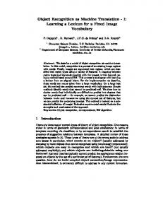

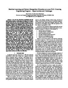


![[ePub] Download Pattern Recognition and Machine Learning ...](https://m.moam.info/img/260x300/epub-download-pattern-recognition-and-machine-lear_64786660097c474d228d1c27.jpg)
![Bishop: Pattern Recognition and Machine Learning [PDF]](https://m.moam.info/img/260x300/bishop-pattern-recognition-and-machine-learning-pd_647e06e9098a9ed70a8b45d4.jpg)

![[PDF] Download Pattern Recognition and Machine Learning ...](https://m.moam.info/img/260x300/pdf-download-pattern-recognition-and-machine-learn_64785ad5097c4796708cb7b3.jpg)
