IMPROVING SPEAKER VERIFICATION WITH FIGURE OF MERIT TRAINING Xiaohan Li*1, Eric Chang and Bei-qian Dai* Microsoft Research Asia *Department of Electronic Science and Technology, University of Science and Technology of China
[email protected],
[email protected]
A novel discriminative training method of Gaussian mixture model for text-independent speaker verification, Figure of Merit (FOM) training, is proposed in this paper. FOM training aims at maximizing the FOM of a ROC curve by adjusting the model parameters, rather than only approximating the underlying distribution of acoustic observations of each speaker that Maximum Likelihood Estimation does. The text-independent speaker verification experiments were conducted on the 1996 NIST Speaker Recognition Evaluation corpus. Compared with standard EM training method, FOM training provides significantly improved performance, e.g. the detection cost function (DCF) was reduced to 0.0286 from 0.0369 and to 0.0537 from 0.0826 in matched and mismatched conditions respectively.
metric used to evaluate the system such as the error rate directly. A speaker verification system can be evaluated using a metric called Figure of Merit (FOM). In this paper, we propose a novel discriminative training method of the speaker models for speaker verification task referred to as FOM training. The goal of FOM training is to maximize the FOM of a Receiver Operating Characteristic (ROC) curve and has previously been successfully used in wordspotting [5, 6]. The benefit of FOM training is that the system designer can easily change the definition of FOM to cover the region of interest in the ROC curve and devote more parameters of the speaker verification system to perform well in this region of interest. Detailed discussion will be included in Section 3. Evaluation experiments have been conducted to compare the performance of GMM's trained with different methods. It is shown that GMM's trained with this new method provide much improved discriminative ability compared to those trained with the ML criterion. The experimental results will be shown in Section 4. Lastly, Section 5 provides our conclusion.
1. INTRODUCTION
2. THE BASELINE SYSTEM
Security and authentication in speech-driven telephony applications can be achieved effectively through speaker verification (SV). Among the most successful approaches to robust textindependent speaker verification is the Gaussian Mixture Model (GMM) employed in many state-of-the-art systems [1, 3, 4]. For example, the system employing Bayesian adaptation of speaker models from a Universal Background Model (UBM) and handset-based score normalization (HNORM) has been the basis of the top performing systems in the past several NIST Speaker Recognition Evaluations [4]. The standard training approach of a hypothesized speaker model is based on Maximum Likelihood Estimation (MLE) which can be either dependent or independent of the UBM [3]. The ML criterion aims at modeling the underlying distribution of acoustic observations from the target speaker. In reality, the estimated distribution often deviates from the true distribution due to incorrect modeling assumptions and insufficient training data. Hence, the optimal ML criterion for density estimation does not imply an optimal classifier design. Some discriminative training methods have been proposed to improve the discriminative ability of the GMM's for either speaker identification [7, 9] or speaker verification [2]. It's natural to find a discriminative training method which optimizes the
For a GMM-UBM baseline system, a 2048-mixture UBM is trained on a large number of speakers (6 hours of speech from all the 43 male and 45 female speakers of the 1996 NIST Speaker Recognition Development corpus). For each target speaker, a 64-mixture GMM is trained with the Expectation-Maximization (EM) algorithm independently of the UBM. The score (or average log-likelihood ratio) of a given test segment O = {O1 ..., OT} is computed as:
ABSTRACT
score =
(1)
where T is the length of the test segment, Ot is the feature vector at time t and λtar and λUBM are parameters of the target model and UBM respectively.
3. FIGURE OF MERIT TRAINING The ROC curve is a plot of the false rejection rate versus the false acceptance rate of a SV system. One of its variant using a normal deviate scale for each axis, the Detection Error Tradeoff (DET) curve, has been widely used in representing a SV system's performance [1, 3, 4]. The closer the curve is to the axes, the better the performance of the SV system is.
1 This work was carried out during the first author’s internship at Microsoft Research Asia.
0-7803-7402-9/02/$17.00 ©2002 IEEE
1 T ∑ (log p(O t | λtar ) − log p(O t | λUBM )) T t =1
I - 693
The FOM is calculated by averaging the correct rejection rate (1 - false acceptance rate) of the system over a range of false rejection rates. The calculation of FOM is illustrated in Figure 1. In this paper, we average the correct rejection rate over the range of 0 to 50 percent of the false rejection rate. Hence, the FOM training attempts to train model parameters to maximize the FOM of a SV system. To adjust the model parameters, a gradient relating the FOM to each parameter is derived. Each trial's impact on the overall FOM is estimated by averaging the ratio of the change in overall FOM to that in the trial score as the score is varied over a small range. After the gradient has been calculated, parameters are adjusted in the direction that increases the FOM. The discriminative ability of the models is improved as trials from target (target trial) and impostor (impostor trial) are used to modify the parameters of the models.
3.1. Calculation of the FOM Gradient Since the FOM is calculated by sorting the scores of true and impostor trials separately for each target speaker and forming ROC curves, these measures and their derivatives can not be computed analytically. Instead, the FOM and its derivative are computed in the following way. Given enough target and impostor trials, a smooth ROC curve can be computed by sorting the target and impostor trial scores respectively. For each score in the sorted lists, the change of the FOM can be calculated by varying the score in a small range, hence the FOM gradient of this score can be calculated as:
grad (score) =
Change in FOM Change in score
(2)
50
DK
Probability of False Rejection (%)
45 40 35 30
Dk
25 20 15 10 5
FOM =
1 K
K
∑D
k
D1
k =1
0 0
5
10
15
20
25
30
35
40
45
50
Gradient
Target Gradient
Impostor Gradient
Trial Score
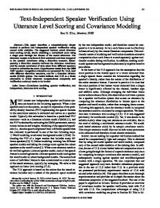
Figure 2: The FOM gradient versus the trial score for target and impostor speaker. The score range is calculated for the target and impostor trials respectively. Let grad (score) be the FOM gradient for the given score calculated by (1), it can be estimated by:
grad (score) =
1 L i ∑ grad score + M score _ range (4) 2L i = − L i≠0
where L is the number of samples which are used to average the estimated gradient by moving the given score forward or backward, score_range/M is the moving step size. L is 9 and M is 8 in this paper. Sufficient target and impostor trials are needed to compute a smooth ROC curve. We use vector groups as verification trials since there are only a limited number of training segments from each target speaker. A vector group is a series of consecutive vectors derived from the training sentence, and the index of the first vector of this group is randomly selected from the training segment. In this paper, the size of a vector group is 15, and the groups in the sorted target or impostor trial lists are both 1000. Figure 2 shows plots of linearly scaled FOM gradients versus target and impostor trial scores for one target speaker. Dots are target gradients, and circles are impostor gradients. This figure shows the impact of a target trial to the FOM as its score varies. When the score is very high, the target trial has no impact because it is ranked above all the impostor scores and thus has no change in FOM. As the score becomes lower, it is surpassed by more and more impostor scores. There are thus larger positive gradients for this score. The impostor trial gradients behave in the opposite direction of the target trial gradients.
Probability of False Acceptance (%)
3.2. Adjusting Model Parameters
Figure 1: Receiver Operator Characteristic (ROC) curve and the calculation of Figure of Merit. Because of the quantized nature of the change in FOM, the gradient estimate is averaged over a series of samples from a range around the given score. The score range is calculated by taking the difference between the scores of the 20th percentile trial and 80th percentile trial for the target speaker. Let score[n%] represent the score of the nth percentile trial. The score range is calculated with the formula:
score _ range = score[20%] − score[80%]
Our aim is to maximize the FOM of a SV system by adjusting the GMM parameters. We adopt a gradient descent scheme in FOM training. Let x(t) denote the parameter of a GMM at time t, then parameter at time t+1 is obtained by the formula: ∂FOM ∂x ∂FOM ∂score = x (t ) + η ⋅ ⋅ ∂score ∂x ∂score = x (t ) + η ⋅ grad ( score ) ⋅ ∂x
x (t + 1) = x (t ) + η ⋅
(3)
I - 694
(5)
In these experiments, we focus on the male target speakers using two-handset training condition (two minutes of training speech extracted from two sessions originating from different telephone handsets, one minute per session) and the 30 second test condition. This corpus consists of 21 male target speakers and 204 male impostors. There are 321 and 332 target trials in matched and mismatched conditions respectively, and 1060 same-sex impostor trials.
Target Training Data
EM Training
EM Trained Target Model
4.2. Front-end Processing Impostor Training Data
FOM Training
UBM
FOM Trained Target Model
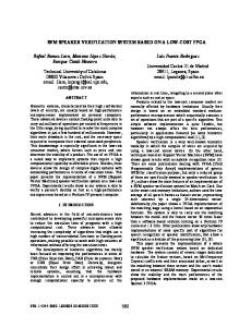
Figure 3: The training methodology for FOM training. where η is the learning rate. In this paper, only the mean values of the target GMM are adjusted:
mki (t + 1) = mki (t ) + η ⋅ grad (score ) ⋅
wk N (O; m k , σ k )
∑ w N (O; m J
j
j =1
j
,σ j )
⋅
Oi − mki (t ) (6)
σ ki
In this equation, J is the number of mixtures of a GMM, mki (t) is the ith component of the mean vector for the kth Gaussian mixture of the GMM at time t, σki is the standard deviation of the ith component for the kth Gaussian mixture, wk is the kth mixture weight, and O is one of the observation vectors in the vector group. η is initialized to be the reciprocal of the sum of the absolute values of gradients before the first iteration and is multiplied with a shrinking factor of 0.95 at each following iteration.
First, the speech is pre-emphasized with a factor of 0.97 and segmented into frames by a 32-ms Hamming window progressing at a 16-ms frame rate. Then 10 MFCCs except for the 0th component are extracted from the speech. Cepstral analysis is performed only on the passband (300-3400Hz) of the telephone speech. Finally, both RASTA filtering and Cepstral Mean Subtraction (CMS) are used to remove linear channel convolutional effects on the cepstral features.
4.3. Evaluation Results The SV performance is assessed using both the DET curve and a Detection Cost Function (DCF), which is defined by NIST as a weighted sum of the false acceptance and false rejection error probabilities as determined from a system's actual decisions [1]:
C Det = C fr ⋅ Pfr ⋅ PTar + C fa ⋅ Pfa ⋅ PImp
(7)
where Pfr and Pfa are the false rejection and false acceptance rates respectively. Other required parameters in this function are the cost of a false rejection (or missed detection, Cfr), the cost of a false acceptance (or false alarm, Cfa), the a priori probability of a target speaker (PTar) and the a priori probability of an impostor (PImp). The costs were set to Cfr =10 and Cfa =1 while the prior probabilities were PTar = 0.01 and PImp=0.99 [1].
3.3. Training Methodology Figure 3 describes the methodology used for applying FOM training. First of all, for each target speaker, the target model is trained by EM algorithm with the target speaker's training data. Then FOM training is applied to the target model to maximize the FOM by adjusting the mean values of all the mixtures with the gradient descent scheme. In each FOM training iteration the sorted target and impostor trial score lists are calculated with the randomly selected vector groups from the target and impostor training data against the target model and the UBM. Then the FOM gradient for each score is evaluated with (2) and (4), and finally the mean values of the model are adjusted by all the vectors in this vector group with (6). The FOM training procedure is stopped after 25 iterations when no apparent increase of the FOM on the training set can be observed.
Match Mismatch
Speaker verification experiments are carried on the 1996 NIST Speaker Recognition Evaluation corpus [8]. The available telephone numbers per conversation was exploited to create matched and mismatched telephone handset (or number) test conditions.
FOM 0.0286 0.0537
Rel. Reduction 22% 35%
Table 1: Minimal DCFs for models trained with EM algorithm and FOM training method in matched and mismatched conditions. The DET curves are shown in Figure 4. In the upper plot of Figure 4 we show results for the matched target telephone handset (or number) tests; in the lower plot of Figure 4 we show results for the mismatched target handset tests. The circles on the plots represent the operating points for which the DCF's are minimal. The minimal DCF's are shown in Table 1. It's clear from the results that FOM training significantly outperforms EM algorithm in both matched and mismatched conditions.
4. EXPERIMENTS 4.1. Evaluation Corpus
EM 0.0369 0.0826
5. CONCLUSION This paper has compared two approaches of training the target speaker model for a text-independent speaker verification task using GMM's. The 1996 NIST Speaker Recognition Evaluation corpus was used to conduct the experiments. It was shown in the experiments that the discriminative ability of GMM was
I - 695
improved with FOM training, and a system with target models further trained by FOM training produced superior performance compared with target models trained with only the EM algorithm, both in matched and mismatched conditions.
with target models adapted from the UBM with Bayesian adaptation has been the basis of the state-of-the-art systems. Our future work will focus on the incorporation of FOM training with the adaptation methods.
6. ACKNOWLEDGMENT The authors thank Jianlai Zhou, Chao Huang, Chengyuan Ma and other members of the speech group at Microsoft Research Asia for many fruitful discussions.
7. REFERENCES [1] A. Martin and M. Przybocki, “The NIST 1999 Speaker Recognition Evaluation – An Overview,” Digital Signal Processing, vol. 10, pp. 1-18, 2000.
EM FOM
[2] A. E. Rosenberg, O. Siohan, S. Parthasarathy, “Speaker Verification Using Minimum Verification Error Training,” Proc. of ICASSP’98, pp. 105-108, May 1998. [3] D. A. Reynolds, “Comparison of Background Normalization Methods for Text-independent Speaker Verification,” Proc. of EUROSPEECH’97, pp. 963-966, 1997. [4] D. A. Reynolds, T. F. Quatieri, and R. B. Dunn, “Speaker Verification Using Adapted Gaussian Mixture Models,” Digital Signal Processing, vol. 10, pp. 19-41, 2000. [5] E. I. Chang, “Improving Wordspotting Performance with Limited Training Data,” Ph.D. Thesis, Massachusetts Institute of Technology, 1995. [6] E. I. Chang and R. Lippmann, “High-Performance LowComplexity Wordspotting Using Neural Networks,” IEEE Trans. Signal Processing, Vol. 45, Issue: 11, Nov. 1997.
EM FOM
[7] J. He, L. Liu, and G. Palm, “A Discriminative training algorithm for Gaussian Mixture Speaker Models,” Proc. of EUROSPEECH'97, pp. 959-962, 1997. [8] NIST, “The 1996 Speaker Recognition Evaluation Plan,” http://www.nist.gov/speech/tests/spk/.
Figure 4: DET curves for models trained with EM algorithm and FOM training method in matched (upper) and mismatched (lower) conditions.
[9] O. Siohan, A. E. Rosenberg, S. Parthasarathy, “Speaker Identification Using Minimum Classification Error Training,” Proc. of ICASSP’98, pp. 109-102, May 1998.
FOM training was only applied to the EM trained target models independently of the UBM in this paper. The system
I - 696