Improving the Computation Efficiency of COBRA-TF for LWR ... - Ipen.br

PHYSOR 2004 -The Physics of Fuel Cycles and Advanced Nuclear Systems: Global Developments Chicago, Illinois, April 25-29, 2004, on CD-ROM, American Nuclear Society, Lagrange Park, IL. (2004)

Improving the Computation Efficiency of COBRA-TF for LWR Safety Analysis of Large Problems Diana Cuervo*1, Maria N. Avramova2 and Kostadin N. Ivanov2 1 Department of Nuclear Engineering, Polytechnic University of Madrid Avda. Arco de la Victoria s/n, 28040 Madrid, Spain 2 Department of Mechanical and Nuclear Engineering, The Pennsylvania State University 230 Reber Building, University Park, PA 16802, USA A matrix solver is implemented in COBRA-TF in order to improve the computation efficiency of both numerical solution methods existing in the code, the Gauss elimination and the Gauss-Seidel iterative technique. Both methods are used to solve the system of pressure linear equations and relay on the solution of large sparse matrices. The introduced solver accelerates the solution of these matrices in cases of large number of cells. The execution time is reduced in half as compared to the execution time without using matrix solver for the cases with large matrices. The achieved improvement and the planned future work in this direction are important for performing efficient LWR safety analyses of large problems. KEYWORDS: efficiency, subchannel analysis, numerical methods, matrix solver. 1. Introduction The increased use of detailed descriptions of reactor core for subchannel safety analysis is making necessary to improve code numerical method performance and speed in order to obtain reasonable running times for large problems. In the case of two-fluid codes due to the extended set of complex equations the necessity of a highly efficient numerical method and matrix solver is even more pronounced. COBRA-TF [1] is a two-fluid, three-field code (continuous vapor, continuous liquid and entrained liquid drops) for two-phase flow problems. The three field conservation equations for multidimensional flow are discretized using semi-implicit finite-difference technique with donor cell differencing for the convected quantities. The formed in this way set of algebraic equations must be solved simultaneously over each cell as well as for the entire computational mesh in order to obtain parameter distributions for the different fields. One of the most important steps in the solution process in terms of CPU time is the solution of a system of linear equations that relate pressure in each node of the computational mesh. Since the dimension of the matrix of this system is usually large the use of an optimized matrix solver could reduce the duration of the solution process significantly. The purpose of this work was to investigate the application of a new optimized matrix solver to the analysis of large problems using both the direct inversion and Gauss-Seidel iterative methods for the solution of the system of pressure equations.

*

Corresponding author, Tel. + 34-91-336-7177, FAX +34-91-544-2149, E-mail: [email protected]. Visiting scholar at Department of Mechanical and Nuclear Engineering, The Pennsylvania State University

2. Numerical solution of the two-fluid equations in COBRA-TF The two-fluid three-field semi-implicit finite difference equations must be simplified to be solved in a reasonable amount of time although they must converge to the correct solution. 2.1 Solution scheme of the two-fluid equations The first stage in the solution process (outer iteration), performed at every time step, is to solve the momentum equations using currently known values for all the variables to obtain an estimate of the new time step flow for every cell. All explicit terms in the momentum equations are computed in this stage and are assumed to remain constant during the remainder of the time step. Tentative velocities can be now calculated in order to be introduced in the continuity and energy equations. As second stage the block Newton-Raphson method is used to obtain the variation of each independent variable required to bring the residual errors to zero. The residual errors (ECL, EEV, EEL, ECE, ECV and ECG) appear when the new velocities are used to compute the convective terms in these equations. As example of equation residual form we show vapor mass equation for channel i and section j: ECV

[(α ρ ) − (α ρ ) ]A = n v v j

v v j

∆t

cj

NA

+∑

KA=1

[(α ρ )*U~ A ] v v

vj

m j KA

∆xj

NB

−∑

[(α ρ )*U~ v v

]

Amj−1 KB

v j−1

∆xj

KB=1

NKK ~ ] − Γj − Scvj − ∑SL[(αvρv ) *V vL j ∆xj ∆xj L=1

(1)

where * symbol means donor cell quantities, n superscript means quantities at new time step and ~ symbol over the velocities U indicates that they are the tentative values computed from the momentum equations. ρv and αv are the density and void fraction of vapor, Ac and Am are the continuity and momentum cell cross section areas, Γ is the net rate of vapor generation, NKK number of transverse connections, NA and NB number of connections to top and bottom of cell, V transverse velocity and Scv net entrainment rate of vapor. The system should be linearized with respect to the independent variables αv, αvhv, (1-αv)hl, αe and pressure of the actual cell and those in contact with it, i.e, Pj, Pi with i=1,NCON, where NCON is the number of cells in contact with the one of interest. Applying the Newton-Raphson method one can obtain the matrix equation (2) for each cell.  ∂E CG  ∂α g   ∂E CL  ∂α g  E ∂ CV   ∂α g   ∂E CE  ∂α g  ∂E  EL  ∂α g  ∂E  EV  ∂α g

∂E CG ∂α v ∂E CL ∂α v ∂E CV ∂α v ∂E CE ∂α v ∂E EL ∂α v ∂E CG ∂α v

∂E CG ∂α v h v ∂E CL ∂α v h v ∂E CV ∂α v h v ∂E CE ∂α v h v ∂E EL ∂α v h v ∂E EV ∂α v h v

∂E CG ∂ (1 − α v )h l ∂E CL ∂ (1 − α v )h l ∂E CV ∂ (1 − α v )h l ∂E CE ∂ (1 − α v )h l ∂E EL ∂ (1 − α v )h l ∂E EV ∂ (1 − α v )h l

∂E CG ∂α e ∂E CL ∂α e ∂E CV ∂α e ∂E CE ∂α e ∂E EL ∂α e ∂E EV ∂α e

∂E CG ∂Pj ∂E CV ∂Pj ∂E CV ∂Pj ∂E CE ∂Pj ∂E EL ∂Pj ∂E EV ∂Pj

∂E CG ∂Pi =1 ∂E CV ∂Pi =1 ∂E CV ∂Pi =1 ∂E CE ∂Pi =1 ∂E EL ∂Pi =1 ∂E EV ∂Pi =1

L L L L L L

∂E CG  ∂PNCON   δα g    ∂E CV   δα v    E CG  ∂PNCON  δα h   v v E  ∂E CV     CL  ( 1 ) h δ − α v l E CV  ∂PNCON    = −  ⋅  δα e   ∂E CE   E CE    P δ j ∂PNCON    E EL    P δ     i = 1 ∂E EL E EV     M ∂PNCON    ∂E EV   δPi = NCON   ∂PNCON 

(2) This equation can be written in an operator form:

[R(x)]{δ(x)} = −E

(3)

where [R(x)] is the Jacobian of the system of equations evaluated for the set of independent variables (x) and composed of analytical derivatives of each equation with respect to linear variation of independent variables, δ is the solution vector containing these linear variations and E is the errors’ vector. After calculation of terms, the former system is analytically reduced using the Gaussian elimination to obtain solutions for the independent variables. Void fraction related variables and pressure for the actual cell are dependent on the pressure of adjacent cells (Equation 4).

r11 0  0  0 0   0

r12

r13

r14

r15

r16

r17

r22 0

r23 r33

r24 r34

r25 r35

r26 r36

r27 L r37 L

0

0

r44

r45

r46

r47 L

0 0

0 0

0 0

r55 0

r56 r66

r57 r67

L

L L

 δα g   δα  v  r1( 6+ NCON )    a1   δα v hv   a  r2 ( 6+ NCON )     2 δ (1 − α v )hl  r3( 6 + NCON )   a3    ⋅  δα e  = −  r4 ( 6+ NCON )    a 4  δPj    a5  r5( 6 + NCON )   δPi =1    r6 ( 6+ NCON )   a6   M    δPi = NCON 

(4)

After reducing the system an equation of the form:

δPj = a +

NCON

∑ g δP i =1

i

i

(5)

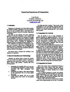
is derived for each cell. Thus a system with a number of equations equal to the number of computational cells should be solved in order to obtain the pressure variation for every cell. After this step the linear variation in the other independent variables is unfolded. A flow diagram of the process is shown in Figure 1. 2.2 Solution of the matrix of pressure system

In regard to the pressure equation, the size of this system depends on the number of cells in the problem. The dimension of the matrix is the square of the number of cells. For a case with a small number of cells the equation set may be solved by direct inversion. For a case with a large number of mesh cells a Gauss-Seidel iterative technique is recommended. This technique is based on splitting the mesh cells in groups of cells that influence greatly each other. These groups of cells are called simultaneous solution groups. Equation set is split in the same way. When a solution group is being solved the values of δPj for the cells that do not belong to the group are set to the previously calculated values. The multiplication of the pressure matrix by the independent variables’ vector produces a linear system with the same number of equations as the number of cells in the solution group. This system is solved by the Gaussian elimination. A Gauss-Seidel iteration (inner iteration) is carried out over the groups of cells to obtain the new pressure vector. Convergence is reached when the change in δPj for each cell from one iteration to the next fulfills a convergence criteria. The process is shown in Figure 2.

IN Solution of momentum eqns Mass, energy eqns linearization Newton-Raphson system reduction Solution of system pressure matrix Y

Outer iteration

Direct? N

Gauss elimination

Inner iteration

Perform one iteration step in Gauss-Seidel

δP converged?

Time step halved

N

Y Unfolding of indep. and dependent variables

Time step control

N

Y Proceed to next time step

Fig.1 COBRA-TF solution flow diagram.

δP1

Solution group 1

0

.

δPNSOL1

Solution group 2

≠0 0

Gauss-Seidel iteration

b1

. . .

. . .

δPNCELLS

=

Gaussian elimination

. . bNCELLS

Values from previous iterations Fig. 2. Gauss-Seidel iteration for the simultaneous solution groups.

As it was shown, in both numerical methods, currently implemented in the code, one or more linear equation systems must be solved by Gaussian elimination. It is obvious that the performance of this part of the solution process will influence greatly the code computation efficiency. 3. Library for efficiency improvement of direct inversion of matrices

COBRA-TF is using the Gaussian elimination to solve the system pressure matrix in both solution alternatives existing in the code. In order to improve the solution process performance some subroutines from SuperLU library were utilized. 3.1 SuperLU library SuperLU [2] is a general purpose library for the direct solution of large sparse systems of linear equations on high performance machines. The library is written in C and is callable from either C or Fortran. The library routines will perform a LU decomposition with partial pivoting and solution of the triangular system through forward and backward substitution. Three libraries exist - sequential, multithreaded, and distributed, and all of them use variations of the LU decomposition optimized to take advantage of both the sparsity and the computer architecture [3]. Sequential SuperLU was selected as the most adequate for our use. The library provides a large set of subroutines to perform different steps of LU decomposition as well as other tasks like performance statistics or error bounds computing. Two standard driver algorithms are included but the user should design an optimized one for the problem being solved. All subroutines are available in single and double precision and for real and complex input data. SuperLU depends on having a high performance BLAS (Basic Linear Algebra Subroutine) in order to be able to show high performance characteristics. In case this library is not available, SuperLU includes a default BLAS library with necessary subroutines. It is important to note that this library is not optimized for all machine architectures. The above mentioned subroutines have to be compiled with C compiler. In order to embed them in a Fortran program, bridge subroutines (as well in C language) have to be coded. The system matrix has to be stored in the Harwell-Boeing sparse matrix format, i.e. compressed column storage. 3.2 Library implementation in COBRA-TF Two new subroutines were developed as part of the matrix solver implementation. The first one, coded in Fortran, performs the transformation of the matrix of pressure into a Harwell Boeing format matrix in order to apply SuperLU subroutines to solve the system. Originally COBRA-TF only stores

the diagonal band of the matrix of pressure to save memory space due to the rest of matrix elements are zero. Thus this subroutine must carry out two tasks, recovering of the complete matrix of pressure and storage of this matrix in the Harwell-Boeing format. These two tasks must be done in only one step in order to save time in the solution process. The second subroutine, coded in C, performs the solution procedure steps to obtain the solution array for the system. In the factorization process two matrices, the column permutation matrix and the row permutation matrix (Pr A Pc=LU), must be calculated. These matrices do not change if the matrix A has the same sparsity structure and similar numerical entries for every time step as it is the case in subchannel analysis. Thus the first stage consists in the calculation of the permutation matrices if the code is solving for the first time step. After that, the code performs the calculation of L and U matrices at each time step and solution of the system through forward and backward substitution. The permutation matrices are stored to be reused at every time step. Memory allocation for L and U matrices is performed only at the first time step. This approach is designed not only to use an optimized matrix solver with better performance than the one implemented originally in the code, but as well to avoid unnecessary steps that need to be carried out only once. It was observed that the number of Gauss-Seidel iterations is strongly dependent on the time step size. At this moment COBRA-TF selects time step size to fulfill finite-difference equations convergence criteria. However, this time step selection algorithm can be optimized to improve inner iteration convergence. 4. Application of COBRA-TF with the implemented matrix solver

Two cases have been calculated to test the implementation performance. These calculations were carried out on a Pentium 4 machine with 1.2 GHz processor and 512 MB RAM. The first one is a flow reduction transient hot subchannel analysis of PWR (157 17x17 fuel assemblies). An embedded mesh [4] was used for this analysis. The interior channels are real thermalhydraulic channels within the assembly. From interior to exterior different size lumped channels were modeled until reaching a quarter of assembly size (Figure 3). The model contains 233 channels and 34 axial nodes per channel that means a matrix dimension of 7920×7920. Boundary conditions are inlet flow and enthalpy and outlet pressure. Axial and radial power distributions are obtained from 3D

Fig. 3. Embedded mesh configuration for subchannel analysis problem.

neutronic analysis. The calculation was performed using both methods, direct and iterative. For the iterative method, 34 simultaneous solution groups were selected for the calculation - one group per axial level. The results are shown in Table 1. The number of inner iterations in this case was up to 4. In the second case a PWR (157 17x17 fuel assemblies - FA) main steam line break (MSLB) scenario was simulated [5]. The inlet mass flow rate and enthalpy as inlet boundary condition at the core bottom and the system pressure as boundary condition at the top of the core are applied. The number of channels is 157 (one channel per FA) with 40 axial nodes per channel, which constitutes a pressure matrix of dimension 6280×6280. Both methods were again applied using 40 simultaneous groups for the iterative method. Due to the high number of iterations observed in this case that reduces in great manner the efficiency of the code a second calculation with time step optimization was performed. In this last case the optimization was carried out in a tentative manner without selection algorithm to reduce the inner iteration number up to 7 in most of the time steps. The CPU time results are shown in Table 1. Table 1 CPU time results Subchannel analysis Direct solution Gauss-Seidel iteration

Matrix solver implemented 6h 03min 2h 36min

Standard code 13h 25min 5h 24min

MSLB scenario Direct solution Gauss-Seidel iteration

Matrix solver implemented 3h 24min 3h 16min

Standard code 7h 19min 3h 12min

To prove that the matrix solver implementation do not introduce deviations to the COBRA-TF results two variables have been selected for analysis: pressure drop and phasic velocities. Table 2 shows the obtained axial distributions for a selected channel in the subchannel analysis case. It can be observed that the deviations are negligible in all comparisons. Similar situation with even smaller deviations is found in the MSLB scenario calculations. 5. Conclusions

One can see from the results presented in Table 1 that the new matrix solver implementation demonstrates a capability to reduce CPU times to half of the standard CPU times (without using the matrix solver) for both steady state and transient cases if the pressure matrices that must be solved are large enough to reach the size of matrix solver optimum performance. The use of the Gauss-Seidel iterative method reduces the dimension of matrices that must be solved by direct inversion to the square of number of simultaneous groups times the dimension of complete matrix of pressure system. Thus the dimension of these smaller matrices can be situated bellow the solver optimum performance limit. As conclusion it seems obvious that the larger the case is that must be solved the greater would be the reduction in CPU time compared to the standard CPU time. The combination of the Gauss-Seidel iterative method with the implemented matrix solver could allow analyzing much larger cases with the same CPU time.

Table 2 Deviations (in %) of selected predicted variables from values obtained from original methods for flow reduction transient hot subchannel analysis case.

Axial location (ft)

Press. Drop (psia)

12 11.8 11.61 11.41 11.21 11.04 10.89 10.52 10.07 9.62 9.18 8.8 8.36 7.91 7.47 7.09 6.64 6.2 5.75 5.38 4.93 4.49 4.04 3.67 3.22 2.77 2.33 1.95 1.64 1.33 1.02 0.72 0.42 0.19

0.03 0.04 0.04 0.03 0.04 0.03 0.03 0.04 0.03 0.03 0.03 0.02 0.02 0.02 0.02 0.02 0.01 0 0.01 0.01 0 0 0 0 0 0 -0.04 -0.05 0 0 0 0 -0.09 0.03

Gauss Seidel (a) Liquid Vapor Velocity Velocity (ft/s) (ft/s)

0 0.06 0.06 0 -0.06 -0.06 0 0.06 0.06 0.07 0 0 0 0 0 0 0 0 0 0 0 0 0 0.08 0 0 0 0 -0.08 -0.08 0 -0.08 -0.08 0

-0.05 0 -0.11 0.17 0.45 -0.17 0 0.06 0.17 0.30 -0.18 0.25 -0.31 -0.21 0.07 0.07 0.07 0 0 0 0 0 0 0 0 -0.08 0 0.40 0.08 -0.33 0.25 0 -0.08 0.41

Matrix solver imp. (b) Press. Liquid Vapor Drop Velocity Velocity (psia) (ft/s) (ft/s)

0.04 0.04 0.04 0.04 0.04 0.04 0.03 0.04 0.03 0.03 0.04 0.03 0.03 0.03 0.03 0.03 0.03 0.02 0.03 0.03 0.02 0.02 0.04 0.05 0.02 0.03 0 0 0.05 0.06 0.07 0.08 0 0.04

0 0.06 0.12 0.12 0 -0.06 0 0.06 0.06 0.07 0 0 0 0.07 0 0.07 0.07 0.07 0 0 0 0 0 0.08 0 0.08 0 0.08 -0.08 -0.08 0 0 0 0.08

-0.05 -0.27 0.27 0.55 0 -0.33 -0.15 -0.06 0.17 0.18 0.18 0.13 -0.31 0.20 0.07 0.07 0.15 0.07 0 0 0 0 0 0 0 -0.72 -0.49 0.24 0.57 0.08 0.16 -0.33 -0.67 0

Matrix solver imp. in G.S. (c) Press. Liquid Vapor Drop Velocity Velocity (psia) (ft/s) (ft/s)

0.02 0.02 0.02 0.03 0.03 0.03 0.02 0.02 0.02 0.02 0.02 0.02 0.02 0.03 0.02 0.02 0.02 0.02 0.01 0.01 0.03 0.02 0.02 0.02 0.02 0.03 0.04 0.09 0.05 0.06 0 0.08 0.09 0.02

0.12 0.06 0 0.06 0.06 0.06 0 0 -0.06 -0.07 0.07 0.07 0.07 0.07 0.07 0.07 0 0.07 0 0.08 0 0 0 0 0 0 0 0 0 0.08 0 0.16 0.08 0.08

0.38 0.22 0.06 0.22 -0.22 0.22 -0.05 0 -0.11 -0.18 0.35 -0.13 0.37 0.21 0.07 0 0 0.07 0 0.07 0 0 0.08 0 0.08 -0.16 -0.49 -0.24 -0.08 0.08 0.41 -0.08 -0.50 -0.08

(a) Deviation of results using Gauss-Seidel iterative method from values obtained by direct solution using Gauss elimination. (b) Deviation of results using the direct solution with matrix solver implemented from values obtained by direct solution using Gauss elimination. (c) Deviation of results using the Gauss-Seidel iterative method with matrix solver implemented from values obtained using Gauss-Seidel iterative method. Another important conclusion of the study carried out for this work is that the efficiency of the method used by the code to solve the set of system pressure linear equations will affect the code efficiency in a great manner. So far the code is using either Gauss elimination or a Gauss-Seidel iterative technique. During last years, considerable research has been performed in a class of techniques known as Krylov subspace methods or non-stationary iterative methods which include the classical conjugate gradient method. The superior performance of

Krylov solvers as compared to the stationary iterative methods (to which Gauss-Seidel method belongs) has been well documented for the few-group neutron diffusion equation solution [6] as well as for phasic continuity equation solution in VIPRE-02 [7], which is a two-fluid two-field code for subchannel analysis. The implementation of a non-stationary method for the solution of the matrix of pressure system in COBRA-TF would increase further the efficiency of the code and this is the subject of planned future work in this direction. The use of the matrix solver, implemented during this work, in the solution of linear systems that must be solved in most of the Krylov subspaces methods with the preconditioner matrix could represent an additional increase in the method efficiency that will be studied. Acknowledgements The authors wish to thank SuperLU library developers, James W. Demmel, John R. Gilbert and Xiaoye S. Li, for the work accomplished and freely distribution of the library. References 1) C.Y. Paik et al., “Analysis of FLECHT-SEASET 163-Rod Blocked Bundle Data Using 2) 3) 4)

5) 6)

7)

COBRA-TF”, NUREG/CR-4166 (1985). J.W. Demmel, J.R. Gilbert, S.L. Xiaoye, “SuperLU User’s Guide”, pp. 25-30 (2003). J.W. Demmel et al., “A Supernodal Approach to Sparse Partial Pivoting”, SIAM J. Matrix Anal. Appl. , 20 (3),pp. 720-755 (1999). J.M. Aragones, C. Ahnert, O. Cabellos, “Methods and Performance of the Three-Dimensional Pressurized Water Reactor Core Dynamics SIMTRAN On-Line Code”, Nuclear Science and Engineering, 124, pp. 111-124 (1996) K. Ivanov et al, “A PWR MSLB Benchmark, Final Specifications”, NEA/NSC/DOC(97)15, OECD Nuclear Energy Agency, (1997) H. Joo, T. Downar, “An Incomplete Domain Decomposition Preconditioning Method for Nonlinear Nodal Kinetics Calculating”, Nuclear Science and Engineering, 123, pp. 403-414 (1996) T. Downar, H. Joo, “A Preconditioned Krylov Method for Solution of the Multi-dimensional, Two-fluid Hydrodinamics Equations”, Annals of Nuclear Energy, 28, pp. 1251-1267 (2001)