Improving the efficiency of constraint logic programming languages by

Improving the efficiency of constraint logic programming languages by deriving specialized versions* M. Bruynooghe, V. Dumortier and O. Janssens** Department of Computer Science, K.U.Leuven Celestijnenlaan 200A, ]3-3001 Heverlee

Abstract

Extending logic programming to constraint logic programming has substantially broadened the range of problems solvable in a declarative style. However experiments with the Prolog Ill system showed that the generality of the constraint solving often incurs a h e a v y performance penalty for the - often occurring - special cases in which the problem has a simple algorithmic solution. This paper investigates - in the context of Prolog llI - the feasibility of automatically extracting specialized versions. This is illustrated on some examples. Extraction of the specialized version is based on a transformation technique "compiling control" which was originally devised for transforming logic programs requiring a special computation rule into Prolog programs.

1. I n t r o d u c t i o n Typical for logic programs is that, at least in principle, a predicate can be queried in different ways. So, generated code has to be general enough to cope with different kinds of data flow. The price to be paid for this generality is a performance penalty. The most important step in closing the performance gap with imperative languages has been the design of the W A M [10], but, for some programs, a substantial difference remains. To f u r t h e r close the gap, some authors have proposed to generate different versions - corresponding to different patterns of usage - for the same predicate [1, 8, 11], e.g. one version of append for concatenating and another for splitting lists. The introduction of constraint logic programming [3, 9] has broadened the range of problems solvable in a declarative style, but ff general constraint solving is always applied it also aggravates the performance gap. For a problem having a clean expression in Prolog, the difference in efficiency between its Prolog KI [4] program and its Prolog version running on a finetuned implementation can be substantial. Again, a w a y out *

Work accomplished with support from ESPRIT project PRINCE (CEC), National Funds fo~ Scientific Research (Belgium), DPW-B project RFO-AI-O2 (Belgium) ** Email: {maurice, veroniek, gerda}e cs.kuleuven.ac.be

310

seems to be to generate different versions for the same procedure and to select preferably at compile time - the appropriate version. Such a course has also been t a k e n b y Alan Borning in his constraint solving w o r k [6]. In this paper the problems associated w i t h automatic generation of specialized versions are studied f o r some Prolog III programs. The extraction of a specialized version is based on a t r a n s f o r m a t i o n technique "compiling control" [2, 5] which we have developed to t r a n s f o r m logic programs requiring a special computation rule into Prolog programs.

2. Examples In this section we consider some Prolog III programs together w i t h a description of the class of intended queries - given b y their instantiation pattern. For each a r g u m e n t one of the following abstractions is given : X [ denotes a free variable, X,g a ground term, X~ a n y t e r m and f(X1 . . . . . Xn) a t e r m w i t h f / n as functor w i t h Xi as abstraction of its ith argument. For each program and each instantiation pattern f o r the query, there exists an optimal or target program, which avoids the invocation of the general constraint solving techniques as m u c h as possible or, in other words, which is as close to ordinary Prolog as possible. For example, in case of numerical constraints, simple arithmetic evaluation and assignment m a y suffice, thus completely eliminating the use of the constraint solver. During the execution of a Prolog III program constraints are stepwise added to the set of constraints and t h e y are dealt w i t h by the corresponding constraint solver, w h i c h is considered as a black box. However, compile-time anaiysis can often reveal w h e n a particular constraint will be activated and h o w the dataflow inside it will be. In such cases, it is preferable to avoid activation of the general constraint solver. Instead, an ordinary Prolog call can be inserted at the appropriate place and directly be executed when activated b y the standard left to right computation rule. I n the sequel, such a compile-time anatysis is performed b y constructing and analysing a so called symbolic trace; the specialised version is then obtained b y synthesizing either a Prolog III or o r d i n a r y Prolog program f r o m the trace. The symbolic trace is basically an abstraction of an incomplete SLD-tree. Abstraction in the sense t h a t concrete arguments are replaeed b y their abstractions as explained above. The idea is explained in [2] and f o r m a l l y developed in [5]. The extension t o w a r d s CLP means t h a t a node (state) not o n l y consists of a conjunction of abstracted subgoals but atso of a conjunction of abstracted constraints (the latter enclosed b y { }). The computation rule is defined as follows: --Selection of a constraint has priority over the selection of an ordinary subgoal. However, a constraint m a y o n l y be selected as soon as it has become sufficiently instantiated. E.g., the numerical constraint X > Y is selected if the values of X and Y are known; the constraint X = Y -- Z is selected as soon as the value of at least t w o variables is k n o w n and it is then t r a n s f o r m e d into the appropriate call of is/2. - - I f no constraint is sufficiently instantiated, the l e f t m o s t ordinary subgoal is selected. - - I f no subgoals are left and the constraint set is not e m p t y , the constraint set has to be dealt w i t h b y the general constraint solving algorithm of Prolog HI.

311

2.1 E X A M P L E : L e n g t h o f a l i s t

Original program* length([], 0). length([H I T], N):- length(T, NT) { N > 0, N T = N - 1 }. We consider t w o classes of queries w i t h the following instanttation patterns : length(LV,N g) to construct a list of variables of a given length and length(Lg,N v) to compute the length of a given list. Note that the first class can easily be generalized to length(La,N g) in order to include length(Lg,Ng). For each class of queries we first give the target program and then we investigate the transformation process.

2.1.1 length(LV,N e) Target program In this case general numerical constraint solving, which calls upon the simplex method, can be completely eliminated : the aimed specialization has a clean expression in Prolog: length([], 0). length([H I T], N):- N > 0, N T is N - 1, length(T, NT).

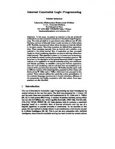
Symbolic trace The construction of the symbolic trace tree is illustrated in Fig. 1. ! State 1 shows the abstraction of the SI: length(LlV,N~g) { } query, i.e. the goal length(L~,Ng~). L1v = [l ~ L1v = [H2V[T2v] NlS = ~ / Using the first clause, the " ' 2 un~ficatlons L I" = [] and N~ = 0 are [] {} S2tengih(T2V,NT2 v) {NIl > 0, NT2v = NIg- 1 } performed. The first one causes L1 t to become ground. The arc of the 3 $3:length(T2V,NT2v) { NT2v = N]g - 1 } trace tree is labelled with these unifications. The derived state is the e m p t y goal O. Use of the second dVT2~) I } clause causes a unification L~ = [H~[T~] and yields the state labelled $2. In this state, the Fig. 1: Symbolic trace tree of length(LV,Ng). The selected subgoal or constraint is printed in italic constraint N~ > 0 is selected and state $3 is derived.

I

Now, the constraint NT~ = N~ -- 1 is selected. Its activation instantiates NT~, making it ground (NT~) in the next state. This state is actually a renaming of the starting state. It is useless to continue (the trace tree could be folded into a graph) since one would o n l y repeat the same pattern.

*

We do n o t use the original Px~log HI s y n t a x but the m o r e f a m i l i a r Edinburgh variant; typical f o r Prolog HI are the constraints enclosed by { }.

312

Synthesis The key is to replace the constraints by appropriate subgoals, i.e. the constraint N~ > 0 b y the subgoal N~ > 0 and NT~ = N~ - 1 by NT~ is N~ -- 1. One can then apply the synthesis technique described in [2] and [5]. This yields the following (meta)program: Sl(length([],0)). Sl(length([H I T],N)):- N > 0, NT is N - 1, Sl(length(T,NT)). Applying a simple transformation - eliminating the superfluous f u n c t o r s as described in [7] - w o u l d yield a renaming of the target program.

2.1.2 length(Lg,N ~) Target program Again, we w a n t to obtain an ordinary Prolog program in which general numeric constraint solving is no longer performed.

length([], 0). length([H I T], N):- length(T, NT), N is NT + 1/*, N > 0 */. Note that the test N > 0 will automatically be fulfilled. However, elimination of redundant constraints is not straightforward; its discussion, as well as the derivation of a version w i t h accumulating parameters, is beyond the scope of thin paper.

Symbolic trace

1 P: length(Llg,N1v) 1}

L1g = [l-12vlT2v]

-

2 p: length(T2g,NT2v) {NIV>0, NT2V=NI v- I }

[] {}

NT2v = 0

~

T2g _--[113v [T3 v]

3 Q: [] { NI v > 0, NT2g= NIv - 1 }

5 P: length(Tfl,NT3v) { ( NT2 v > 0, NT3 v= NT2 v - 1 ),

4

[] {N1g>O }

(NlV > 0' NT2V=NlV" 1 ) } NT3v = 0 T3g =[] /

6 Q: { ( NT2v > 0, NT..,g=N/'2" - 1 ), [] 1}

(1,,1:'1>o, rcr2" =N{'- 1 ) } 7 { (NT2g > 0), (NIY > 0,NT2g=NIv- 1 ) }

I 8

Q:{ ( NIV >O, NT2g = N1V-1 ) }

I

9

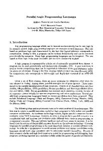
{(N:>O)} I o{} Fig. 2: Symbolic trace tree of length(Lg,N v)

10

313

The symbolic trace tree constructed for the abstract call pattern length(L~,N~) is shown in Fig. 2. The numerical constraints are delayed until they are of the form N~ > 0 and NT~$+t = N[ - 1 respectively. States 1, 2, 5 and 10 are all states having one goal length(T~,NT v) and zero or more times the group of constraints { bIT[ > 0, NTv+I = NT v -- 1 }. Such states, although not renamings of each other, are easily recognized in an automatic way [5] Consequently, is is not necessary to construct the symbolic trace beyond state 10.

Synthesis Again, the basis of the synthesis is to replace constraints by ordinary subgoals, i.e. the constraint NT~ > 0 by the subgoal NT~ > 0 and the constraint NT~+I = NT[ -- 1 by NT[ is NT~+1 + 1. Applying the synthesis of [2, 5] yields the following program: I(length(L,N)):- P(length(L,N), []). /* P - Q transitions */ V(length([],0), Cs):- Q(Cs). /* P - P transitions */ V(length([HIT],N), Cs):- V(length(T,NT), [N>0, NT--N-1 I Cs]). /* Q - [2 transitions */ Q([]). I* Q - Q transitions *I Q([N > 0, NT = N - 1 I Cs]):- N is NT + 1, N > 0, Q(Cs). This program is tatl-recursive but has the drawback that the list of constraints to be processed is carried around (the operations to be performed after completing the recursive predicate P are stacked). A slight improvement could be to stack only the variables NTi; the constraints can then be reconstructed within the Q predicate. However, a more important optimization turns up when analyzing the symbolic trace: instead of recursively activating constraints within the Q predicate, they can be shifted back to their original context (where they were created). In fact, this corresponds to replacing the constraints in the original program by ordinary subgoals and by then simply reordering these goals. The second clause is then rewritten as length([HIT],N):length(T, NT), N is NT + 1, N > 0 . This corresponds exactIy to the target program.

2.1.3 Discussion In these two examples, we notice that constraints are generated, selected and executed according to a very regular pattern. This allows to replace them by ordinary subgoals and to insert these at the right place to be activated by the standard computation rule of Prolog. In general, the synthesized program explicitly manipulates the constraint set. Often however - as in both cases above - the explicit storage and selection of constraints can be eliminated, when constraints can be activated within their original scope; tht.r corresponds to finding an adequate ordering of the subgoals. We expect that these observations hold for many simple predicates. We envision it is worthwhile to consider the development of libraries of specialized versions of such basic predicates. When used in conventional ways (to be detected at compile-tlme when possible) a very fast version (in fact faster than in nowadays commercial Prolog

314

systems as more information, i.e. mode information, is available) should be selected; when used in irregular ways, the general purpose Prolog III version can be selected. 2.2 EXAMPLE: P e r m u t a t i o n s o r t o f a P r o l o g HI l i s t

Original program sort(L, S) :-ord(S), perm(L,S) { L :: N , S :: N}. perm(,). perm(.Y, < U > . V ) :- del( U, .Y, W), perm(W, V). del(X, < X > . Y , Y). del(X, < Y > . U , .V):-del(X,U,V).

ord(). ord(.). ord( .T):- o r d ( < Y > . T ) { X = < V }. This Prolog HI program deviates from ordinary Prolog programs in two respects. Firstly, instead of ordinary Prolog lists, It uses so called tuples [4]. < > denotes the empty tuple, with n > 0 denotes an n-element tuple a n d . denotes tuple concatenation. Secondly, the constraint X :: N denotes that X is a N-element tuple. The program has a typical Prolog I~ style : first, the whole system of ~ constraints is created; next, perm is executed and a ~ constraint is activated as soon as possible and

forces backtracking in case of failure.

Target program (for the pattern sort(Lg,S~)) sort(L,S):compute length(L,N), construct_tuple(S,N), permord(L,S). permord(< > , < > ). permord( < X > .Y, < U > . V ) :delete(U, < X > . Y , W), po(W,U,V).

po(,~ 3. po(.Y, Uprev, < U > . V ) :delete(U, .Y, W), Uprev --< U, po(W,U,V). The generation of the output list by perm and the generation of the tests by ord are synchronized in such a way that the ~ constraint can be executed as a testing subgoal. Due to the special internal representation of tuples, it is desirable to have the subgoals corntmte_~ngth(L,N), computing the length of tuple L, and construct_.tuple(S,N), constructing a tuple of length N, although they are strictly speaking redundant.

Symbolic trace The symbolic trace is developed in Fig. 3. First, the constraint L~ :: N[ is selected. It translates Into the subgoal computeJength(Lgl,N~l); its effect Is to bind N[. Next, the constraint S[ :: N~ is selected; it translates into the subgoal construct_tuple(~,N~) and v ~r the effect is to create an n-place tuple which is abstracted as < E t .....En> (n>~0). Then, ord() is selected. This results in creating the set of constraints {

315

E~
), perm(Lig,) { }

I details omitted 5 R: perm(Llg,) { ElY =< E2V..... En.lV =< EnV } Llg =

Llg = .Y2v

= / []

~

= .V2v 6

del(El~,.r2g,w2v), perm(W2V,) { E 1v =< Ezv, .... E..I v =< F~v } I details omitted 7 S: perm(W2g,) { Elg =< E2v..... N . I v =< Env }

W2' = / = o

D

~

W2g= *:X3V>'y3v 8

= .V3v

del(E 2V,.Y3g,w3v), perm(W3V,) { Elg =< E2v..... ]~n_lv =< l~.nV }

9

details omitted

perm(W3g,) [ Elg =< Eft, E2g =< E3v, .... En_lv =< Env }

I

10

S:perm(W3g,