idea including 1 the soft-assignment of patches to visual words [2,3] or the use .... kernel classifier using the kernel (2) is equivalent to learning a linear classifier.
Improving the Fisher Kernel for Large-Scale Image Classification Florent Perronnin, Jorge S´ anchez and Thomas Mensink Xerox Research Centre Europe (XRCE)
Abstract. The Fisher kernel (FK) is a generic framework which combines the benefits of generative and discriminative approaches. In the context of image classification the FK was shown to extend the popular bag-of-visual-words (BOV) by going beyond count statistics. However, in practice, this enriched representation has not yet shown its superiority over the BOV. In the first part we show that with several well-motivated modifications over the original framework we can boost the accuracy of the FK. On PASCAL VOC 2007 we increase the Average Precision (AP) from 47.9% to 58.3%. Similarly, we demonstrate state-of-the-art accuracy on CalTech 256. A major advantage is that these results are obtained using only SIFT descriptors and costless linear classifiers. Equipped with this representation, we can now explore image classification on a larger scale. In the second part, as an application, we compare two abundant resources of labeled images to learn classifiers: ImageNet and Flickr groups. In an evaluation involving hundreds of thousands of training images we show that classifiers learned on Flickr groups perform surprisingly well (although they were not intended for this purpose) and that they can complement classifiers learned on more carefully annotated datasets.
1
Introduction
We consider the problem of learning image classifiers on large annotated datasets, e.g. using hundreds of thousands of labeled images. Our goal is to devise an image representation which yields high classification accuracy, yet which is efficient. Efficiency includes the cost of computing the representations, the cost of learning classifiers on these representations as well as the cost of classifying a new image. One of the most popular approaches to image classification to date has been to describe images with bag-of-visual-words (BOV) histograms and to classify them using non-linear Support Vector Machines (SVM) [1]. In a nutshell, the BOV representation of an image is computed as follows. Local descriptors are extracted from the image and each descriptor is assigned to its closest visual word in a “visual vocabulary”: a codebook obtained offline by clustering a large set of descriptors with k-means. There have been several extensions of this initial idea including 1 the soft-assignment of patches to visual words [2, 3] or the use of spatial pyramids to take into account the image structure [4]. A trend in BOV 1
An extensive overview of the BOV falls out of the scope of this paper.
2
Florent Perronnin, Jorge S´ anchez and Thomas Mensink
approaches is to have multiple combinations of patch detectors, descriptors and spatial pyramids (where a combination is often referred to as a “channel”), to train one classifier per channel and then to combine the output of the classifiers [5–7, 3]. Systems following this paradigm have consistently performed among the best in the successive PASCAL VOC evaluations [8–10]. An important limitation of such approaches is their scalability to large quantities of training images. First, the feature extraction of many channels comes at a high cost. Second, the learning of non-linear SVMs scales somewhere between O(N 2 ) and O(N 3 ) – where N is the number of training images – and becomes impractical for N in the tens or hundreds of thousands. This is in contrast with linear SVMs whose training cost is in O(N ) [11, 12] and which can therefore be efficiently learned with large quantities of images [13]. However linear SVMs have been repeatedly reported to be inferior to non-linear SVMs on BOV histograms [14–17]. Several algorithms have been proposed to reduce the training cost. Combining Spectral Regression with Kernel Discriminant Analysis (SR-KDA), Tahir et al. [7] report a faster training time and a small accuracy improvement over the SVM. However SR-KDA still scales in O(N 3 ). Wang et al. [14], Maji and Berg [15], Perronnin et al. [16] and Vedaldi and Zisserman [17] proposed different approximations for additive kernels. These algorithms scale linearly with the number of training samples while providing the same accuracy as the original non-linear SVM classifiers. Rather than modifying the classifiers, attempts have been made to obtain BOV representations which perform well with linear classifiers. Yang et al. [18] proposed a sparse coding algorithm to replace K-means clustering and a max- (instead of average-) pooling of the descriptor-level statistics. It was shown that excellent classification results could be obtained with linear classifiers – interestingly much better than with non-linear classifiers. We stress that all the methods mentioned previously are inherently limited by the shortcomings of the BOV representation, and especially by the fact that the descriptor quantization is a lossy process as underlined in the work of Boiman et al. [19]. Hence, efficient alternatives to the BOV histogram have been sought. Bo and Sminchisescu [20] proposed the Efficient Match Kernel (EMK) which consists in mapping the local descriptors to a low-dimensional feature space and in averaging these vectors to form a fixed-length image representation. They showed that a linear classifier on the EMK representation could outperform a non-linear classifier on the BOV. However, this approach is limited by the assumption that the same kernel can be used to measure the similarity between two descriptors, whatever their location in the descriptor space. In this work we consider the Fisher Kernel (FK) introduced by Jaakkola and Haussler [21] and applied by Perronnin and Dance [22] to image classification. This representation was shown to extend the BOV: it is not limited to the number of occurrences of each visual word but it also encodes additional information about the distribution of the descriptors. Therefore the FK overcomes some of the limitations raised by [19]. Yet, in practice, the FK has led to somewhat disappointing results – no better than the BOV.
Improving the Fisher Kernel for Large-Scale Image Classification
3
The contributions of this paper are two-fold: 1. First, we propose several well-motivated improvements over the original Fisher representation and show that they boost the classification accuracy. For instance, on the PASCAL VOC 2007 dataset we increase the Average Precision (AP) from 47.9% to 58.3%. On the CalTech 256 dataset we also demonstrate state-of-the-art performance. A major advantage is that these results are obtained using only SIFT descriptors and costless linear classifiers. Equipped with this representation, we can then explore image classification on a larger scale. 2. Second, we compare two abundant sources of training images to learn image classifiers: ImageNet 2 [23] and Flickr groups 3 . In an evaluation involving hundreds of thousands of training images we show that classifiers learned on Flickr groups perform surprisingly well (although Flickr groups were not intended for this purpose) and that they can nicely complement classifiers learned on more carefully annotated datasets. The remainder of this article is organized as follows. In the next section we provide a brief overview of the FK. In section 3 we describe the proposed improvements and in section 4 we evaluate their impact on the classification accuracy. In section 5, using this improved representation, we compare ImageNet and Flickr groups as sources of labeled training material to learn image classifiers.
2
The Fisher Vector
Let X = {xt , t = 1 . . . T } be the set of T local descriptors extracted from an image. We assume that the generation process of X can be modeled by a probability density function uλ with parameters λ 4 . X can be described by the gradient vector [21]: 1 ∇λ log uλ (X). (1) GX λ = T The gradient of the log-likelihood describes the contribution of the parameters to the generation process. The dimensionality of this vector depends only on the number of parameters in λ, not on the number of patches T . A natural kernel on these gradients is [21]: ′
−1 Y K(X, Y ) = GX λ Fλ Gλ
(2)
where Fλ is the Fisher information matrix of uλ : Fλ = Ex∼uλ [∇λ log uλ (x)∇λ log uλ (x)′ ] . 2 3 4
(3)
http://www.image-net.org http://www.flickr.com/groups We make the following abuse of notation to simplify the presentation: λ denotes both the set of parameters of u as well as the estimate of these parameters.
4
Florent Perronnin, Jorge S´ anchez and Thomas Mensink
As Fλ is symmetric and positive definite, it has a Cholesky decomposition Fλ = L′λ Lλ and K(X, Y ) can be rewritten as a dot-product between normalized vectors Gλ with: GλX = Lλ GX λ .
(4)
We will refer to GλX as the Fisher vector of X. We underline that learning a kernel classifier using the kernel (2) is equivalent to learning a linear classifier on the Fisher vectors GλX . As explained earlier, learning linear classifiers can be done extremely efficiently. We follow [22] and choose uλ to be a Gaussian mixture model (GMM): PK uλ (x) = i=1 wi ui (x). We denote λ = {wi , µi , Σi , i = 1 . . . K} where wi , µi and Σi are respectively the mixture weight, mean vector and covariance matrix of Gaussian ui . We assume that the covariance matrices are diagonal and we denote by σi2 the variance vector. The GMM uλ is trained on a large number of images using Maximum Likelihood (ML) estimation . It is supposed to describe the content of any image. We assume that the xt ’s are generated independently by uλ and therefore: GX λ =
T 1 X ∇λ log uλ (xt ). T t=1
(5)
We consider the gradient with respect to the mean and standard deviation parameters (the gradient with respect to the weight parameters brings little additional information). We make use of the diagonal closed-form approximation of −1/2 [22], in which case the normalization of the gradient by Lλ = Fλ is simply a whitening of the dimensions. Let γt (i) be the soft assignment of descriptor xt to Gaussian i: wi ui (xt ) γt (i) = PK . (6) j=1 wj uj (xt ) X Let D denote the dimensionality of the descriptors xt . Let Gµ,i (resp. Gσ,i ) be the D-dimensional gradient with respect to the mean µi (resp. standard deviation σi ) of Gaussian i. Mathematical derivations lead to:
X Gµ,i X Gσ,i
� � T xt − µi 1 X γt (i) , = √ T wi t=1 σi � � T X 1 (xt − µi )2 = √ − 1 , γt (i) σi2 T 2wi t=1
(7) (8)
where the division between vectors is as a term-by-term operation. The final X X gradient vector GλX is the concatenation of the Gµ,i and Gσ,i vectors for i = 1 . . . K and is therefore 2KD-dimensional.
Improving the Fisher Kernel for Large-Scale Image Classification
3
5
Improving the Fisher Vector
3.1
L2 normalization
We assume that the descriptors X = {xt , t = 1 . . . T } of a given image follow a distribution p. According to the law of large numbers (convergence of the sample average to the expected value when T increases) we can rewrite equation (5) as: Z X Gλ ≈ ∇λ Ex∼p log uλ (x) = ∇λ p(x) log uλ (x)dx. (9) x
Now let us assume that we can decompose p into a mixture of two parts: a background image-independent part which follows uλ and an image-specific part which follows an image-specific distribution q. Let 0 ≤ ω ≤ 1 be the proportion of image-specific information contained in the image: p(x) = ωq(x) + (1 − ω)uλ (x).
(10)
We can rewrite: GX λ
≈ ω∇λ
Z
x
q(x) log uλ (x)dx + (1 − ω)∇λ
Z
uλ (x) log uλ (x)dx.
(11)
x
If the values of the parameters λ were estimated with a ML process – i.e. to maximize (at least locally and approximately) Ex∼uλ log uλ (x) – then we have: Z ∇λ uλ (x) log uλ (x)dx = ∇λ Ex∼uλ log uλ (x) ≈ 0. (12) x
Consequently, we have: GX λ ≈ ω∇λ
Z
q(x) log uλ (x)dx = ω∇λ Ex∼q log uλ (x).
(13)
x
This shows that the image-independent information is approximately discarded from the Fisher vector signature, a positive property. Such a decomposition of images into background and image-specific information has also been employed in BOV approaches by Zhang et al. [24]. However, while the decomposition is explicit in [24], it is implicit in the FK case. We note that the signature still depends on the proportion of image-specific information ω. Consequently, two images containing the same object but different amounts of background information (e.g. same object at different scales) will have different signatures. Especially, small objects with a small ω value will be difficult to detect. To remove the dependence on ω, we can L2-normalize 5 5
Actually dividing the Fisher vector by any Lp norm would cancel-out the effect of ω. We chose the L2 norm because it is the natural norm associated with the dot-product.
6
Florent Perronnin, Jorge S´ anchez and Thomas Mensink
X the vector GX λ or equivalently Gλ . We follow the latter option which is strictly equivalent to replacing the kernel (2) with:
K(X, Y ) p K(X, X)K(Y, Y )
(14)
To our knowledge, this simple L2 normalization strategy has never been applied to the Fisher kernel in a categorization scenario. This is not to say that the L2 norm of the Fisher vector is not discriminative. Actually, ||GλX || = ω||∇λ Ex∼q log uλ (x)|| and the second term may contain classspecific information. In practice, removing the dependence on the L2 norm (i.e. on both ω and ||∇λ Ex∼q log uλ (x)||) can lead to large improvements. 3.2
Power normalization
The second improvement is motivated by an empirical observation: as the number of Gaussians increases, Fisher vectors become sparser. This effect can be easily explained: as the number of Gaussians increases, fewer descriptors xt are assigned with a significant probability γt (i) to each Gaussian. In the case where no descriptor xt is assigned significantly to a given Gaussian i (i.e. γt (i) ≈ 0, X X ∀t), the gradient vectors Gµ,i and Gσ,i are close to null (c.f. equations (7) and (8)). Hence, as the number of Gaussians increases, the distribution of features in a given dimension becomes more peaky around zero, as exemplified in Fig 1. We note that the dot-product on L2 normalized vectors is equivalent to the L2 distance. Since the dot-product / L2 distance are poor measures of similarity on sparse vectors, we are left with two choices: – We can replace the dot-product by a kernel which is more robust on sparse vectors. For instance, we can choose the Laplacian kernel which is based on the L1 distance 6 . – An alternative possibility is to “unsparsify” the representation so that we can keep the dot-product similarity. While in preliminary experiments we did observe an improvement with the Laplacian kernel, a major disadvantage with this option is that we have to pay the cost of non-linear classification. Therefore we favor the latter option. We propose to apply in each dimension the following function: f (z) = sign(z)|z|α
(15)
where 0 ≤ α ≤ 1 is a parameter of the normalization. We show in Fig 1 the effect of this normalization. We experimented with other functions f (z) such as sign(z) log(1 + α|z|) or asinh(αz) but did not improve over the power normalization. 6
The fact that L1 is more robust than L2 on sparse vectors is well known in the case of BOV histograms: see e.g. the work of Nist´er and Stew´enius [25].
Improving the Fisher Kernel for Large-Scale Image Classification 500
900
450
800
400
7
700
350
600
300 500 250 400 200 300
150
200
100
100
50 0 −0.1
−0.05
0
0.05
0.1
0 −0.04
−0.03
−0.02
−0.01
(a)
0
0.01
0.02
0.03
0.04
(b)
1500
400 350 300
1000 250 200 150 500 100 50 0 −0.015
−0.01
−0.005
0
0.005
(c)
0.01
0.015
0 −0.015
−0.01
−0.005
0
0.005
0.01
0.015
(d)
Fig. 1. Distribution of the values in the first dimension of the L2-normalized Fisher vector. (a), (b) and (c): resp. 16 Gaussians, 64 Gaussians and 256 Gaussians with no power normalization. (d): 256 Gaussians with power normalization (α = 0.5). Note the different scales. All the histograms have been estimated on the 5,011 training images of the PASCAL VOC 2007 dataset.
The optimal value of α may vary with the number K of Gaussians in the GMM. In all our experiments, we set K = 256 as it provides a good compromise between computational cost and classification accuracy. Setting K = 512 typically increases the accuracy by a few decimals at twice the computational cost. In preliminary experiments, we found that α = 0.5 was a reasonable value for K = 256 and this value is fixed throughout our experiments. When combining the power and the L2 normalizations, we apply the power normalization first and then the L2 normalization. We note that this does not affect the analysis of the previous section: the L2 normalization on the powernormalized vectors sill removes the influence of the mixing coefficient ω. 3.3
Spatial Pyramids
Spatial pyramid matching was introduced by Lazebnik et al. to take into account the rough geometry of a scene [4]. It consists in repeatedly subdividing
8
Florent Perronnin, Jorge S´ anchez and Thomas Mensink
an image and computing histograms of local features at increasingly fine resolutions by pooling descriptor-level statistics. The most common pooling strategy is to average the descriptor-level statistics but max-pooling combined with sparse coding was shown to be very competitive [18]. Spatial pyramids are very effective both for scene recognition [4] and loosely structured object recognition as demonstrated during the PASCAL VOC evaluations [8, 9]. While to our knowledge the spatial pyramid and the FK have never been combined, this can be done as follows: instead of extracting a BOV histogram in each region, we extract a Fisher vector. We use average pooling as this is the natural pooling mechanism for Fisher vectors (c.f. equations (7) and (8)). We follow the splitting strategy adopted by the winning systems of PASCAL VOC 2008 [9]. We extract 8 Fisher vectors per image: one for the whole image, three for the top, middle and bottom regions and four for each of the four quadrants. In the case where Fisher vectors are extracted from sub-regions, the “peakiness” effect will be even more exaggerated as fewer descriptor-level statistics are pooled at a region-level compared to the image-level. Hence, the power normalization is likely to be even more beneficial in this case. When combining L2 normalization and spatial pyramids we L2 normalize each of the 8 Fisher vectors independently.
4
Evaluation of the Proposed Improvements
We first describe our experimental setup. We then evaluate the impact of the three proposed improvements on two challenging datasets: PASCAL VOC 2007 [8] and CalTech 256 [26]. 4.1
Experimental setup
We extract features from 32 × 32 pixel patches on regular grids (every 16 pixels) at five scales. In most of our experiments we make use only of 128-D SIFT descriptors [27]. We also consider in some experiments simple 96-D color features: a patch is subdivided into 4×4 sub-regions (as is the case of the SIFT descriptor) and we compute in each sub-region the mean and standard deviation for the three R, G and B channels. Both SIFT and color features are reduced to 64 dimensions using Principal Component Analysis (PCA). In all our experiments we use GMMs with K = 256 Gaussians to compute the Fisher vectors. The GMMs are trained using the Maximum Likelihood (ML) criterion and a standard Expectation-Maximization (EM) algorithm. We learn linear SVMs with a hinge loss using the primal formulation and a Stochastic Gradient Descent (SGD) algorithm [12] 7 . We also experimented with logistic regression but the learning cost was higher (approx. twice as high) and we did not observe a significant improvement. When using SIFT and color features, we train two systems separately and simply average their scores (no weighting). 7
An implementation is available on L´eon Bottou’s webpage: http://leon.bottou.org/ projects/sgd
Improving the Fisher Kernel for Large-Scale Image Classification
9
Table 1. Impact of the proposed modifications to the FK on PASCAL VOC 2007. “PN” = power normalization. “L2” = L2 normalization. “SP” = Spatial Pyramid. The first line (no modification applied) corresponds to the baseline FK of [22]. Between parentheses: the absolute improvement with respect to the baseline FK. Accuracy is measured in terms of AP (in %). PN No Yes No No Yes Yes No Yes
4.2
L2 No No Yes No Yes No Yes Yes
SP No No No Yes No Yes Yes Yes
SIFT 47.9 54.2 (+6.3) 51.8 (+3.9) 50.3 (+2.4) 55.3 (+7.4) 55.3 (+7.4) 55.5 (+7.6) 58.3 (+10.4)
Color 34.2 45.9 40.6 37.5 47.1 46.5 45.8 50.9
(+11.7) (+6.4) (+3.3) (+12.9) (+12.3) (+11.6) (+16.7)
SIFT 45.9 57.6 53.9 49.0 58.0 57.5 56.9 60.3
+ Color (+11.7) (+8.0) (+3.1) (+12.1) (+11.6) (+11.0) (+14.4)
PASCAL VOC 2007
The PASCAL VOC 2007 dataset [8] contains around 10K images of 20 object classes. We use the standard protocol which consists in training on the provided “trainval” set and testing on the “test” set. Classification accuracy is measured using Average Precision (AP). We report the average over the 20 classes. To tune the SVM regularization parameters, we use the “train” set for training and the “val” set for validation. We first show in Table 1 the influence of each of the 3 proposed modifications individually or when combined together. The single most important improvement is the power normalization of the Fisher values. Combinations of two modifications generally improve over a single modification and the combination of all three modifications brings an additional increase. If we compare the baseline FK to the proposed modified FK, we observe an increase from 47.9% AP to 58.3% for SIFT descriptors. This corresponds to a +10.4% absolute improvement, a remarkable achievement on this dataset. To our knowledge, these are the best results reported to date on PASCAL VOC 2007 using SIFT descriptors only. We now compare in Table 2 the results of our system with the best results reported in the literature on this dataset. Since most of these systems make use of color information, we report results with SIFT features only and with SIFT and color features 8 . The best system during the competition (by INRIA) [8] reported 59.4% AP using multiple channels and costly non-linear SVMs. Uijlings et al. [28] also report 59.4% but this is an optimistic figure which supposes the “oracle” knowledge of the object locations both in training and test images. The system of van Gemert et al. [3] uses many channels and soft-assignment. The system of 8
Our goal in doing so is not to advocate for the use of many channels but to show that, as is the case of the BOV, the FK can benefit from multiple channels and especially from color information.
10
Florent Perronnin, Jorge S´ anchez and Thomas Mensink
Table 2. Comparison of the proposed Improved Fisher kernel (IFK) with the stateof-the-art on PASCAL VOC 2007. Please see the text for details about each of the systems. Method AP (in %) Standard FK (SIFT) [22] 47.9 Best of VOC07 [8] 59.4 Context (SIFT) [28] 59.4 Kernel Codebook [3] 60.5 MKL [6] 62.2 Cls + Loc [29] 63.5 IFK (SIFT) 58.3 IFK (SIFT+Color) 60.3
Yang et al. [6] uses, again, many channels and a sophisticated Multiple Kernel Learning (MKL) algorithm. Finally, the best results we are aware of are those of Harzallah et al. [29]. This system combines the winning INRIA classification system and a costly sliding-window-based object localization system.
4.3
CalTech 256
We now report results on the challenging CalTech 256 dataset. It consists of approx. 30K images of 256 categories. As is standard practice we run experiments with different numbers of training images per category: ntrain = 15, 30, 45 and 60. The remaining images are used for evaluation. To tune the SVM regularization parameters, we train the system with (ntrain − 5) images and validate the results on the last 5 images. We repeat each experiment 5 times with different training and test splits. We report the average classification accuracy as well as the standard deviation (between parentheses). Since most of the results reported in the literature on CalTech 256 rely on SIFT features only, we also report results only with SIFT. We do not provide a break-down of the improvements as was the case for PASCAL VOC 2007 but report directly in Table 3 the results of the standard FK of [22] and of the proposed improved FK. Again, we observe a very significant improvement of the classification accuracy using the proposed modifications. We also compare our results with those of the best systems reported in the literature. Our system outperforms significantly the kernel codebook approach of van Gemert et al. [3], the EMK of [20], the sparse coding of [18] and the system proposed by the authors of the CalTech 256 dataset [26]. We also significantly outperform the Nearest Neighbor (NN) approach of [19] when only SIFT features are employed (but [19] outperforms our SIFT only results with 5 descriptors). Again, to our knowledge, these are the best results reported on CalTech 256 using only SIFT features.
Improving the Fisher Kernel for Large-Scale Image Classification
11
Table 3. Comparison of the proposed Improved Fisher Kernel (IFK) with the stateof-the-art on CalTech 256. Please see the text for details about each of the systems. Method ntrain=15 ntrain=30 ntrain=45 ntrain=60 Kernel Codebook [3] 27.2 (0.4) EMK (SIFT) [20] 23.2 (0.6) 30.5 (0.4) 34.4 (0.4) 37.6 (0.5) Standard FK (SIFT) [22] 25.6 (0.6) 29.0 (0.5) 34.9 (0.2) 38.5 (0.5) Sparse Coding (SIFT) [18] 27.7 (0.5) 34.0 (0.4) 37.5 (0.6) 40.1 (0.9) Baseline (SIFT) [26] 34.1 (0.2) NN (SIFT) [19] 38.0 (-) NN [19] 42.7 (-) IFK (SIFT) 34.7 (0.2) 40.8 (0.1) 45.0 (0.2) 47.9 (0.4)
5
Large-Scale Experiments: ImageNet and Flickr groups
Now equipped with our improved Fisher vector, we can explore image categorization on a larger scale. As an application we compare two abundant resources of labeled images to learn image classifiers: ImageNet and Flickr groups. We replicated the protocol of [16] and tried to create two training sets (one with ImageNet images, one with Flickr group images) with the same 20 classes as PASCAL VOC 2007. To make the comparison as fair as possible we used as test data the VOC 2007 “test” set. This is in line with the PASCAL VOC “competition 2” challenge which consists in training on any “non-test” data [8]. ImageNet [23] contains (as of today) approx. 10M images of 15K concepts. This dataset was collected by gathering photos from image search engines and photo-sharing websites and then manually correcting the labels using the Amazon Mechanical Turk (AMT). For each of the 20 VOC classes we looked for the corresponding synset in ImageNet. We did not find synsets for 2 classes: person and potted plant. We downloaded images from the remaining 18 synsets as well as their children synsets but limited the number of training images per class to 25K. We obtained a total of 270K images. Flickr groups have been employed in the computer vision literature to build text features [30] and concept-based features [14]. Yet, to our knowledge, they have never been used to train image classifiers. For each of the 20 VOC classes we looked for a corresponding Flickr group with a large number of images. We did not find satisfying groups for two classes: sofa and tv. Again, we collected up to 25K images per category and obtained approx. 350K images. We underline that a perfectly fair comparison of Imagenet and Flickr groups is impossible (e.g. we have the same maximum number of images per class but a different total number of images). Our goal is just to give a rough idea of the accuracy which can be expected when training classifiers on these resources. The results are provided in Table 4. The system trained on Flickr groups yields the best results on 12 out of 20 categories (boldfaced) which shows that Flickr groups are a great resource of labeled training images although they were not intended for this purpose.
12
Florent Perronnin, Jorge S´ anchez and Thomas Mensink
Table 4. Comparison of different training resources: I = ImageNet, F = Flickr groups, V = VOC 2007 trainval. A+B denotes the late fusion of the classifiers learned on resources A and B. The test data is the PASCAL VOC 2007 “test” set. For these experiments, we used SIFT features only. See the text for details. Train plane bike bird boat bottle bus car cat chair cow I 81.0 66.4 60.4 71.4 24.5 67.3 74.7 62.9 36.2 36.5 F 80.2 72.7 55.3 76.7 20.6 70.0 73.8 64.6 44.0 49.7 V 75.7 64.8 52.8 70.6 30.0 64.1 77.5 55.5 55.6 41.8 I+F 81.6 71.4 59.1 75.3 24.8 69.6 75.5 65.9 43.1 48.7 V+I 82.1 70.0 62.5 74.4 28.8 68.6 78.5 64.5 53.7 47.4 V+F 82.3 73.5 59.5 78.0 26.5 70.6 78.5 65.1 56.6 53.0 V+I+F 82.5 72.3 61.0 76.5 28.5 70.4 77.8 66.3 54.8 53.0 [29] 77.2 69.3 56.2 66.6 45.5 68.1 83.4 53.6 58.3 51.1 Train table dog horse moto person plant sheep sofa train tv mean I 52.9 43.0 70.4 61.1 51.7 58.6 76.4 40.6 F 31.8 47.7 56.2 69.5 73.6 29.1 60.0 82.1 V 56.3 41.7 76.3 64.4 82.7 28.3 39.7 56.6 79.7 51.5 58.3 I+F 52.4 47.9 68.1 69.6 73.6 29.1 58.9 58.6 82.2 40.6 59.8 V+I 60.0 49.0 77.3 68.3 82.7 28.3 54.6 64.3 81.5 53.1 62.5 V+F 57.4 52.9 75.0 70.9 82.8 32.7 58.4 56.6 83.9 51.5 63.3 V+I+F 59.2 51.0 74.7 70.2 82.8 32.7 58.9 64.3 83.1 53.1 63.6 [29] 62.2 45.2 78.4 69.7 86.1 52.4 54.4 54.3 75.8 62.1 63.5
We also provide in Table 4 results for various combinations of classifiers learned on these resources. To combine classifiers, we use late fusion and assign equal weights to all classifiers 9 . Since we are not aware of any result in the literature for the “competition 2”, we provide as a point of comparison the results of the system trained on VOC 2007 (c.f. section 4.2) as well as those of [29]. One conclusion is that there is a great complementarity between systems trained on the carefully annotated VOC 2007 dataset and systems trained on more casually annotated datasets such as Flickr groups. Combining the systems trained on VOC 2007 and Flickr groups (V+F), we achieve 63.3% AP, an accuracy comparable to the 63.5% reported in [29]. Interestingly, we followed a different path from [29] to reach these results: while [29] relies on a more complex system, we rely on more data. In this sense, our conclusions meet those of Torralba et al. [31]: large training sets can make a significant difference. However, while NN-based approaches (as used in [31]) are difficult to scale to a very large number of training samples, the proposed approach leverages such large resources efficiently. Let us indeed consider the computational cost of our approach. We focus on the system trained on the largest resource: the 350K Flickr group images. All the 9
We do not claim this is the optimal approach to combine multiple learning sources. This is just one reasonable way to do so.
Improving the Fisher Kernel for Large-Scale Image Classification
13
times we report were estimated using a single CPU of a 2.5GHz Xeon machine with 32GB of RAM. Extracting and projecting the SIFT features for the 350K training images takes approx. 15h (150ms / image), learning the GMM on a random subset of 1M descriptors approx. 30 min, computing the Fisher vectors approx. 4h (40ms / image) and learning the 18 classifiers approx. 2h (7 min / class). Classifying a new image takes 150ms+40ms=190ms for the signature extraction plus 0.2ms / class for the linear classification. Hence, the whole system can be trained and evaluated in less than a day on a single CPU. As a comparison, the system of [29] relies on a costly sliding-window object detection system which requires on the order of 1.5 days of training / class (using only the VOC 2007 data) and several minutes / class to classify an image 10 .
6
Conclusion
In this work, we proposed several well-motivated modifications over the FK framework and showed that they could boost the accuracy of image classifiers. On both PASCAL VOC 2007 and CalTech 256 we reported state-of-the-art results using only SIFT features and costless linear classifiers. This makes our system scalable to large quantities of training images. Hence, the proposed improved Fisher vector has the potential to become a new standard representation in image classification. We also compared two large-scale resources of training material – ImageNet and Flickr groups – and showed that Flickr groups are a great source of training material although they were not intended for this purpose. Moreover, we showed that there is a complementarity between classifiers learned on one hand on large casually annotated resources and on the other hand on small carefully labeled training sets. We hope that these results will encourage other researchers to participate in the “competition 2” of PASCAL VOC, a very interesting and challenging task which has received too little attention in our opinion.
References 1. Csurka, G., Dance, C., Fan, L., Willamowski, J., Bray, C.: Visual categorization with bags of keypoints. In: ECCV SLCV Workshop. (2004) 2. Farquhar, J., Szedmak, S., Meng, H., Shawe-Taylor, J.: Improving “bag-ofkeypoints” image categorisation. Technical report, University of Southampton (2005) 3. Gemert, J.V., Veenman, C., Smeulders, A., Geusebroek, J.: Visual word ambiguity. IEEE PAMI (2010) accepted. 4. Lazebnik, S., Schmid, C., Ponce, J.: Beyond bags of features: Spatial pyramid matching for recognizing natural scene categories. In: CVPR. (2006) 5. Zhang, J., Marszalek, M., Lazebnik, S., Schmid, C.: Local features and kernels for classification of texture and object categories: a comprehensive study. IJCV 73 (2007) 10
These numbers were obtained through a personal correspondence with the first author of [29].
14
Florent Perronnin, Jorge S´ anchez and Thomas Mensink
6. Yang, J., Li, Y., Tian, Y., Duan, L., Gao, W.: Group sensitive multiple kernel learning for object categorization. In: ICCV. (2009) 7. Tahir, M., Kittler, J., Mikolajczyk, K., Yan, F., van de Sande, K., Gevers, T.: Visual category recognition using spectral regression and kernel discriminant analysis. In: ICCV workshop on subspace methods. (2009) 8. Everingham, M., Gool, L.V., Williams, C., Winn, J., Zisserman, A.: The PASCAL Visual Object Classes Challenge 2007 (VOC2007) Results (2007) 9. Everingham, M., Gool, L.V., Williams, C., Winn, J., Zisserman, A.: The PASCAL Visual Object Classes Challenge 2008 (VOC2008) Results (2008) 10. Everingham, M., Gool, L.V., Williams, C., Winn, J., Zisserman, A.: The PASCAL Visual Object Classes Challenge 2009 (VOC2009) Results (2009) 11. Joachims, T.: Training linear svms in linear time. In: KDD. (2006) 12. Shalev-Shwartz, S., Singer, Y., Srebro, N.: Pegasos: Primal estimate sub-gradient solver for SVM. In: ICML. (2007) 13. Li, Y., Crandall, D., Huttenlocher, D.: Landmark classification in large-scale image collections. In: ICCV. (2009) 14. Wang, G., Hoiem, D., Forsyth, D.: Learning image similarity from flickr groups using stochastic intersection kernel machines. In: ICCV. (2009) 15. Maji, S., Berg, A.: Max-margin additive classifiers for detection. In: ICCV. (2009) 16. Perronnin, F., S´ anchez, J., Liu, Y.: Large-scale image categorization with explicit data embedding. In: CVPR. (2010) 17. Vedaldi, A., Zisserman, A.: Efficient additive kernels via explicit feature maps. In: CVPR. (2010) 18. Yang, J., Yu, K., Gong, Y., Huang, T.: Linear spatial pyramid matching using sparse coding for image classification. In: CVPR. (2009) 19. Boiman, O., Shechtman, E., Irani, M.: In defense of nearest-neighbor based image classification. In: CVPR. (2008) 20. Bo, L., Sminchisescu, C.: Efficient match kernels between sets of features for visual recognition. In: NIPS. (2009) 21. Jaakkola, T., Haussler, D.: Exploiting generative models in discriminative classifiers. In: NIPS. (1999) 22. Perronnin, F., Dance, C.: Fisher kernels on visual vocabularies for image categorization. In: CVPR. (2007) 23. Deng, J., Dong, W., Socher, R., Li, L.J., Li, K., Fei-Fei, L.: Imagenet: A large-scale hierarchical image database. In: CVPR. (2009) 24. Zhang, X., Li, Z., Zhang, L., Ma, W., Shum, H.Y.: Efficient indexing for large-scale visual search. In: ICCV. (2009) 25. Nist´er, D., Stew´enius, H.: Scalable recognition with a vocabulary tree. In: CVPR. (2006) 26. Griffin, G., Holub, A., Perona, P.: Caltech-256 object category dataset. Technical Report 7694, California Institute of Technology (2007) 27. Lowe, D.: Distinctive image features from scale-invariant keypoints. IJCV 60 (2004) 28. Uijlings, J., Smeulders, A., Scha, R.: What is the spatial extent of an object? In: CVPR. (2009) 29. Harzallah, H., Jurie, F., Schmid, C.: Combining efficient object localization and image classification. In: ICCV. (2009) 30. Hoiem, D., Wang, G., Forsyth, D.: Building text features for object image classification. In: CVPR. (2009) 31. Torralba, A., Fergus, R., Freeman, W.: 80 million tiny images: a large dataset for non-parametric object and scene recognition. IEEE PAMI (2008)