GPS satellites are powered by solar energy. They have ...... [42] Bob Brewin, "Homemade GPS jammers raise concerns",Computerworld,PP.30-71,. January 17 ...
Improving the Performance of Anti-GPS Signal By
Mohamed Loey Ramadan Ibrahem A Thesis Submitted to the Faculty of Computers and Information Cairo University in Partial Fulfillment of the Requirements for the Degree of Master of Science in INFORMATION TECHNOLOGY
Under the supervision of
Assoc. Prof. Dr. Hesham N. Elmahdy Information Technology Department Faculty of Computers and Information Cairo University
FACULTY OF COMPUTERS AND INFORMATION CAIRO UNIVERSITY - EGYPT May / 2009
ADMISSION I certify that this work has not been accepted in substance for any academic degree and is not being concurrently submitted in candidature for any other degree. Any portion of this thesis for which I am indebted to other sources are mentioned and explicit reference are given.
Student Name
:
Mohamed Loey Ramadan
Signature
:
___________ _ __
ii
Improving the Performance of Anti-GPS Signal By
Mohamed Loey Ramadan A Thesis Submitted to the Faculty of Computers and Information Cairo University in Partial Fulfillment of the Requirements for the Degree of Master of Science in INFORMATION TECHNOLOGY
Approved by the Examining Committee
Signature
Prof. Dr.
………………...
Prof. Dr.
………………...
Assoc. Prof. Dr. Hesham N. Elmahdy
………………...
FACULTY OF COMPUTERS AND INFORMATION CAIRO UNIVERSITY - EGYPT May / 2009
iii
Table of Contents Page viii ix x xi xii
List of Tables List of Figures List of Abbreviations Acknowledgment Abstract Chapter 1: INTRUDUCTION 1.1 Introduction…………………………………………………………………………
1
1.2 Problem Description………………………………………………………………..
2
1.3 Thesis Organization………………………………………………………………...
3
Chapter 2: GPS Overview 2.1 What is GPS?...........................................................................................................
4
2.2 How it Work?...........................................................................................................
5
2.3 Technical description……………………………………………………………….
5
2.3.1 Space segment………………………………………………………………..
5
2.3.2 Control segment………………………………………………………………
6
2.3.3 User segment………………………………………………………………....
7
2.4 Calculating positions………………………………………………………………..
8
2.4.1 Using the C/A code…………………………………………………………..
8
2.4.2 Using the P(Y) code……………………………………………………….....
10
2.5 How accurate is GPS?..................................................................................................
10
2.5.1 Accuracy and error sources………………………………………………….
10
2.5.1.1 Atmospheric effects…………………………………………….........
12
2.5.1.2 Multipath effects……………………………………………………..
13
2.5.1.3 Ephemeris and clock errors…………………………………………..
13
2.5.1.4 Selective availability…………………………………………………
14
2.5.1.5 Relativity…………………………………………………………….
15
2.5.1.6 Sagnac distortion…………………………………………………….
16
iv iii
2.5.2 GPS interference and jamming……………………………………………...
16
2.5.2.1 Natural sources……………………………………………………..
16
2.5.2.2 Artificial sources……………………………………………………
17
2.6 Techniques to improve accuracy…………………………………………………
18
2.6.1 Augmentation……………………………………………………………...
18
2.6.2 Precise monitoring…………………………………………………………
18
2.6.3 GPS time and date…………………………………………………………
19
2.6.4 GPS modernization……………………………………………………......
20
2.7 Applications………………………………………………………………………
21
2.7.1 Military……………………………………………………………………
21
2.7.2 Civilian……………………………………………………………………
22
Chapter 3: GPS Tracking and Detecting 3.1 Introduction………………………………………………………………………..
25
3.2 Types of GPS trackers…………………………………………………………….
25
3.2.1 Passive Tracking……………………………………………………………
25
3.2.1.1 How does it work?............................................................................
26
3.2.1.2 Does it save you time?......................................................................
27
3.2.1.3 How can this help you?....................................................................
27
3.2.1.4 What makes ours the best on the market?.........................................
27
3.2.2 Active Tracking………………………………………………………........
27
3.2.2.1 How does it work?............................................................................
28
3.2.2.2 Does it save you time?......................................................................
29
3.2.2.3 How can this help you?.....................................................................
29
3.2.2.4 What makes ours the best on the market?.........................................
29
3.3 Categories of GPS trackers………………………………………………….........
29
3.3.1 Data loggers………………………………………………………….........
29
3.3.2 Data pushers…………………………………………………………........
30
3.3.3 Data pullers………………………………………………………………..
31
3.4 Potential abuse of GPS trackers………………………………………………….
32
3.5 Countermeasures against GPS trackers…………………………………………..
32
3.6 IS it Legal to use GPS Tracking Units?................................................................
32
iiiv
3.7 GPS Detecting…………………………………………………………………….
33
Chapter 4: GPS Signal Structure 4.1 Signals and Data…………………………………………………………………..
34
4.2 Coarse / Acquisition code………………………………………………………....
35
4.3 Precision code……………………………………………………………………..
36
4.4 Navigation message……………………………………………………………….
37
4.5 Frequency information……………………………………………………………
38
4.6 GPS Signal Scheme……………………………………………………………….
38
Chapter 5: GPS Jamming Signal Issue 5.1 Definitions………………………………………………………………………..
42
5.2 Jamming Design Issues……………………………………………………………..
42
5.2.1 Accuracy…………………………………………………………...........
42
5.2.2 Frequency…………………………………………………………..........
45
5.2.3 Pulse……………………………………………………………………..
46
5.2.4 Modulation/Mixing………………………………………………………
46
5.2.5 J/S Range…………………………………………………………..........
47
5.3 Setting of applied parameters…………………………………………………….
48
5.4 ANTI-GPS in a laboratory environment…………………………………………
49
Chapter 6: Jamming Signal Simulation 6.1 Jamming Signal Simulation……………………………………………………….
51
6.1.1 Jamming signal controller using fuzzy system……………………………
51
6.1.2 Jamming Signal simulation using simulink………………………………
58
6.1.2.1 Band-Limited White Noise………………………………………..
58
6.1.2.2 Frequency modulation………………………………………....….
60
6.1.2.3 Multiband-Limited White Noise………………………………….
62
6.2 Comparisons between results…………………………………………………….
64
vi iii
Chapter 7: Conclusion and Future Work 7.1 Conclusion……………………………………………………………………….. 7.2 Future Works………………………………………………………………..........
67 67
References......................................................................................................................
68
Appendix A. Software and Tools used.
74
Appendix B. Matlab B.1 what is Matlab?......................................................................................................
75
B.2 Matlab Programming.............................................................................................
76
B.3 m files....................................................................................................................
76
B.4 Matlab toolboxs.....................................................................................................
76
B.4.1 Fuzzy toolbox..............................................................................................
76
B.4.1.1 Fuzzy Sets........................................................................................
76
B.4.1.2 Membership Functions......................................................................
76
B.4.1.3 Logical Operations............................................................................
77
B.4.1.4 If-Then Rules.....................................................................................
77
B.4.2 Simulink toolbox.........................................................................................
77
B.4.2.1 Modeling Process..............................................................................
77
B.4.3 Signal processing toolbox...........................................................................
78
B.4.4 Communication toolbox..........................................................................
78
Appendix C. The Simulation Code using Matlab
iii vii
79
List of Tables Page Table 2.1: Accuracy and error sources................................................................................
11
Table 4.1: Exclusive OR operation.....................................................................................
39
Table 4.2: Ordinary multiplication......................................................................................
39
Table 6.1: Anti-GPS fuzzy control Rules...........................................................................
56
viii iii
List of Figures Page Figure 1.1: GPS Satellites................................................................................................................
1
Figure 2.1: Calculating position......................................................................................................
8
Figure 2.2: GPS Applications.........................................................................................................
21
Figure 3.1: Passive tracking............................................................................................................
26
Figure 3.2: Real Tracking...............................................................................................................
28
Figure 4.1: GPS Signal Structure....................................................................................................
35
Figure 4.2: GPS Signal Coding......................................................................................................
41
Figure 5.1: Anti-GPS in A Laboratory Environment......................................................................
49
Figure 6.1: Anti-GPS block fuzzy control......................................................................................
43
Figure 6.2: Anti-GPS fuzzy control membership functions...........................................................
55
Figure 6.3: Anti-GPS fuzzy control membership Rules Result......................................................
57
Figure 6.4: Band-Limited White Noise Block Diagram using simulink........................................
58
Figure 6.5: Scope Diagram of Band-Limited White Noise............................................................
59
Figure 6.6: Effect of band-limited white noise on GPS signal........................................................
59
Figure 6.7: FM Jamming Signal block diagram..............................................................................
61
Figure 6.8: Scope Diagram of FM Jamming Signal........................................................................
61
Figure 6.9: Effect of FM jamming signal on GPS signal................................................................
62
Figure 6.10: Multiband-Limited White Noise block diagram.........................................................
63
Figure 6.11: Multiband-Limited White Noise block diagram subsystem........................................
63
Figure 6.12: Scope Diagram of Multiband-Limited White Noise...................................................
64
Figure 6.13: Comparisons between all Jamming GPS signal..........................................................
66
ix iii
List of Abbreviations C/A: P(Y): PRN: BPSK: dB: JM: JT: J/S: N/S: PRF: DC: CW: NB: WB: UHF: AM: FM: GPS:
Coarse / Acquisition Precision code Pseudorandom Number Binary phase shift keying Desable Measured jamming power True jamming power Jamming Signal ratio Noise Signal ratio Pulse repetition frequency Duty cycle Continuous wave Narrowband Wideband Ultra High Frequency Amplitude modulation Frequency modulation Global Positioning System
iiix
ACKNOWLEDGEMENTS First of all, I thank God for giving the support and providing me with the patience and guidance which I used in making this work. I am so grateful to my supervisor Assoc. Prof. Dr. Hesham Elmahdy for providing his valuable time to express his professional thoughts. I would like to thank him for his help, continuous encouragement, fertile discussion and valuable suggestions and comments throughout the research and the thesis work. This work would not be done without prays, help, support and care of the best and great person in my life, my mother. Without her, nothing would be done at all. I would like to thank her for her patience and love. Many thank for my father who supports me a lot in my life. I would like to thank my lovely sister for her support. Finally, I would like to thank my friends who helped me through the master and in the thesis. I pray for God in order to help them through their lives.
xi iii
Abstract In recent years, GPS has rise as major application in military and civilian devices, but some person’s misuse of using GPS. So Anti-GPS has rise as major application to prevent connection between satellites and GPS receiver. So we improve the performance of GPS jamming signal using new technology of jamming. We use new technology called multi-band limit white noise. We identify jamming design issues. How those issues may affect jamming system performance. It addresses fabrication issues, data requirements, error handling, local and remote operations, how to attain high accuracy, and repeatability during the generation and measurement of jamming. We simulate this GPS jamming signal using matlab, and jamming controlling system using fuzzy logic. Finally make comparisons between all jamming technologies that use in simulation.
xii iii
Chapter 1 Introduction The Global Positioning System (GPS) is a satellite-based navigation system made up of a network of 24 satellites placed into orbit by the U.S. Department of Defense see Figure 1.1, which make it possible to identify allocations on earth by measuring distance from the satellites. GPS was originally intended for military applications, but in the 1980s, the government made the system available for civilian use. GPS works in any weather conditions, anywhere in the world, 24 hours a day. There are no subscription fees or setup charges to use GPS.
GPS satellites Figure 1.1.GPS Satellites
1.1 Introduction The Global Positioning System (GPS) is a U.S. space-based radio navigation system that provides reliable positioning, navigation, and timing services to civilian users on a continuous worldwide basis freely available to all. For anyone with a GPS receiver, the system will provide location and time. GPS provides accurate location and time information for an unlimited number of people in all weather, day and night, anywhere in the world [1, 2]. The GPS is made up of three parts: satellites orbiting the Earth; control and monitoring stations on Earth; and the GPS receivers owned by users. GPS satellites ١
broadcast signals from space that are picked up and identified by GPS receivers. Each GPS receiver then provides three-dimensional location (latitude, longitude, and altitude) plus the time. Individuals may purchase GPS handsets that are readily available through commercial retailers. Equipped with these GPS receivers, users can accurately locate where they are and easily navigate to where they want to go, whether walking, driving, flying, or boating. GPS has become a mainstay of transportation systems worldwide, providing navigation for aviation, ground, and maritime operations. Disaster relief and emergency services depend upon GPS for location and timing capabilities in their life-saving missions. Everyday activities such as banking, mobile phone operations, and even the control of power grids, are facilitated by the accurate timing provided by GPS. Farmers, surveyors, geologists and countless others perform their work more efficiently, safely, economically, and accurately using the free and open GPS signals [1].
1.2 Problem Description “Kill, spy and thief " is an easy word that we could say today, by using cheap and small devices and tools to achieve what they want. First of all GPS was originally intended for military applications, to confuse the enemy on where their exact location is. Also where the enemies using GPS guided missiles [3]. Also GPS allows just about anyone to track anyone else and know where and when, this technology is known as auto tracker [4, 5]. Finally a GPS help thief, what’s happening lately is that the fascists and criminals are finding it much cheaper. Also less man-hour intensive to simply place a GPS receiver with digital recorder in victim's vehicles, then the record of where the victims traveled can be retrieved either by removal of the device, or by remote retrieval, such as was possible with the device a criminal planted in the Colorado couple's vehicle. So GPS Tracking is an important field in GPS application.
٢
1.3 Thesis Organization The thesis is organized as follows:• Chapter 2 GPS Overview: gives an overview of the GPS, its applications, calculating positions, and techniques to improve accuracy. •
Chapter 3 GPS Tracking and Detecting: discusses types of tracking system, but some humans misuse this technology, finally define how to detect GPS tracking device.
• Chapter 4 GPS Signal Structure: in this chapter an overview of the GPS signal generation scheme and the most important properties of the various signals and data are presented. in order to design a software-defined single frequency GPS receiver. • Chapter 5 GPS Jamming Signal Issue: we identify jamming design issues. How those issues may affect jamming system performance. It addresses fabrication issues, data requirements, error handling, local and remote operations, how to attain high accuracy, and repeatability during the generation and measurement of jamming. • Chapter 6 Jamming Signal Simulation: how to make anti-GPS controller system using fuzzy logic this controller will help laboratory to generate a perfect jamming signal, and how to simulate those jamming signal. To make our simulation result in laboratory test.
Chapter 2 ٣
GPS Overview 2.1 What is GPS? The Global Positioning System (GPS) is a satellite-based navigation system made up of a network of 24 satellites placed into orbit by the U.S. Department of Defense show Figure1. GPS was originally intended for military applications, but in the 1980s, the government made the system available for civilian use. GPS works in any weather conditions, anywhere in the world, 24 hours a day. There are no subscription fees or setup charges to use GPS [1, 2]. The 24 satellites that make up the GPS space segment are orbiting the earth about 12,000 miles above us. They are constantly moving, making two complete orbits in less than 24 hours. These satellites are travelling at speeds of roughly 7,000 miles an hour. GPS satellites are powered by solar energy. They have backup batteries onboard to keep them running in the event of a solar eclipse, when there's no solar power. Small rocket boosters on each satellite keep them flying in the correct path. Here are some other interesting facts about the GPS satellites (also called NAVSTAR, the official U.S. Department of Defense name for GPS): •
The first GPS satellite was launched in 1978.
•
A full constellation of 24 satellites was achieved in 1994.
•
Each satellite is built to last about 10 years. Replacements are constantly being built and launched into orbit.
•
A GPS satellite weighs approximately 2,000 pounds and is about 17 feet across with the solar panels extended.
•
Transmitter power is only 50 watts or less.
2.2 How it works?
٤
GPS satellites circle the earth twice a day in a very precise orbit and transmit signal information to earth. GPS receivers take this information and use triangulation to calculate the user's exact location. Essentially, the GPS receiver compares the time a signal was transmitted by a satellite with the time it was received. The time difference tells the GPS receiver how far away the satellite is. Now, with distance measurements from a few more satellites, the receiver can determine the user's position and display it on the unit's electronic map [1]. A GPS receiver must be locked on to the signal of at least three satellites to calculate a 2D position (latitude and longitude) and track movement. With four or more satellites in view, the receiver can determine the user's 3D position (latitude, longitude and altitude). Once the user's position has been determined, the GPS unit can calculate other information, such as speed, bearing, track, trip distance, distance to destination, sunrise and sunset time and more.
2.3 Technical description The current GPS consists of three major segments. These are the space segment (SS), a control segment (CS), and a user segment (US).
2.3.1 Space segment The space segment [6, 7] (SS) comprises the orbiting GPS satellites or Space Vehicles (SV) in GPS parlance. The GPS design originally called for 24 SVs, 8 each in three circular orbital planes, but this was modified to 6 planes with 4 satellites each. The orbital planes are centered on the Earth, not rotating with respect to the distant stars. The six planes have approximately 55° inclination (tilt relative to Earth's equator) and are separated by 60° right ascension of the ascending node (angle along the equator from a reference point to the orbit's intersection).The orbits are arranged so that at least six satellites are always within line of sight from almost everywhere on Earth's surface. Orbiting at an altitude of approximately 20,200 kilometers (12,600 miles or 10,900 nautical miles; orbital radius of 26,600 km (16,500 mi or 14,400 NM)), each SV makes two complete orbits each sidereal day. The ground track of each satellite ٥
therefore repeats each (sidereal) day. This was very helpful during development, since even with just 4 satellites, correct alignment means all 4 are visible from one spot for a few hours each day. For military operations, the ground track repeat can be used to ensure good coverage in combat zones. As of September 2007, there are 31 actively broadcasting satellites in the GPS constellation. The additional satellites improve the precision of GPS receiver calculations by providing redundant measurements. With the increased number of satellites, the constellation was changed to a non uniform arrangement. Such an arrangement was shown to improve reliability and availability of the system, relative to a uniform system, when multiple satellites fail
2.3.2 Control segment The flight paths of the satellites are tracked by US Air Force monitoring stations in Hawaii, Kwajalein, Ascension Island, Diego Garcia, and Colorado Springs, Colorado, along with monitor stations operated by the National GeospatialIntelligence Agency (NGA).The tracking information is sent to the Air Force Space Command's master control station at Schriever Air Force Base in Colorado Springs, which is operated by the 2nd Space Operations Squadron (2 SOPS) of the United States Air Force (USAF). 2 SOPS contacts each GPS satellite regularly with a navigational update (using the ground antennas at Ascension Island, Diego Garcia, Kwajalein, and Colorado Springs). These updates synchronize the atomic clocks on board the satellites to within a few nanoseconds of each other, and adjust the ephemeris of each satellite's internal orbital model. The updates are created by a Kalman filter which uses inputs from the ground monitoring stations, space weather information, and various other inputs [6, 7]. Satellite maneuvers are not precise by GPS standards. So to change the orbit of a satellite, the satellite must be marked 'unhealthy', so receivers will not use it in their calculation. Then the maneuver can be carried out, and the resulting orbit tracked from the ground. Then the new ephemeris is uploaded and the satellite marked healthy again. Even if just one satellite is maneuvered at a time, this implies at least five satellites must be visible to be sure of getting data from four.
٦
2.3.3 User segment GPS receivers come in a variety of formats, from devices integrated into cars, phones, and watches, to dedicated devices such as those shown here from manufacturers Trimble, Garmin and Leica (left to right). The user's GPS receiver is the user segment (US) of the GPS. In general, GPS receivers are composed of an antenna, tuned to the frequencies transmitted by the satellites, receiver-processors, and a highly-stable clock (often a crystal oscillator). They may also include a display for providing location and speed information to the user. A receiver is often described by its number of channels: this signifies how many satellites it can monitor simultaneously. Originally limited to four or five, this has progressively increased over the years so that, as of 2006, receivers typically have between twelve and twenty channels. A typical OEM GPS receiver module, based on the SiRF Star III chipset, measuring 15×17 mm, and used in many products. GPS receivers may include an input for differential corrections, using the RTCM SC104 format. This is typically in the form of a RS-232 port at 4,800 bit/s speed. Data is actually sent at a much lower rate, which limits the accuracy of the signal sent using RTCM. Receivers with internal DGPS receivers can outperform those using external RTCM data. As of 2006, even low-cost units commonly include Wide Area Augmentation System (WAAS) receivers [8, 9]. SiRFstar III receiver and integrated antenna from UK company Antenova. This measures just 49 x 9 x 4mm.Many GPS receivers can relay position data to a PC or other device using the NMEA 0183 protocol. NMEA 2000[14] is a newer and less widely adopted protocol. Both are proprietary and controlled by the US-based National Marine Electronics Association. References to the NMEA protocols have been compiled from public records, allowing open source tools like gpsd to read the protocol without violating intellectual property laws. Other proprietary protocols exist as well, such as the SiRF and MTK protocols. Receivers can interface with other devices using methods including a serial connection, USB or Bluetooth.
٧
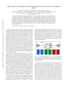
2.4 Calculating positions 2.4.1 Using the C/A code To start off, the receiver picks which C/A [1, 2] codes to listen for by PRN number, based on the almanac information it has previously acquired. As it detects each satellite's signal, it identifies it by its distinct C/A code pattern, then measures the received time for each satellite. To do this, the receiver produces an identical C/A sequence using the same seed number, referenced to its local clock, starting at the same time the satellite sent it. It then computes the offset to the local clock that generates the maximum correlation. This offset is the time delay from the satellite to the receiver, as told by the receiver's clock. Since the PRN repeats every millisecond, this offset is precise but ambiguous, and the ambiguity is resolved by looking at the data bits, which are sent at 50 Hz (20 ms) and aligned with the PRN code. This data is used to solve for x,y,z and t. Many mathematical techniques can be used. The following description shows a straightforward iterative way, but receivers use more sophisticated methods. (see Figure 2.1 below) Conceptually, the receiver calculates the distance to the satellite, called the pseudorange.
Figure2.1: Calculating position Overlapping pseudoranges, represented as curves, are modified to yield the probable position Next, the orbital position data, or ephemeris, from the Navigation Message is then downloaded to calculate the satellite's precise position. A more-sensitive receiver ٨
will potentially acquire the ephemeris data more quickly than a less-sensitive receiver, especially in a noisy environment. Knowing the position and the distance of a satellite indicates that the receiver is located somewhere on the surface of an imaginary sphere centered on that satellite and whose radius is the distance to it. Receivers can substitute altitude for one satellite, which the GPS receiver translates to a pseudorange measured from the center of the Earth. When pseudoranges have been determined for four satellites, a guess of the receiver's location is calculated. Dividing the speed of light by the distance adjustment required to make the pseudoranges come as close as possible to intersecting results in a guess of the difference between UTC and the time indicated by the receiver's on-board clock. With each combination of four satellites, a geometric dilution of precision (GDOP) vector is calculated, based on the relative sky positions of the satellites used. As more satellites are picked up, pseudoranges from more combinations of four satellites can be processed to add more guesses to the location and clock offset. The receiver then determines which combinations to use and how to calculate the estimated position by determining the weighted average of these positions and clock offsets. After the final location and time are calculated, the location is expressed in a specific coordinate system, e.g. latitude/longitude, using the WGS 84 geodetic datum or a local system specific to a country. There are many other alternatives and improvements to this process. If at least 4 satellites are visible, see Figure 2 for example, the receiver can eliminate time from the equations by computing only time differences, then solving for position as the intersection of hyperboloids. Also, with a full constellation and modern receivers, more than 4 satellites can be seen and received at once. Then all satellite data can be weighted by GDOP, signal to noise, path length through the ionosphere, and other accuracy concerns, and then used in a least squares fit to find a solution. In this case the residuals also gives an estimate of the errors. Finally, results from other positioning systems such as GLONASS or the upcoming Galileo can be used in the fit, or used to double-check the result. (By design, these systems use the same bands, so much of the receiver circuitry can be shared, though the decoding is different).
٩
2.4.2 Using the P(Y) code Calculating a position with the P(Y) [1, 2] signal is generally similar in concept, assuming one can decrypt it. The encryption is essentially a safety mechanism: if a signal can be successfully decrypted, it is reasonable to assume it is a real signal being sent by a GPS satellite. In comparison, civil receivers are highly vulnerable to spoofing since correctly formatted C/A signals can be generated using readily available signal generators. RAIM features do not protect against spoofing, since RAIM only checks the signals from a navigational perspective.
2.5 How accurate is GPS? Today's GPS receivers are extremely accurate, thanks to their parallel multichannel design. Garmin's 12 parallel channel receivers are quick to lock onto satellites when first turned on and they maintain strong locks, even in dense foliage or urban settings with tall buildings. Certain atmospheric factors and other sources of error can affect the accuracy of GPS receivers. Garmin® GPS receivers are accurate to within 15 meters on average [8]. Newer Garmin GPS receivers with WAAS (Wide Area Augmentation System) capability can improve accuracy to less than three meters on average. No additional equipment or fees are required to take advantage of WAAS. Users can also get better accuracy with Differential GPS (DGPS), which corrects GPS signals to within an average of three to five meters. The U.S. Coast Guard operates the most common DGPS correction service. This system consists of a network of towers that receive GPS signals and transmit a corrected signal by beacon transmitters. In order to get the corrected signal, users must have a differential beacon receiver and beacon antenna in addition to their GPS [1, 2].
2.5.1 Accuracy and error sources The position calculated by a GPS receiver requires the current time, the position of the satellite and the measured delay of the received signal. The position accuracy is ١٠
primarily dependent on the satellite position and signal delay.To measure the delay, the receiver compares the bit sequence received from the satellite with an internally generated version. By comparing the rising and trailing edges of the bit transitions, modern electronics can measure signal offset to within about 1% of a bit time, or approximately 10 nanoseconds for the C/A code. Since GPS signals propagate at the speed of light, this represents an error of about 3 meters. This is the minimum error possible using only the GPS C/A signal [1, 2, 7, 8]. Position accuracy can be improved by using the higher-chiprate P(Y) signal. Assuming the same 1% bit time accuracy, the high frequency P(Y) signal results in an accuracy of about 30 centimeters.Electronics errors are one of several accuracydegrading effects outlined in the table below. When taken together, autonomous civilian GPS horizontal position fixes are typically accurate to about 15 meters (50 ft). These effects also reduce the more precise P(Y) code's accuracy show Table 2.1 [7,8].
Sources of User Equivalent Range Errors (UERE) Source
Effect
Ionospheric effects
± 5 meter
Ephemeris errors
± 2.5 meter
Satellite clock errors
± 2 meter
Multipath distortion
± 1 meter
Tropospheric effects
± 0.5 meter
Numerical errors
± 1 meter
Table 2.1: Accuracy and error sources
١١
2.5.1.1 Atmospheric effects Inconsistencies of atmospheric conditions affect the speed of the GPS signals as they pass through the Earth's atmosphere, especially the ionosphere. Correcting these errors is a significant challenge to improving GPS position accuracy. These effects are smallest when the satellite is directly overhead and become greater for satellites nearer the horizon since the path through the atmosphere is longer (see airmass). Once the receiver's approximate location is known, a mathematical model can be used to estimate and compensate for these errors [1, 2]. Because ionospheric delay affects the speed of microwave signals differently depending on their frequency — a characteristic known as dispersion - delays measured on two more frequency bands can be used to measure dispersion, and this measurement can be then be used to estimate the delay at each frequency. Some military and expensive survey-grade civilian receivers measure the different delays in the L1 and L2 frequencies to measure atmospheric dispersion, and apply a more precise correction. This can be done in civilian receivers without decrypting the P(Y) signal carried on L2, by tracking the carrier wave instead of the modulated code. To facilitate this on lower cost receivers, a new civilian code signal on L2, called L2C, was added to the Block IIR-M satellites, which was first launched in 2005. It allows a direct comparison of the L1 and L2 signals using the coded signal instead of the carrier wave [1, 7, 8]. The effects of the ionosphere generally change slowly, and can be averaged over time. The effects for any particular geographical area can be easily calculated by comparing the GPS-measured position to a known surveyed location. This correction is also valid for other receivers in the same general location. Several systems send this information over radio or other links to allow L1-only receivers to make ionospheric corrections. The ionospheric data are transmitted via satellite in Satellite Based Augmentation Systems such as WAAS, which transmits it on the GPS frequency using a special pseudo-random noise sequence (PRN), so only one receiver and antenna are required. Humidity also causes a variable delay, resulting in errors similar to ionospheric delay, but occurring in the troposphere. This effect both is more localized and ١٢
changes more quickly than ionospheric effects, and is not frequency dependent. These traits make precise measurement and compensation of humidity errors more difficult than ionospheric effects. Changes in receiver altitude also change the amount of delay, due to the signal passing through less of the atmosphere at higher elevations. Since the GPS receiver computes its approximate altitude, this error is relatively simple to correct, either by applying a function regression or correlating margin of atmospheric error to ambient pressure using a barometric altimeter. 2.5.1.2 Multipath effects GPS signals can also be affected by multipath issues, where the radio signals reflect off surrounding terrain; buildings, canyon walls, hard ground, etc. These delayed signals can cause inaccuracy. A variety of techniques, most notably narrow correlator spacing, have been developed to mitigate multipath errors. For long delay multipath, the receiver itself can recognize the wayward signal and discard it. To address shorter delay multipath from the signal reflecting off the ground, specialized antennas (e.g. a choke ring antenna) may be used to reduce the signal power as received by the antenna. Short delay reflections are harder to filter out because they interfere with the true signal, causing effects almost indistinguishable from routine fluctuations in atmospheric delay [6, 7, 8]. Multipath effects are much less severe in moving vehicles. When the GPS antenna is moving, the false solutions using reflected signals quickly fail to converge and only the direct signals result in stable solutions. 2.5.1.3 Ephemeris and clock errors While the ephemeris data is transmitted every 30 seconds, the information itself may be up to two hours old. Data up to four hours old is considered valid for calculating positions, but may not indicate the satellites actual position. The satellite's atomic clocks experience noise and clock drift errors. The navigation message contains corrections for these errors and estimates of the accuracy of the atomic clock, however they are based on observations and may not indicate the ١٣
clock's current state.These problems tend to be very small, but may add up to a few meters (10s of feet) of inaccuracy [5]. 2.5.1.4 Selective availability GPS includes a (currently disabled) feature called Selective Availability (SA) that can introduce intentional, slowly changing random errors of up to a hundred meters (328 ft) into the publicly available navigation signals to confound, for example, guiding long range missiles to precise targets. When enabled, the accuracy is still available in the signal, but in an encrypted form that is only available to the United States military, its allies and a few others, mostly government users. Even those who have managed to acquire military GPS receivers would still need to obtain the daily key, whose dissemination is tightly controlled [1, 2]. Prior to being turned off, SA typically added signal errors of up to about 10 meters (32 ft) horizontally and 30 meters (98 ft) vertically. The inaccuracy of the civilian signal was deliberately encoded so as not to change very quickly. For instance, the entire eastern U.S. area might read 30 m off, but 30 m off everywhere and in the same direction. To improve the usefulness of GPS for civilian navigation, Differential GPS was used by many civilian GPS receivers to greatly improve accuracy [1]. During the Gulf War, the shortage of military GPS units and the ready availability of civilian ones caused many troops to buy their own civilian GPS units: their wide use among personnel resulted in a decision to disable Selective Availability. This was ironic, as SA had been introduced specifically for these situations, allowing friendly troops to use the signal for accurate navigation, while at the same time denying it to the enemy—but the assumption underlying this policy was that all U.S. troops and enemy troops would have military-specification GPS receivers and that civilian receivers would not exist in war zones. But since many American soldiers were using civilian devices, SA was also denying the same accuracy to thousands of friendly troops; turning it off (by removing the added-in error) presented a clear benefit to friendly troops.
١٤
In the 1990s, the FAA started pressuring the military to turn off SA permanently. This would save the FAA millions of dollars every year in maintenance of their own radio navigation systems. The amount of error added was "set to zero" at midnight on May 1, 2000 following an announcement by U.S. President Bill Clinton, allowing users access to the error-free L1 signal. Per the directive, the induced error of SA was changed to add no error to the public signals (C/A code). Clinton's executive order required SA to be set to zero by 2006; it happened in 2000 once the US military developed a new system that provides the ability to deny GPS (and other navigation services) to hostile forces in a specific area of crisis without affecting the rest of the world or its own military systems. Selective Availability is still a system capability of GPS, and error could, in theory, be reintroduced at any time. In practice, in view of the hazards and costs this would induce for US and foreign shipping, it is unlikely to be reintroduced, and various government agencies, including the FAA, have stated that it is not intended to be reintroduced. One interesting side effect of the Selective Availability hardware is the capability to correct the frequency of the GPS cesium and rubidium atomic clocks to an accuracy of approximately 2 × 10-13 (one in five trillion). This represented a significant improvement over the raw accuracy of the clocks.[citation needed] On 19 September 2007, the United States Department of Defense announced that future GPS III satellites will not be capable of implementing SA,[22] eventually making the policy permanent. 2.5.1.5 Relativity According to the theory of relativity, due to their constant movement and height relative to the Earth-centered inertial reference frame, the clocks on the satellites are affected by their speed (special relativity) as well as their gravitational potential (general relativity). For the GPS satellites, general relativity predicts that the atomic clocks at GPS orbital altitudes will tick more rapidly, by about 45.9 microseconds (µs) per day, because they are in a weaker gravitational field than atomic clocks on Earth's surface. Special relativity predicts that atomic clocks ١٥
moving at GPS orbital speeds will tick more slowly than stationary ground clocks by about 7.2 µs per day. When combined, the discrepancy is about 38 microseconds per day; a difference of 4.465 parts in 1010. To account for this, the frequency standard onboard each satellite is given a rate offset prior to launch, making it run slightly slower than the desired frequency on Earth; specifically, at 10.22999999543 MHz instead of 10.23 MHz. Since the atomic clocks on board the GPS satellites are precisely tuned, it makes the system a practical engineering application of the scientific theory of relativity in a real-world environment [1, 2, 7, 8]. 2.5.1.6 Sagnac distortion GPS observation processing must also compensate for the Sagnac effect. The GPS time scale is defined in an inertial system but observations are processed in an Earth-centered, Earth-fixed (co-rotating) system, a system in which simultaneity is not uniquely defined. A Lorentz transformation is thus applied to convert from the inertial system to the ECEF system. The resulting signal run time correction has opposite algebraic signs for satellites in the Eastern and Western celestial hemispheres. Ignoring this effect will produce an east-west error on the order of hundreds of nanoseconds, or tens of meters in position [1, 2].
2.5.2 GPS interference and jamming 2.5.2.1 Natural sources Since GPS signals at terrestrial receivers tend to be relatively weak, it is easy for other sources of electromagnetic radiation to desensitize the receiver, making acquiring and tracking the satellite signals difficult or impossible. Solar flares are one such naturally occurring emission with the potential to degrade GPS reception, and their impact can affect reception over the half of the Earth facing the sun. GPS signals can also be interfered with by naturally occurring geomagnetic storms, predominantly found near the poles of the Earth's magnetic field.GPS signals are also subjected to interference from Van Allen Belt radiation when the satellites pass through the South Atlantic Anomaly [1, 2].
١٦
2.5.1.2 Artificial sources Metallic features in windshields, such as defrosters, or car window tinting films can act as a Faraday cage, degrading reception just inside the car. Man-made EMI can also disrupt, or jam, GPS signals. In one well documented case, an entire harbor was unable to receive GPS signals due to unintentional jamming caused by a malfunctioning TV antenna preamplifier. Intentional jamming is also possible. Generally, stronger signals can interfere with GPS receivers when they are within radio range, or line of sight. In 2002, a detailed description of how to build a short range GPS L1 C/A jammer was published in the online magazine Phrack. The U.S. government believes that such jammers were used occasionally during the 2001 war in Afghanistan and the U.S. military claimed to destroy a GPS jammer with a GPS-guided bomb during the Iraq War.Such a jammer is relatively easy to detect and locate, making it an attractive target for anti-radiation missiles. The UK Ministry of Defence tested a jamming system in the UK's West Country on 7 and 8 June 2007. Some countries allow the use of GPS repeaters to allow for the reception of GPS signals indoors and in obscured locations, however, under EU and UK laws, the use of these is prohibited as the signals can cause interference to other GPS receivers that may receive data from both GPS satellites and the repeater. Due to the potential for both natural and man-made noise, numerous techniques continue to be developed to deal with the interference. The first is to not rely on GPS as a sole source. According to John Ruley, "IFR pilots should have a fallback plan in case of a GPS malfunction". Receiver Autonomous Integrity Monitoring (RAIM) is a feature now included in some receivers, which is designed to provide a warning to the user if jamming or another problem is detected. The U.S. military has also deployed their Selective Availability / Anti-Spoofing Module (SAASM) in the Defense Advanced GPS Receiver (DAGR). In demonstration videos, the DAGR is able to detect jamming and maintain its lock on the encrypted GPS signals during interference which causes civilian receivers to lose lock [1, 2].
١٧
2.6 Techniques to improve accuracy 2.6.1 Augmentation Augmentation methods of improving accuracy rely on external information being integrated into the calculation process. There are many such systems in place and they are generally named or described based on how the GPS sensor receives the information. Some systems transmit additional information about sources of error (such as clock drift, ephemeris, or ionospheric delay), others provide direct measurements of how much the signal was off in the past, while a third group provide additional navigational or vehicle information to be integrated in the calculation process.Examples of augmentation systems include the Wide Area Augmentation System, Differential GPS, Inertial Navigation Systems and Assisted GPS [7, 8].
2.6.2 Precise monitoring The accuracy of a calculation can also be improved through precise monitoring and measuring of the existing GPS signals in additional or alternate ways.After SA, which has been turned off, the largest error in GPS is usually the unpredictable delay through the ionosphere. The spacecraft broadcast ionospheric model parameters, but errors remain. This is one reason the GPS spacecraft transmit on at least two frequencies, L1 and L2. Ionospheric delay is a well-defined function of frequency and the total electron content (TEC) along the path, so measuring the arrival time difference between the frequencies determines TEC and thus the precise ionospheric delay at each frequency [7, 8]. Receivers with decryption keys can decode the P(Y)-code transmitted on both L1 and L2. However, these keys are reserved for the military and "authorized" agencies and are not available to the public. Without keys, it is still possible to use a codeless technique to compare the P(Y) codes on L1 and L2 to gain much of the same error information. However, this technique is slow, so it is currently limited to specialized surveying equipment. In the future, additional civilian codes are expected to be transmitted on the L2 and L5 frequencies (see GPS modernization, below). Then all
١٨
users will be able to perform dual-frequency measurements and directly compute ionospheric delay errors. A second form of precise monitoring is called Carrier-Phase Enhancement (CPGPS). The error, which this corrects, arises because the pulse transition of the PRN is not instantaneous, and thus the correlation (satellite-receiver sequence matching) operation is imperfect. The CPGPS approach utilizes the L1 carrier wave, which has a period 1000 times smaller than that of the C/A bit period, to act as an additional clock signal and resolve the uncertainty. The phase difference error in the normal GPS amounts to between 2 and 3 meters (6 to 10 ft) of ambiguity. CPGPS working to within 1% of perfect transition reduces this error to 3 centimeters (1 inch) of ambiguity. By eliminating this source of error, CPGPS coupled with DGPS normally realizes between 20 and 30 centimeters (8 to 12 inches) of absolute accuracy. Relative Kinematic Positioning (RKP) is another approach for a precise GPS-based positioning system. In this approach, determination of range signal can be resolved to a precision of less than 10 centimeters (4 in). This is done by resolving the number of cycles in which the signal is transmitted and received by the receiver. This can be accomplished by using a combination of differential GPS (DGPS) correction data, transmitting GPS signal phase information and ambiguity resolution techniques via statistical tests—possibly with processing in real-time (real-time kinematic positioning, RTK).
2.6.3 GPS time and date While most clocks are synchronized to Coordinated Universal Time (UTC), the atomic clocks on the satellites are set to GPS time. The difference is that GPS time is not corrected to match the rotation of the Earth, so it does not contain leap seconds or other corrections which are periodically added to UTC. GPS time was set to match Coordinated Universal Time (UTC) in 1980, but has since diverged. The lack of corrections means that GPS time remains at a constant offset (19 seconds) with International Atomic Time (TAI). Periodic corrections are performed on the onboard clocks to correct relativistic effects and keep them synchronized with ground clocks [1, 2].
١٩
The GPS navigation message includes the difference between GPS time and UTC, which as of 2006 is 14 seconds due to the leap second added to UTC December 31st of 2005. Receivers subtract this offset from GPS time to calculate UTC and specific timezone values. New GPS units may not show the correct UTC time until after receiving the UTC offset message. The GPS-UTC offset field can accommodate 255 leap seconds (eight bits) which, at the current rate of change of the Earth's rotation, is sufficient to last until the year 2330. As opposed to the year, month, and day format of the Gregorian calendar, the GPS date is expressed as a week number and a day-of-week number. The week number is transmitted as a ten-bit field in the C/A and P(Y) navigation messages, and so it becomes zero again every 1,024 weeks (19.6 years). GPS week zero started at 00:00:00 UTC (00:00:19 TAI) on January 6, 1980 and the week number became zero again for the first time at 23:59:47 UTC on August 21, 1999 (00:00:19 TAI on August 22, 1999). To determine the current Gregorian date, a GPS receiver must be provided with the approximate date (to within 3,584 days) to correctly translate the GPS date signal. To address this concern the modernized GPS navigation messages use a 13-bit field, which only repeats every 8,192 weeks (157 years), and will not return to zero until near the year 2137.
2.6.4 GPS modernization Having reached the program's requirements for Full Operational Capability (FOC) on July 17, 1995, the GPS completed its original design goals. However, additional advances in technology and new demands on the existing system led to the effort to modernize the GPS. Announcements from the Vice President and the White House in 1998 initiated these changes, and in 2000 the U.S. Congress authorized the effort, referring to it as GPS III [1, 2]. The project aims to improve the accuracy and availability for all users and involves new ground stations, new satellites, and four additional navigation signals. New civilian signals are called L2C, L5 and L1C; the new military code is called M-Code. Initial Operational Capability (IOC) of the L2C code is expected in 2008. A goal of 2013 has been established for the entire program, with incentives offered to the contractors if they can complete it by 2011. ٢٠
2.7 Applications The Global Positioning System, while originally a military project, is considered a dual-use technology, meaning it has significant applications for both the military and the civilian industry. There are many application show Figure 2.2 [6].
Figure 2.2: GPS Applications
2.7.1 Military The military applications of GPS span many purposes [3]: •
Navigation: GPS allows soldiers to find objectives in the dark or in unfamiliar territory, and to coordinate the movement of troops and supplies. The GPS-receivers commanders and soldiers use are respectively called the Commanders Digital Assistant and the Soldier Digital Assistant.
•
Target tracking: Various military weapons systems use GPS to track potential ground and air targets before they are flagged as hostile. These weapon systems pass GPS co-ordinates of targets to precision-guided munitions to allow them to engage the targets accurately. Military aircraft, particularly those used in air-to-ground roles use GPS to find targets (for example, gun camera video from AH-1 Cobras in Iraq show GPS co-ordinates that can be looked up in Google Earth).
•
Missile and projectile guidance: GPS allows accurate targeting of various military weapons including ICBMs, cruise missiles and precision-guided munitions. Artillery projectiles with embedded GPS receivers able to ٢١
withstand accelerations of 12,000G have been developed for use in 155 mm howitzers. •
Search and Rescue: Downed pilots can be located faster if they have a GPS receiver.
•
Reconnaissance and Map Creation: The military use GPS extensively to aid mapping and reconnaissance.
•
The GPS satellites also carry a set of nuclear detonation detectors consisting of an optical sensor (Y-sensor), an X-ray sensor, a dosimeter, and an ElectroMagnetic Pulse (EMP) sensor (W-sensor) which form a major portion of the United States Nuclear Detonation Detection System.
2.7.2 Civilian This antenna is mounted on the roof of a hut containing a scientific experiment needing precise timing.Many civilian applications benefit from GPS signals, using one or more of three basic components of the GPS: absolute location, relative movement, and time transfer.The ability to determine the receiver's absolute location allows GPS receivers to perform as a surveying tool or as an aid to navigation. The capacity to determine relative movement enables a receiver to calculate local velocity and orientation, useful in vessels or observations of the Earth. Being able to synchronize clocks to exacting standards enables time transfer, which is critical in large communication and observation systems. An example is CDMA digital cellular. Each base station has a GPS timing receiver to synchronize its spreading codes with other base stations to facilitate inter-cell hand off and support hybrid GPS/CDMA positioning of mobiles for emergency calls and other applications. Finally, GPS enables researchers to explore the Earth environment including the atmosphere, ionosphere and gravity field. GPS survey equipment has revolutionized tectonics by directly measuring the motion of faults in earthquakes [1, 2]. To help prevent civilian GPS guidance from being used in an enemy's military or improvised weaponry, the US Government controls the export of civilian receivers. ٢٢
A US-based manufacturer cannot generally export a GPS receiver unless the receiver contains limits restricting it from functioning when it is simultaneously (1) at an altitude above 18 kilometers (60,000 ft) and (2) traveling at over 515 m/s (1,000 knots). These parameters are well above the operating characteristics of the typical cruise missile, but would be characteristic of the reentry vehicle from a ballistic missile. GPS functionality has now started to move into mobile phones en masse. Although the first GSM handsets with integrated GPS were launched already in the late 1990’s, broader availability of consumer-oriented handsets with GPS did not appear until late 2006, primarily in Japan. Outside Japan, numerous smartphone vendors have introduced handsets with GPS during 2007. Moreover, the largest handset vendor in the world, Nokia, accelerated its LBS initiative by acquiring the leading digital map provider NAVTEQ. In response to increasing interest in location-based services, as well as to comply with regulations, all major handset vendors have now presented GPS-enabled GSM/WCDMA handsets. Who uses GPS? GPS has a variety of applications on land, at sea and in the air. Basically, GPS is usable everywhere except where it's impossible to receive the signal such as inside most buildings, in caves and other subterranean locations, and underwater. The most common airborne applications are for navigation by general aviation and commercial aircraft. At sea, GPS is also typically used for navigation by recreational boaters, commercial fishermen, and professional mariners. Land-based applications are more diverse. The scientific community uses GPS for its precision timing capability and position information. Surveyors use GPS for an increasing portion of their work. GPS offers cost savings by drastically reducing setup time at the survey site and providing incredible accuracy. Basic survey units, costing thousands of dollars, can offer accuracies down to one meter. More expensive systems are available that can provide accuracies to within a centimeter. Recreational uses of GPS are almost as varied as the number of recreational sports available. GPS is popular among hikers, hunters, snowmobilers, mountain bikers, and cross-country skiers, just to name a few. Anyone who needs to keep track of ٢٣
where he or she is, to find his or her way to a specified location, or know what direction and how fast he or she is going can utilize the benefits of the global positioning system. GPS is now commonplace in automobiles as well. Some basic systems are in place and provide emergency roadside assistance at the push of a button (by transmitting your current position to a dispatch center). More sophisticated systems that show your position on a street map are also available. Currently these systems allow a driver to keep track of where he or she is and suggest the best route to follow to reach a designated location.
٢٤
Chapter 3 GPS Tracking and Detecting
3.1 Introduction A GPS tracking unit is a device that uses the Global Positioning System to determine the precise location of a vehicle, person, or other asset to which it is attached and to record the position of the asset at regular intervals. The recorded location data can be stored within the tracking unit, or it may be transmitted to a central location data base, or internet-connected computer, using a cellular (GPRS), radio, or satellite modem embedded in the unit. This allows the asset's location to be displayed against a map backdrop either in real-time or when analyzing the track later, using customized software [10, 11]. Such systems are not new; amateur radio operators have been operating their free GPS based nationwide real time Automatic Position Reporting System since 1982. The new GPS auto tracker technology allows just about anyone to track anyone else.
3.2 Types of GPS trackers Two types of GPS tracking device technology available to the public [12]: •
passive or logger tracking device.
•
real time tracking devices(active).
3.2.1 Passive Tracking Passive GPS tracking is also a system for monitoring an offender's movement and compliance data 24/7, anywhere in the world. Each passive GPS device continuously records location data throughout the day and is programmable to remember zones that are off-limits (schools or a spouse's residence, for example). Each unit can also remember the areas an offender is required to be in at certain times (at work from 8:00 AM to 5:00 PM and at diversion sessions on Tuesdays from ٢٥
6:00 PM to 7:00 PM, for example). If the offender isn't compliant to these parameters, passive GPS unit will note a violation [12, 13]. A passive unit transmits updated tracking information less frequently than an active GPS device does - normally at the end of the day. Authorized personnel can then see updated information once the data has been transferred. Most passive systems transmit data over regular phone lines rather than through cellular networks. This ability to utilize land-lines is necessary for many agencies covering rural or remote areas where cellular coverage may be inadequate. Passive systems also cost less than active systems and are ideal for agencies that don't require immediate notifications. 3.2.1.1 How does it work? Our passive GPS unit tracks the individual every 10 seconds and remembers the person's boundaries and stipulations as set by the government agency, illustrate in Figure 3.1. Passive unit also has an on-board processor which immediately detects and records when the individual is in violation, but the passive unit doesn't contact the data center at once. When the offender places the unit in the charging base (usually when he returns home for the day), the unit calls our data center and transfers the day's information. The corresponding officer can then use any PC connected to the Internet (no additional software required) to connect to tracNET24 and access offender tracking, violation, and compliance information.
Figure 3.1: Passive tracking Since tracking points are recorded every 10 seconds, criminal justice personnel can review animated offender movement in the finest detail possible, complete with time/date stamps and velocity information. This is extraordinarily useful when an
٢٦
offender is in a vehicle and can dramatically change locations in less than 60 seconds. 3.2.1.2 Does it save you time?
Absolutely. Since our passive GPS system is exception-based, it streamlines your workload, rather than adding to it. Our system only gives you the information you find helpful. 3.2.1.3 How can this help you? •
Know where your offenders have been after they've left the house
•
Focus your supervision on those who really need supervision
•
Manage large caseloads in less time
•
Increase accountability and compliance
3.2.1.4 What makes ours the best on the market? •
Easiest to use
•
Most advanced
•
Most dependable performance in the field
3.2.2 GPS Tracking Active GPS tracking is a system for monitoring an individual's movement and compliance to time/location parameters 24/7/365, anywhere in the world. GPS tracking is sometimes also referred to as GPS location verification. An Active GPS device has the ability to use wireless communications to send offender data to a central data center, enabling an officer to receive updated information (locations and violations) throughout the day, illustrate in Figure 3.2. [12, 13]. Each active GPS unit is programmable to remember zones that are off-limits (schools or a spouse's residence, for example). Each unit can also remember the areas an ٢٧
offender is required to be in at certain times (at work from 8:00 AM to 5:00 PM and at diversion sessions on Tuesdays from 6:00 PM to 7:00 PM, for example). If the offender isn't compliant to these parameters, active GPS unit will note a violation and can send an alert. 3.2.2.1 How does it work? The active GPS unit tracks an individual every 10 seconds and also has a copy of the offender's time/location parameters. The tracking unit not only records GPS points, but it also cross-checks parameters and realizes when the offender has committed a violation. This is known as on-board processing and is what gives active systems the fastest response time of anything in the industry. As soon as the individual is in violation, the GPS unit attempts to communicate with tracNET24 over a cellular network. tracNET24 alerts the government agency, makes the information available online, and stores offender information for the long term. The corresponding officer can then use most any PC connected to the Internet (no additional software required) to see where the offender has been and when he was there. Our website provides agencies with updated offender information in easy-tounderstand formats - maps, violations, tampers with equipment, reports, and more.
Figure 3.2: Real Tracking
٢٨
3.2.2.2 Does it save you time? Absolutely. Since our active GPS system is exception-based, it streamlines your workload, rather than adding to it. Our system only gives you the information you find helpful. 3.2.2.3 How can this help you? •
Know where your offenders have been after they've left the house
•
Focus your supervision on those who really need supervision
•
Manage large caseloads in less time
•
Increase accountability and compliance
3.2.2.4 What makes ours the best on the market? •
Easiest to use
•
Most advanced
•
Most dependable performance in the field
3.3 Categories of GPS trackers Usually, a GPS tracker will fall into one of these three categories: 1. Data loggers 2. Data pushers 3. Data pullers
3.3.1 Data loggers A GPS logger [13, 14] simply logs the position of the device at regular intervals in its internal memory. Modern GPS loggers have either a memory card slot, or internal flash memory and a USB port. Some act as a USB flash drive. This allows downloading of the data for further analysis in a computer.
٢٩
These kind of devices are most suited for use by sport enthusiasts: They carry it while practising an outdoors sport, e.g. jogging or backpacking. When they return home, they download the data to a computer, to calculate the length and duration of the trip, or to overimpose their paths over a map with the aid of GIS software. GPS devices are also integral tools in geocaching. In the sport of gliding, competitors are sent to fly over closed circuit tasks of hundreds of kilometres. GPS loggers are used to prove that the competitors completed the task and stayed away from controlled airspace. The data stored over many hours in the loggers is downloaded after the flight is completed and is analysed by computing the start and finish times so determining the fastest competitors. In some Private Investigation cases, these data loggers are used to keep track of the vehicle or the fleet vehicle. The reason for using this device is so that a PI will not have to follow the target so closely and always has a backup source of data.
3.3.2 Data pushers This is the kind of devices used by the security industry, which pushes (i.e. "sends") the position of the device, at regular intervals, to a determined server, that can instantly analyze the data. These devices started to become popular and cheaper at the same time as mobile phones. The falling prices of the SMS services, and smaller sizes of phone allowed to integrate the technologies at a fair price. A GPS receiver and a mobile phone sit side-by-side in the same box, powered by the same battery. At regular intervals, the phone sends a text message via SMS, containing the data from the GPS receiver. Some companies provide data "push" technology, enabling sophisticated GPS tracking in business environments, specifically organizations that employ a mobile workforce, such as a commercial fleet.The applications of these kind of trackers include:Fleet control. For example, a delivery or taxi company may put such a tracker in every of its vehicles, thus allowing the staff to know if a vehicle is on time or late, or is doing its assigned route. The same applies for armored trucks transporting valuable goods, as it allows to pinpoint the exact site of a possible robbery [13, 14].
٣٠
Stolen vehicle searching. Owners of expensive cars can put a tracker in it, and "activate" them in case of theft. "Activate" means that a command is issued to the tracker, via SMS or otherwise, and it will start acting as a fleet control device, allowing the user to know where the thieves are. Animal control. When put on a wildlife animal (e.g. in a collar), it allows scientists to study its activities and migration patterns. Vaginal implant transmitters are used to mark the location where pregnant females give birth.[1] Animal tracking collars may also be put on domestic animals, to locate them in case they get lost. Race control. In some sports, such as gliding, participants are required to have a tracker with them. This allows, among other applications, for race officials to know if the participants are cheating, taking unexpected shortcuts or how far apart they are. This use has been featured in the movie "Rat Race", where some millionaires see the position of the racers in a wall map. Espionage/surveillance. When put on a person, or on his personal vehicle, it allows the person monitoring the tracking to know his/her habits. This application is used by private investigators, and also by some parents to track their children. Internet Fun. Some Web 2.0 pioneers have created their own personal web pages that show their position constantly, and in real-time, on a map within their website. These usually use data push from a GPS enabled cell phone.
3.3.3 Data pullers Contrary to a data pusher, that sends the position of the device at regular intervals (push technology), these devices are always-on and can be queried as often as required (pull technology). This technology is not in widespread use, but an example of this kind of device is a computer connected to the Internet and running gpsd. These can often be used in the case where the location of the tracker will only need to be known occasionally e.g. placed in property that may be stolen.
٣١
Data Pullers are coming into more common usage in the form of devices containing a GPS receiver and a cell phone which, when sent a special SMS message reply to the message with their location [13, 14].
3.4 Potential abuse of GPS trackers In the US, the use of GPS trackers by police requires a search warrant in some circumstances, but use by a private citizen does not, as the Fourth Amendment does not limit the actions of private citizens. These devices can also raise concerns about personal privacy. Over time, the information collected could reveal a typical pattern of movements.
3.5 Countermeasures against GPS trackers The consumer electronics market was quick to offer remedies (radar detectors) to radar guns; a similar market may exist for devices to counter satellite tracking devices. Radio jamming of the relevant GPS or cell phone frequencies would be an option, as would a device which could detect the RF emissions of the GPS receiver circuitry. However, jamming of GPS signals could create a safety hazard to vehicles or aircraft within line of sight of the jammer, and any deliberate radio interference is likely to be illegal in most Western countries[15, 16]. Besides this, jamming the transmission frequency of an industrial grade GPS transmitter would only work temporarily because most of them use a "store and forward" procedure to store up points that were not received and transmit them again later. This capability is built-in so tracked vehicles don't lose data when they are out of cellular range temporarily. Jamming the actual GPS frequency, however, would result in the GPS transmitter simply thinking it had lost sight of the satellites [15].
3.6 IS it Legal to use GPS Tracking Units? In most cases it is illegal to track just about anyone without their permission. However given the fact that is so hard to detect many tracking devices it is likely that illegal GPS auto tracker and personal tracking device technology will continue to be used. ٣٢
3.7 GPS Detecting It is possible to detect a GPS tracking [17, 18, 19, 20] device that transmits information by using a radio frequency detector/scanner. The problem is that the RF detector/scanner [21] will only detect the transmissions of the GPS device when the device is actually transmitting. This also notes that GPS devices use different technologies, which can also cause complications in detecting them. Another site follows up on that, explaining that some trackers do transmit a constant signal, which makes them easier to detect, and that the same is true of GPS devices that use cell phone connections. I say ultimately the best way to find a GPS device is to use a combination of detection
and
“finger-tip
٣٣
searching.”
Chapter 4 GPS Signal Structure
In order to design a software-defined [22, 23, 24, 25, 26] single frequency GPS receiver it is necessary to know the characteristics of the signal and data transmitted from the GPS satellites and received by the GPS receiver antenna. In this chapter an overview of the GPS signal generation scheme and the most important properties of the various signals and data are presented.
4.1 Signals and Data The GPS signals are transmitted on two radio frequencies in the UHF band. The UHF band covers the frequency band from 500MHz to 3GHz. These frequencies are referred to as L1 and L2 and are derived from a common frequency, f0 = 10.23MHz: fL1 = 154 f0 = 1575.42MHz, (2.1) fL2 = 120 f0 = 1227.60MHz. (2.2) The signals are composed of the following three parts: Carrier The carrier wave with frequency fL1 or fL2, Navigation data The navigation data contain information regarding satellite or- bits. This information is uploaded to all satellites from the ground stations in the GPS Control Segment. The navigation data have a bit rate of 50 bps, illustrate in Figure 4.1. [1, 2].
٣٤
Figure 4.1: GPS Signal Structure
Spreading sequence each satellite has two unique spreading sequences or codes. The first one is the coarse acquisition code (C/A), and the other one is the encrypted precision code (P(Y)). The C/A code is a sequence of 1023 chips. (A chip corresponds to a bit. It is simply called a chip to emphasize that it does not hold any information.) The code is repeated each ms giving a chipping rate of 1.023MHz. The P code is a longer code (≈ 2.35·104 chips) with a chipping rate of 10.23MHz. It repeats itself each week starting at the beginning of the GPS week which is at Saturday/Sunday midnight. The C/A code is only modulated onto the L1 carrier while the P(Y) code is modulated onto both the L1 and the L2 carrier. Section 2.3 describes the generation and properties of the spreading sequences in detail.
4.2 Coarse / Acquisition code The C/A [1, 2] code is a 1,023 bit long pseudorandom number (PRN) which, when transmitted at 1.023 megabits per second (Mbit/s), repeats every millisecond. Pseudorandom numbers only match up, or strongly correlate, when they are exactly aligned. Each satellite transmits a unique PRN code, which does not correlate well ٣٥
with any other satellite's PRN code. In other words, the PRN codes are highly orthogonal to one another. This is a form of Code Division Multiple Access (CDMA), which allows the receiver to recognize multiple satellites on the same frequency.
4.5 Precision code The P-code [1, 2] is also a PRN, however each satellite's P-code PRN code is 6.1871 × 1012 bits long (6,187,100,000,000 bits) and only repeats once a week (it is transmitted at 10.23 Mbit/s). The extreme length of the P-code increases its correlation gain and eliminates any range ambiguity within the Solar System. However, the code is so long and complex it was believed that a receiver could not directly acquire and synchronize with this signal alone. It was expected that the receiver would first lock onto the relatively simple C/A code and then, after obtaining the current time and approximate position, synchronize with the P-code. Whereas the C/A PRNs are unique for each satellite, the P-code PRN is actually a small segment of a master P-code approximately 2.35 × 1014 bits in length (235,000,000,000,000 bits) and each satellite repeatedly transmits its assigned segment of the master code. To prevent unauthorized users from using or potentially interfering with the military signal through a process called spoofing, it was decided to encrypt the P-code. To that end the P-code was modulated with the W-code, a special encryption sequence, to generate the Y-code. The Y-code is what the satellites have been transmitting since the anti-spoofing module was set to the "on" state. The encrypted signal is referred to as the P(Y)-code. The details of the W-code are kept secret, but it is known that it is applied to the Pcode at approximately 500 kHz, which is a slower rate than that of the P-code itself by a factor of approximately 20. This has allowed companies to develop semicodeless approaches for tracking the P(Y) signal, without knowledge of the W-code itself.
٣٦
4.4 Navigation message In addition to the PRN ranging codes, a receiver needs to know detailed information about each satellite's position and the network. The GPS design has this information modulated on top of both the C/A and P(Y) ranging codes at 50 bit/s and calls it the Navigation Message. The navigation message is made up of three major components. The first part contains the GPS date and time, plus the satellite's status and an indication of its health. The second part contains orbital information called ephemeris data and allows the receiver to calculate the position of the satellite. The third part, called the almanac, contains information and status concerning all the satellites; their locations and PRN numbers [1, 2, 27, 28, 29]. Whereas ephemeris information is highly detailed and considered valid for no more than four hours, almanac information is more general and is considered valid for up to 180 days. The almanac assists the receiver in determining which satellites to search for, and once the receiver picks up each satellite's signal in turn, it then downloads the ephemeris data directly from that satellite. A position fix using any satellite can not be calculated until the receiver has an accurate and complete copy of that satellite's ephemeris data. The navigation message itself is constructed from a 1,500 bit frame, which is divided into five subframes of 300 bits each and transmitted at 50 bit/s (therefore each subframe requires 6 seconds to transmit). Subframe 1 contains the GPS date and time, plus satellite status and health. Subframes 2 and 3, when combined, contain the transmitting satellite's ephemeris data. Subframes 4 and 5, when combined, contain 1/25th of the almanac; meaning 25 whole frames worth of data are required to complete the 15,000 bit almanac message. At this rate, 12.5 minutes are required to receive the entire almanac from a single satellite.
٣٧
4.5 Frequency information For the ranging codes and navigation message to travel from the satellite to the receiver, they must be modulated onto a carrier frequency. In the case of the original GPS design, two frequencies are utilized; one at 1575.42 MHz (10.23 MHz × 154) called L1; and a second at 1227.60 MHz (10.23 MHz × 120), called L2. The C/A code is transmitted on the L1 frequency as a 1.023 MHz signal using a BiPhase Shift Key (BPSK) modulation technique. The P(Y)-code is transmitted on both the L1 and L2 frequencies as a 10.23 MHz signal using the same BPSK modulation, however the P(Y)-code carrier is in quadrature with the C/A carrier; meaning it is 90° out of phase [1,2, 30]. Besides the redundancy and increased resistance to jamming, a critical benefit of having two frequencies transmitted from one satellite is the ability to directly measure, and therefore remove, the ionospheric delay error for that satellite. Without such a measurement, a GPS receiver must use a generic model or receive ionospheric corrections from another source (such as the Wide Area Augmentation System or EGNOS). Advances in the technology used on both the GPS satellites and the GPS receivers has made ionospheric delay the largest source of error in the signal. A receiver capable of performing this measurement can be significantly more accurate and is typically referred to as a dual frequency receiver.
4.6 GPS Signal Scheme In the following a detailed description of the signal generation is given. Figure 2.1 is a block diagram describing the signal generation .The block diagram should be read from left to right. At the far left, the main clock signal is supplied to the remaining blocks. The clock signal has a frequency of 10.23MHz. Actually, the exact frequency is 10.22999999543MHz to adjust for relativistic effects giving a frequency of 10.23MHz seen from the user on Earth.When multiplied by 154 and 120, it generates the L1 and L2 carrier signals, respectively. At the bottom left corner a limiter is used to stabilize the clock signal before supplying it to the P(Y) and C/A code generators. At the very bottom the data generator generates the navigation data.
٣٨
The code generators and the data generator are synchronized through the X1 signal supplied by the P(Y) code generator [2 ,31,32].
Table 4.1:Exclusive OR operation
Table 4.2: Ordinary multiplication
After code generation, the codes are combined with the navigation data through modulo-2 adders. The exclusive OR operation is used on binary sequences represented by 0’s and 1’s, and its properties are shown in Table 4.1 [33]. If the binary sequences were represented by the polar non-return-to-zero representation, i.e., 1’s and −1’s, ordinary multiplication could be used instead. The ٣٩
corresponding properties of the multiplication with two binary non-return-to-zero sequences are shown in Table 4.2. The C/A code data and the P(Y) code data signals are supplied to the two modulators for the L1 frequency. Here the signals are modulated onto the carrier signal using the binary phase shift keying (BPSK) method. Note that the two codes are modulated inphase and quadrature with each other on L1. That is, there is a 90◦ phase shift between the two codes. We return to this issue shortly. After the P(Y) part is attenuated 3 dB, these two L1 signals are added to form the resulting L1 signal. The so-called standard positioning service (SPS) is based on C/A code signals alone [34]. It follows that the signal transmitted from satellite k can be described as
where PC, PPL1,and PPL2 are the powers of signals with C/A or P code, Ck is the C/A code sequence assigned to satellite number k, Pk is the P(Y) code sequence assigned to satellite number k, Dk is the navigation data sequence, and fL1 and fL2 are the carrier frequencies of L1 and L2, respectively. Figure 4.2 shows the three parts forming the signal on the L1 frequency. The C/A code repeats itself every ms, and one navigation bit lasts 20ms. Hence for each navigation bit, the signal contains 20 complete C/A codes. Figure 4.2 shows the Gold code C, the navigation data D, the modulo-2 added signal C�D, and the carrier. The final signal is created by binary phase-shift keying (BPSK) where the carrier is instantaneously phase shifted by 180◦ at the time of a chip change. When a navigation data bit transition occurs (about one third from the right edge), the phase of the resulting signal is also phase-shifted 180◦.
٤٠
Figure 4.2: GPS Signal Coding
L1 signal structure is the carrier wave and C(t ) is the discrete C/A code sequence. As seen, this signal repeats itself every ms. D(t ) is the discrete navigation data bit stream. One navigation bit lasts 20ms. The three parts of the L1 signal are multiplied to form the resulting signal. This figure is not to scale but is only used for illustrative purpose [35, 36, 37]. For GPS the code length is 1023 chips, 1.023MHz chipping rate (1ms period time), 50Hz data rate (20 code periods per data bit), � 90%of signal power within 2MHz bandwidth.
٤١
Chapter 5 GPS Jamming Signal Issue
5.1 Definitions Most jamming techniques [38,39,40,41,42] fall into three major types usually based on bandwidth. Continuous wave, or CW jamming, is usually defined as occupying less than 100 kHz of bandwidth. In this paper, CW jamming will be defined as one frequency only. Narrowband (NB) jamming will be defined as any unwanted signal occupying more than one MHz of bandwidth but less than or equal to the entire ±1.023 MHz bandwidth of C/A code. NB is usually centered about L1 or L2 but not necessarily so. Wideband (WB) jamming will be defined as jamming signals occupying the entire ±10.23 MHz bandwidth about L1 or L2. All discussions of J/S will be related to dBm. J/S ratios are with respect to L1 or L2 P(Y) code only, where L1 = -133 dBm, L2 = -136 dBm. Three dB are added for C/A-code J/S comparisons.
5.2 Jamming Design Issues 5.2.1 Accuracy When testing GPS receivers/navigation systems, the most important jamming specification is the amplitude accuracy, because overall J/S is calculated using jamming signal amplitude. When measuring the GPS jamming signals, it is also important to note that the complete 20.46 MHz of signal bandwidth for L1 or L2 P(Y) code should be measured to ensure that all the jamming energy is accounted for when performing the J/S calculations. GPS simulator signals must also have correct signal power levels. Adjusting the power output to correct for the testing system's ٤٢
losses or gains usually attains this. Incorrect GPS simulator output levels will cause J/S to be artificially high or low, nullifying test results, even if the GPS jamming levels are correct. In order to validate the performance of the GPS component of any given platform in the Navigation Laboratory, we need to be able to determine J/S as accurately as possible. Any error in determining this parameter can have a large impact on system performance. For example, suppose we wish to determine how a +1.0 dB error in measuring the amplitude of jamming would affect the overall accuracy ofour J/S calculation. Assume there is no amplitude error in S, the GPS signal level, and that it is a constant value. Given 1 dB = 10 Log JM / JT where JM = Measured jammer power JT = True jammer power then JT = 1.26 JM or a positive 26% error in measurement. For a -1.0 dB error in measuring jamming amplitude, we have -1 dB = 10 Log JM / JT or
JT = 0.79 JM
which corresponds to a negative 21% error in our measurement. Another example relating measurement error to range follows. Suppose we wish to determine the range at which\ a given receiver loses lock for a fixed jammer power. Since power decreases as the reciprocal of the distance from the emitter, we have JM / JT = (RT /RM)
٤٣
where
RT = range calculated using JT RM = range calculated using JM This equation can be rewritten as 10 Log JM – 10 Log JT = 20 Log RT /RM If we assume a +1.0 dB error in measuring JM, we have RM = RT * 10 -1/20 or
RM = 0.89 RT
This represents an 11% error in our range estimate to jam- out, possibly a critical parameter of the system's operational design.
This error may translate into an
operational concern for certain customers. Based upon these brief calculations, it appears that the maximum amplitude measurement error we should allow for when performing GPS jamming is ±1.0 dB.
For reference, the Interstate Electronics
Corporation (IEC)3 GPS constellation simulator specifies an amplitude accuracy of ±0.7 dB root sum squared when generating satellite signals, on par with the previously stated accuracy requirement for jamming signals. The total amplitude error of J/S that exists when performing jamming testing will be made up of errors in both J and S. Amplitude errors in the simulator output S cannot be easily calibrated and reflect the performance specification of the GPS simulator. Amplitude errors in jamming or J can be minimized but not completely eliminated. To produce GPS jamming signals that have accuracy values similar to the simulator means generating jamming signals with less than ±0.7 dB of amplitude error. GPS receiver/system testing can be performed with or without the antenna or antenna subsystem. When testing with single-element or multi-element antennas, the requirement that all ٤٤
jamming be measured to within ±1.0dB is still valid. If jamming an actual antenna system in an anechoic chamber, a calibrated radio frequency (RF) horn or some other measurement device should be used to determine the actual power levels present at the antennaelements. When testing GPS receivers without the antenna, the signal specification for power at the input to the receiver must be accounted for. This signal level can be above or below ICD-GPS-200 levels. All system gains or losses must be accounted for to ensure the signal feeding the input to the receiver under test is correct in amplitude. If jamming a multi-element GPS receiver system without the antenna, then each RF input (one per antenna element) should be measured to within the previously mentioned ±1.0 dB value to ensure jamming levels are correct.
5.2.2 Frequency There are other important jamming parameters besides amplitude tolerances. Frequency is also an important issue. CW jammer or NB jammer center frequency location relative to the GPS signal is important, especially if testing a GPS receiver that can notch-out CW and NB jammers in the frequency domain. Too much drift from the commanded center frequency of the signal generators could nullify test results. From test experience, we have found that knowing the center frequency of any jamming to within ±500 Hz over the 20.46 MHz GPS bandwidth is accurate enough for laboratory testing. If needed, more accuracy could easily be obtained by feeding a highly accurate frequency standard into the laboratory signal generators. When generating jamming signals that can be moved about the entire bandwidth of GPS, care should be taken to limit the absolute frequency offset allowed to ensure that ٤٥
signals stay within the bandwidth. The front-end bandwidth of the GPS receiver under test and the accuracy of the signal generators usually determine the maximum allowable frequency offset. We chose to limit the frequency offset to ±9.0 MHz to avoid generating jamming outside the band, and to ensure that all the jamming energy enters the GPS receiver under test.
5.2.3 Pulse For pulse jamming (turning CW, NB, and WB jamming on and off at some rate), care should be taken to limit the two pulse description parameters, pulse repetition frequency (PRF) and duty cycle (DC). Large values for both PRF and DC will make the jamming look continuous, and very small values for both will not affect the GPS receiver noticeably.
Also, the ability of the test equipment to
accurately emulate any given pulse characteristics should be taken into account. Usually the rise and fall times of test equipment controlling the RF output of pulses is sufficiently fast enough (msec to nsec) that the pulse appears instantaneous to the GPS receiver(s) RF input. Realistic values found through experimentation are: Minimum PRF: 1 Hz, Maximum PRF: 20 kHz Minimum DC: 10%, Maximum DC: 90% These values should only be considered as a starting point and are tailorable for specific requirements.
5.2.4 Modulation/Mixing The overriding goal of any GPS jamming modulation/mixing scheme is to completely fill a given bandwidth of frequency with energy that will cause the GPS receiver to lose lock or never attain lock.There are many types of modulation options available. Some standard modulation types are amplitude modulation (AM), ٤٦
frequency modulation (FM), and biphase shift keying (BPSK). Mixing of noise with a carrier frequency to produce WB jamming is another common practice. Other options are as follows: sweeping the center frequency, summing two different kinds of modulation together (AM and FM, for instance), RF summation of multiple signal generator jamming signals, and others. The possibilities are almost endless. When generating NB or WB signals in a testing environment, care must be taken to ensure harmonics from L1 do not enter the L2 bandwidth. The inverse case is also true. This occurs because the L1 and L2 jamming signals are usually summed together and summed again with the GPS simulator's output. This problem was first observed during experimentation with double sideband mixers generating WB noise. While generating a WB jammer on L1 and L2, it was noticed that both 20.46 MHz bandwidths measured slightly high. When L2 jamming was turned off, L1 measured correctly; when L1 jamming was turned off, L2 measured correctly. The harmonics from the two frequencies were bleeding into each other and causing more than one dB of measurement error. In certain cases, as much as three dB of additional energy was being fed into the adjacent frequency band, even though it was more than 300 MHz away.
5.2.5 J/S Range Another design parameter not already addressed is the absolute limits placed upon the J/S values of the GPS\ jamming system. Low values of J/S will have little effect on receiver performance, and very high values provide little useful information because the GPS receiver has long since lost lock. Values chosen for the jamming system located inside the Navigation Laboratory were 20 to 80 dB J/S in 0.50 dB increments of precision. The minimum value of 20 dB J/S was chosen because C/A acquisition at 24 dB J/S is a common military requirement. The maximum value was ٤٧
chosen because no GPS receivers can track at 80 dB J/S against a WB jammer without employing beamsteering, nulling, or some other multi- element antenna technique.
There is simply not enough processing gain available.
No current
Navigation Laboratory customers need a higher J/S level; however, scaling the power level up does not pose any technical problems, if requirements change in the future.
5.3 Setting of applied parameters The system offers the following GPS jamming types [43,44,45,46,47,48]: •
CW: Successive oscillations those are identical under steady-state conditions.
•
NB: Generated from a pseudorandom Gaussian distributed noise sequence. A
2 MHz bandwidth contained within a 20.46 MHz band usually centered about the •
L1 or L2 frequency.
WB: Generated from a pseudorandom Gaussian distributed noise sequence. A 20.46 MHz bandwidth centered on the L1 or L2 frequency.
The different jamming signals used were: •
Non-Coherent Continuous Wave (NCW) Frequency: 1450~1600 MHz.
•
Coherent CW (CCW) Frequency: 1450~1600 MHz.
•
Amplitude Modulation (AM): Carrier frequency: 1450~1600 MHz,
Modulation
waveform: Sine, Modulation frequency: 1 kHz,
Modulation depth: 50.0 percent. •
Frequency Modulation
Modulation
(FM):
Carrier frequency:
1450~1600
waveform: Sine, Modulation frequency: 1 kHz,
Frequency deviation: [+ or -] 50 kHz. •
MHz,
Band-limited White Noise (WB): Center frequency: 1450~1600 MHz Bandwidth: 20 MHz.
Characteristics common to all types of jamming are as follows:
٤٨
•
Pulsed NB, WB, and CW—each of the previously mentioned jamming types
can
be pulsed at a maximum pulse repetition frequency of 20 kHz. The
minimum PRF is 10 Hz. Duty cycle can range from 10 to 90%. •
Jamming levels—Variable from 7 to 80 dB J/S with an accuracy of ±0.5 dB
in 0.5 dB increments of precision. •
Frequency offset—Allowable frequency offset of ±9 MHz in 1 kHz
increments
for CW and NB jamming types. Only wideband noise may not
be offset in
frequency.
5.4 ANTI-GPS in a laboratory environment In this section we will explain how to make your anti-GPS in your lab. Understanding what are techniques and their characteristics to help you understand these test equipments. Figure 5.1. Show a simple diagram to Anti-GPS in A Laboratory Environment.
Figure 5.1: Anti-GPS in A Laboratory Environment ٤٩
Each piece of test equipment is described next, including how that equipment functions in the jamming system: 1.
Personal Computer: Computer contains a GPIB interface card and Cables, an IRIG B timing card,
a SCSI card, an A/D & D/A card, a video card, and an Ethernet card. 100MB of random access memory (RAM) is also included to prevent any virtual memory swapping to disk during operations, if we have more advanced devices is best. 2. Arbitrary Waveform Generator: A piece of electronic test equipment used to generate electrical waveforms, generate Gaussian distributed pseudorandom noise sequences consisting of 10,000 data points clocked at a 2 MHz rate. The arbitrary waveform generator can clock through the modulating sequences at a maximum rate of 250 MHz. The values can lie anywhere between ±1.0 VDC. We need AWG2021 this is the best one for AntiGPS application with 2channel, the frequency from 2-250 MHZ with FM modulation. 3. RF Signal Generator: Output a pure sine wave only that can be offset ±9 MHz from L1 or L2. 4. Spectrum Analyzer: Measure all generated jamming power (in dBm) across the 20.46 MHz frequency spectrum surrounding L1 or L2. 5. RF Switch Driver: Routes signals during BIT and is not used for normal operations. Controlled by the JamCtrl, it routes signals during BIT and is not used for normal operations. 6. GPS Timing Receiver: Provides UTC to PC. PC uses UTC to timestamp saved data. 7. GPS Device: Any Device receives and sends GPS signal L1&L2.
٥٠
Chapter 6 Jamming Signal Simulation
6.1 Jamming Signal Simulation In this section we will explain how to make anti-GPS controller system using fuzzy logic this controller will help laboratory to generate a perfect jamming signal, and how to simulate those jamming signal. There are many simulation tools to simulate jamming signal but the best tool is using matlab simulink, we use matlab [49] V7.7.0 (R2008b).
6.1.1 Jamming signal controller using fuzzy system Fuzzy Logic Toolbox™ [50,51] software is a collection of functions built on the MATLAB® [52,53,54] technical computing environment. It provides tools for you to create and edit fuzzy inference systems within the framework of MATLAB. You can also integrate your fuzzy systems into simulations with Simulink® software. The block diagram of proposed fuzzy system is shown in figure 6.1. The GPS error signal and frequency and PRF and DC and J/S and frequency offset are used as input fuzzy variables to this fuzzy system. Fuzzy system output is defined as Jamming Signal.
٥١
Figure 6.1: Anti-GPS block fuzzy control
This fuzzy system need to define membership functions so figure 6.2. Show membership functions where (a) frequency member function and (b) PRF member function (c) DC member function (d) GPS error signal member function (e) J/S member function (f) frequency offset, finally Jamming Signal member function.
(a) ٥٢
(b)
(c)
٥٣
(d)
(e)
٥٤
(f)
(g)
Figures 6.2: Anti-GPS fuzzy control membership functions
After define membership functions, now it is easy to define Anti-GPS fuzzy system control rules, it’s illustrate in table 6.1 , Finally the result of the Anti-GPS fuzzy controller rules are define in figure 6.3.
٥٥
1. if (GPSErrorSiganl is not Good) then (JammingSignal is NotAffect) 2. if (GPSErrorSignal) and (Frequency is Same) and (pulseRepetitionFrequency is Medium) and (Duty is Medium) and (JammingSignalRatio is Medium) and FrequencyOffect is Inside) then (JammingSignal is Affect) 3. If (PulseRepetitionFrequency is VerySmall) or (DutyCycle is VerySmall) Then (JammingSignal is NotAffect) 4. If (PulseRepetitionFrequency is VeryLarge) or (DutyCycle is VeryLarge) Then (JammingSignal is Continues) 5. If (FrequencyOffect is not Inside) then (JammingSignal is NotAffect) 6. If (JammingSignalRatio is Low) then (JammingSignal is NotAffect) 7. If (JammingSignalRatio is High) then (JammingSignal is NotAffect) 8. If (Frequecy is High) then (JammingSignal is NotAffect) 9. if (Frequency is Low) then (JammingSignal is NotAffect)
Table 6.1: Anti-GPS fuzzy control Rules
٥٦
Figure 6.3: Anti-GPS fuzzy control membership Rules Result
This Anti-GPS fuzzy jamming control make a perfect result to simulate jamming signal, so when the input define as [0 1500 15 .5 50 0] the output will be 35.7 dB jamming signal ratio.
٥٧
6.1.2 Jamming Signal simulation using simulink 6.1.2.1 Band limit white noise First of all I simulate Band-Limited White Noise; The Band-Limited White Noise block generates normally distributed random numbers that are suitable for use in continuous or hybrid systems. The primary difference between this block and the Random Number block is that the Band-Limited White Noise block produces output at a specific sample rate, which is related to the correlation time of the noise. Figure 6.4 show Band-Limited White Noise block diagram, we make a model using Band-Limited White Noise block and Scope block. Band-Limited White Noise block have three parameters noise power and sample time and seed. Figure 6.5 show scope diagram result of Band-Limited White Noise, and Figure 6.6 show the effect of bandlimited white noise on GPS signal.
Figure 6.4: Band-Limited White Noise Block Diagram using simulink
٥٨
Figure 6.5: Scope Diagram of Band-Limited White Noise
Figure 6.6: Effect of band-limited white noise on GPS signal
٥٩
6.1.2.2 Frequency modulation We simulate frequency modulation pass band. Figure 6.7 show FM block diagram, The FM Modulator Pass band block modulates using frequency modulation. The output is a pass band representation of the modulated signal. The output signal's frequency varies with the input signal's amplitude. Both the input and output signals are real sample-based scalar signals. If the input is u (t) as a function of time t, then the output is
Where: • • •
fc is the Carrier frequency parameter. is the Initial phase parameter. Kc is the Modulation constant parameter. Typically, an appropriate Carrier frequency value is much higher than the
highest frequency of the input signal. By the Nyquist sampling theorem, the reciprocal of the model's sample time (defined by the model's signal source) must exceed twice the Carrier frequency parameter. Figure 6.8 show scope diagram result of FM, and Figure 6.9 show the effect of FM on GPS signal.
٦٠
Figure 6.7: FM Jamming Signal block diagram
Figure 6.8: Scope Diagram of FM Jamming Signal
٦١
Figure 6.9: Effect of FM jamming signal on GPS signal
6.1.2.3 Multiband-Limited White Noise Finally we simulate The Multiband-Limited White Noise. This block models multiband noise using four different band limited white noise blocks, each one with its own power and time scale. A first order low pass filter with a selectable cut off frequency is applied to the last three noises (have look under the mask).The output sampling time has to be multiple of the first sample time. Figure 6.10 shows Multiband-Limited White Noise Block Diagram and Figure 6.11 show MultibandLimited White Noise subsystem Block Diagram, we make a model using BandLimited White Noise block and Scope block to see result. Band-Limited White Noise block have three parameters noise power and sample time and seed. Then Figure 6.12 show scope diagram result.
٦٢
Figure 6.10: Multiband-Limited White Noise block diagram
Figure 6.11: Multiband-Limited White Noise block diagram subsystem
٦٣
Figure 6.12: Scope Diagram of Multiband-Limited White Noise
6.2 Comparisons between results As we mentioned above, Power received at L1 from each GPS satellite is -133 dBm, and Power received at L1 from each GPS satellite is -136.so to generate jamming signal we must generate jamming signal at range 1450-1600 and frequency offset is +- 9 MHZ and PRF between 1HZ and 20 KHZ and DC is between 10% and 90% and J/S is between 7 dB and 80 dB. The problem is how to have enough power to override any signal at receiver and what is the range of jamming, so the comparison between all jamming GPS signal show in figure 6.13 where figure (a) illustrate the jamming signal ratio, it define when GPS receiver lose track and when to regaining, the FM jamming signal have the less jamming power and the most jamming GPS signal effect and band-limited white noise has a less jamming GPS signal effect. Figure (b) illustrate the noise signal ratio, it define when GPS receiver lose track and when to regaining. Finally figure (c) show the comparisons between all jamming GPS signal used in simulation. Where FM is the best jamming signal ٦٤
when use those signal in less jamming power and more noise and it is difficult to detect and Anti-Jamming [55, 56] but multi-band is more difficult to make AntiJamming on it, or to remove multi-band jam effect because it has been made with difficult technology and this technology has more data destroy effect on GPS signal.
(a)
(b) ٦٥
(c) Figure 6.13: comparisons between all Jamming GPS signal
٦٦
Chapter 7 Conclusion and Future Work 7.1 Conclusion GPS has rise as major application in military and civilian devices. GPS has been made too many applications like to get location and tracking, but some person’s misuse of using GPS. So Anti-GPS has rise as major application to prevent connection between satellites and GPS receiver. Most of GPS jammers are illegal to build or use in many countries or localities due to the potential for misuse. For instance, a GPS jammer can confuse aircraft and other vehicle instruments, possibly causing mishaps. This paper has presented the major issues and problems associated with generating GPS jamming signal. How to simulate jamming signal using matlab, and make Anti-GPS fuzzy controller. Then make comparisons between all jamming technologies that use in simulation.
7.2
Future Work Our future work is to make our simulation result in laboratory test.
٦٧
References [1]
Ahmed El-Rabbany," Introduction to GPS: The Global Positioning System", August 31, 2006.
[2]
Elliott D. Kaplan, Christopher Hegarty, "Understanding GPS: Principles and Applications", Nov 30, 2005.
[3]
Rajat Baijal, Manoj K. Arora, “GPS: A military perspective”, The Asian GPS Conference 2001, India International Centre, New Delhi, India, PP.1-25, October 29-30, 2001.
[4]
Dawoud, M. Khalil, M. El Najjar, M.E. El Hassan, B. Ziade, H. El Falou, W. Fac. of Eng., Lebanese Univ., Tripoli , “Tracking System using GPS, vision and 3D virtual Model” , ICTTA IEEE Conference, Umayyad Palace, Damascus, Syria,PP.1-6, April 7-11 2008.
[5]
M. Sahmoudi, Moeness G. Amin," Robust tracking of weak GPS signals in multipath and jamming environments",Elsevier B.V., Villanova University,PP.9021022,2008.
[6]
Gregory T. French, " Understanding the GPS: An Introduction to the Global Positioning System ", April, 1997.
[7]
US Department of Defencse, Global Positioning System Standard Positioning Service Signal Specification, 2nd Edition, June, 1995.
[8]
Kenn Gold , Alison Brown," GPS/IMU Navigation and Simulation for HigherThan-GPS Orbits",ION GNSS 2004, Long Beach, CA, Sept. 2004.
[9]
Alison Brown," High Accuracy GPS Performance using a Digital Adaptive Antenna Array," ION National Technical Meeting 2001, Long Beach, CA, Jan. 2001.
[10]
J.Padmanabhan , “GPS based vehicle tracking system” , The Asian GPS Conference 2001, India International Centre, New Delhi, India, PP.1-21, October 29-30 2001. ٦٨
[11]
Alison Brown, Lynn Stricklan, David Babich," IMPLEMENTING A GPS WAVEFORM
UNDER
THE
SOFTWARE
COMMUNICATION
ARCHITECTURE", Proceedings of SDR Forum 2006, Orlando, FL, Nov. 2006. [12]
Katina Michael, Andrew McNamee, MG Michael, “The Emerging Ethics of Humancentric GPS Tracking and Monitoring”, IEEE Computer Society Washington, DC, USA, ISBN.0-7695-2595-4, PP.1-34,2006.
[13]
Rosen Ivanov, “Automatic GPS-based vehicle tracking and localization information system”, ACM, New York, NY, USA, ISBN.954-9641-33-3, PP. 42 – 47, June 17, 2003.
[14]
Hui Hu, Luchao Xu," GPS Carrier Tracking Research and Simulation" , IEEE Computer Society,Vol. 01,PP. 414-416 ,2008.
[15]
Liyu Liu, Moeness G. Amin , "Tracking performance and average error analysis of GPS discriminators in multipath",Elsevier North-Holland,Vol. 89,Iss. 6 , PP. 12241239,2009.
[16]
[17]
Alban,S. and D. Gebre-Egziabher, “Performance Analysis and Architectures for INS-Aided GPS Tracking Loops”, Proccedings of the ION NTM-03, Anaheim, CA, January 2003. Alison Brown, Janet Nordlie," Tracking First Responders Integrated Nav with Software-Defined Radio",GPS World,PP.312,362, Nov 1, 2006.
[18]
Mathias W. Tobler," New GPS Technology Improves Fix Success for Large Animal Collars in Dense Tropical Forests",Journal of Tropical Ecology, Cambridge University Press,2009.
[19]
[20]
Alison Brown, Jacob Griesbach, Bruce Bockius," GPS TRACKING LOCATIONBASED SERVICE USING WRISTWATCH GEOZIGBEE SENSORS", Proceedings of the ION National Technical Meeting 2007, San Diego, CA, Jan. 2007. Alison Brown, Peter Brown, Jacob Griesbach, Terry Boult," A WIRELESS GPS WRISTWATCH TRACKING SOLUTION",Proceedings of SDR Forum 2006, Orlando, FL, Nov. 2006.
[21]
Jim Kese, “How to Detect GPS Tracking Units”, http://ezinearticles.com/?How-To-
٦٩
Detect-GPS-Tracking-Units&id=894204 , (Technical Report), LV. April 30 2008. [22]
Guochang Xu," GPS: Theory, Algorithms and Applications", Sep 14, 2007.
[23]
] Jaizki Mendizabal Samper , Juan Melendez Lagunilla , Roc Berenguer Perez ," GPS and Galileo: Dual RF Front-end receiver and Design, Fabrication, And Test", Nov 17, 2008.
[24]
Akos, Dennis "A Software Radio Approach to Global Navigation Satellite System Receiver Design". Ohio University, Athens, OH,1997
[25]
[26]
[27]
J. A. Lee, V. M. Thomas," GPS and radio tracking of end-of-life products [recycling and waste disposal applications]," Proceedings of the International Symposium on Electronics and the Environment, IEEE Computer Society,PP. 309312 ,2004. Zuohu Li, Jinming Hao, Jianwen Li, Chengjun Zhang," IF Signal Processing Algorithm for GPS Software Receiver", IEEE Computer Society, Vol 1,PP. 160164 ,2008. Jiangchuan Niu, Sujuan Li, Wenbo Zhang, Xiyu Li," Advanced Robot Navigation System's Signal Processing Based on GPS/INS",Vol. 03,PP. 244-248,2008.
[28]
Liyu Liu, Moeness G. Amin," Tracking performance and average error analysis of GPS discriminators in multipath", Elsevier North-Holland, Inc.,Vol.89,No..6,PP. 1224-1239, June 2009.
[29]
Anonymous, (2001, April) How Things Work: GPS Antennas, Professional Surveyor Magazine. (Retrieved from http://www.profsurv.com/howthng.htm).
[30]
Misra, P., and Enge, P., "Global Positioning System Signals, Measurements, and Performance," Ganga-Jamuna Press, 2001.
[31]
Wayne A. Scales, "Fundamental GPS Signal Techniques, course materials for Fundamental Global Positioning System GPS Theory and Design", Fall 2002.
[32]
Rodrigo F. Leandro, Richard B. Langley, Marcelo C. Santos, Liliána Sükeová, Thatchineswaran Thirumurthi," Innovation: The GPS L2C Signal A Preliminary Analysis of Data Quality",GPS World,PP.701-833, Oct 1, 2008
[33]
K. Gold and A. Brown, “A Software GPS Receiver Application for Embedding in Software Definable Radios,” roceedings of ION GPS 2003, Portland, Oregon, September 2003. ٧٠
[34]
[35]
A. Brown, K. Gold, and M. Nylund, “A GPS Software Application for Embedding in Software Definable Radios,” Proceedings of 13th Virginia Tech Symposium on Wireless Personal Communications, Blacksburg, VA, June 2003. N. Gerein and A. Brown, “Modular GPS Software Radio Architecture,” Proceedings of ION GPS 2001, Salt Lake City, UT, September 2001.
[36]
Frank Carpenter, Alison Brown," SOFTWARE DEFINED RADIO TEST BED FOR
INTEGRATED
COMMUNICATIONS
AND
NAVIGATION
APPLICATIONS",2004 Software Defined Radio Technical Conference, Phoenix, AZ, Nov. 2004. [37]
Frank Carpenter, Colorado Springs," PC/104 Test-Bed for Software GPS Receiver (SGR) and Software Defined Radio (SDR) Applications,", MPRG Symposium, Blacksburg, VA, June 2004.
[38]
Kenn Gold, Alison Brown," Architecture and Performance Testing of a Software GPS Receiver for Space-based Applications,", IEEEAC, Big Sky, MT, Mar. 2004.
[39]
Kenn Gold , Alison Brown," A Software GPS Receiver Application for Embedding in Software Definable Radios,", ION GPS/GNSS 2003, Portland, OR, Sept. 2003.
[40]
Alison Brown, Randy Silva," A GPS Receiver Designed for Carrier-Phase Time Transfer",ION Technical Meeting, Anaheim, CA, Jan. 2000.
[41]
Major West Kasper," GPS Vulnerability Testing Jamming and Interference",GPS World,PP.501-570, May 1, 2004.
[42]
Bob Brewin, "Homemade GPS jammers raise concerns",Computerworld,PP.30-71, January 17, 2003.
[43]
Alison Brown, Ben Mathews, Dien Nguyen," GPS/INS/Star Tracker Navigation Using a Software Defined Radio",Proceedings of 29th Annual AAS Guidance and Control Conference, Beckenridge, CO, Feb. 2007.
[44]
Kou Wei, Wen Zhiping, Zhang Yongxue, Bi Bo," New Compress Sampling Algorithm for FFT-based GPS Signal Acquisition", IEEE Computer Society,PP. 1770-1774,2007.
٧١
[45]
A. Brown, “Test Results of a GPS/Inertial Navigation System Using a Low Cost MEMS IMU,” Proceedings of the 11th Annual Saint Petersburg International Conference on Integrated Navigation System, Saint Petersburg, Russia, May 2004.
[46]
Alison Brown," Performance and Jamming Test Results of a Digital Beamforming GPS Receiver," Joint Navigation Conference 2002, Orlando, FL, May 2002.
[47]
[48]
Alison Brown, Neil Gerein, and Keith Taylor," Modeling and Simulation of GPS Using Software Signal Generation and Digital signal Reconstruction,", ION Technical Meeting, Anaheim, CA, Jan. 2000. Alison Brown, Dale Reynolds," Jammer and Interference Location System,", ION GPS ‘99, Nashville, TN, Sept. 1999.
[49]
Maryam Sadeghi, Majid Gholami," Precise time measuring using GPS satellites simulation in Matlab", World Scientific and Engineering Academy and Society (WSEAS),PP.19-24,2008.
[50]
[51] [52]
Hongbao Li, Jianmin Xu, Ling Huang, Peiqun Lin," Congestion Forecast Model from Integrated GPS/GIS Data Based on Fuzzy Logic and Neural Network", IEEE Computer Society,Vol 01,PP.311-315,2008. N. Sivanandam, S. Sumathi, S. N. Deepa," Introduction to Fuzzy Logic using MATLAB", Springer-Verlag New York,2006. J. L. Fernández-Martínez , Richard J. Lisle," GenLab: A MATLAB®-based program for structural analysis of folds mapped by GPS or seismic methods",Pergamon Press, Inc.,Vol.35,No.2,PP. 317-326,2009.
[53]
Hiliuta, A. Landry, R., Jr. Gagnon, F., "Fuzzy corrections in a GPS/INS hybrid navigation system",Aerospace and Electronic Systems, IEEE Transactions on,Vol.40,No.2,PP.591-600, April 2004.
[54]
The Matlab Simulator, http://www.mathworks.com/products/matlab/ ,2008.
[55]
Liang Zhao Amen, M.G. Lindsey, A.R. , “Subspace projection techniques for anti-FM jamming GPS receivers” , IEEE Workshop on Statistical Signal and Array Processing , Pocono Manor Inn, Pocono Manor, PA, PP. 529 - 533,14-18 Aug 2000.
[56]
Wei Sun , Amin, M.G. , “A self-coherence anti-jamming GPS receiver” , IEEE transactions on signal processing, Villanova University, Villanova, PA, Vol. 53, No.10 , PP. 3910- 3915, Oct. 2005.
٧٢
General References
[Rash 1997]
Gregory D. Rash, “GPS Jamming in A Laboratory Environment,” Naval Air Warfare Center Weapons Division (NAWCWPNS)/China Lake (Technical Report), PP.1-20, Nov 05 1997.
[Trond 2003]
[Ozka 2004]
Lt. Trond Birger Olsen, Dr. Borje Forssell, “Jamming GPS: Susceptibility of Some Civil GPS Receivers,” GPS World Magazine, Vol. 14, No. 1, PP.1-54, Jan 1, 2003. Iyidir, B.
Ozkazanc, Y., “Jamming of GPS receivers,” Signal
Processing
and
Communications
Applications
Conference.
Proceedings of the IEEE 12th, ASELSAN AS, Ankara, Turkey, ISBN. 0-7803-8318-4, PP. 747- 750, April 28-30 2004. [Sharawi 2007]
Sharawi, M.S.; Korniyenko, O.V., “Software Defined Radios: A Software
GPS
Applications,
Receiver AICCSA.
Example”, IEEE/ACS
Computer International
Systems
and
Conference,
Philadelphia University, Amman, Jordan, PP.562 – 565, May 13-16, 2007. [Kai 2006]
Kai Borre , Dennis M. Akos , Nicolaj Bertelsen , Peter Rinder , Soren Holdt Jensen , “A Software-Defined GPS and Galileo Receiver A Single-Frequency Approach ,” , Birkh¨ auser Boston, Nov 9,2006.
٧٣
Appendix A Software and Tools used.
Matlab www.mathworks.com MATLAB® is a high-level language and interactive environment that enables you to perform computationally intensive tasks faster than with traditional programming languages
Matlab toolboxs 1 Fuzzy toolbox Fuzzy Toolbox is a collection of functions built on the MATLAB® technical computing environment. It provides tools for you to create and edit fuzzy inference systems within the framework of MATLAB. 2 Simulink toolbox Simulink® software models, simulates, and analyzes dynamic systems. It enables you to pose a question about a system, model the system, and see what happens.
3 Signal processing toolbox Signal Processing Toolbox™ software is a collection of tools based on the MATLAB® environment. The toolbox supports a wide range of signal processing operations, from waveform generation to filter design and implementation, parametric modeling, and spectral analysis.
4 Communication toolbox Communications Toolbox software extends the MATLAB technical computing environment with functions, plots, and a graphical user interface for exploring, ٧٤
designing, analyzing, and simulating algorithms for the physical layer of communication systems. The toolbox helps you create algorithms for commercial and defense wireless or wire line systems.
Appendix B Matlab
B.1 what is Matlab? The MATLAB high-performance language for technical computing integrates computation, visualization, and programming in an easy-to-use environment where problems and solutions are expressed in familiar mathematical notation. Typical uses include • • • • • • •
Math and computation Algorithm development Data acquisition Modeling, simulation, and prototyping Data analysis, exploration, and visualization Scientific and engineering graphics Application development, including graphical user interface building
MATLAB is an interactive system whose basic data element is an array that does not require dimensioning. It allows you to solve many technical computing problems, especially those with matrix and vector formulations, in a fraction of the time it would take to write a program in a scalar non interactive language such as C or Fortran. The name MATLAB stands for matrix laboratory. MATLAB was originally written to provide easy access to matrix software developed by the LINPACK and EISPACK projects. Today, MATLAB engines incorporate the LAPACK and BLAS libraries, embedding the state of the art in software for matrix computation. MATLAB has evolved over a period of years with input from many users. In university environments, it is the standard instructional tool for introductory and advanced courses in mathematics, engineering, and science. In industry, MATLAB is the tool of choice for high-productivity research, development, and analysis. MATLAB features a family of add-on application-specific solutions called toolboxes. Very important to most users of MATLAB, toolboxes allow you to learn and apply specialized technology. Toolboxes are comprehensive collections of ٧٥
MATLAB functions (M-files) that extend the MATLAB environment to solve particular classes of problems. You can add on toolboxes for signal processing, control systems, neural networks, fuzzy logic, wavelets, simulation, and many other areas.
B.2 Matlab Programming Matlab is used for millions of people in the world. It is a language with a very easy syntax. Some of its characteristics are:•
It allows fast development
•
It is compatible with many platforms
•
It is easy to use
•
It is flexible for integration
•
It is free
B.3 m files Files that are used by a program application.
B.4 Matlab toolboxs Toolbox™ is a collection of functions built on the MATLAB®
B.4.1 Fuzzy toolbox Fuzzy Toolbox is a collection of functions built on the MATLAB® technical computing environment. It provides tools for you to create and edit fuzzy inference systems within the framework of MATLAB. B.4.1.1 Fuzzy Sets Fuzzy logic starts with the concept of a fuzzy set. A fuzzy set is a set without a crisp, clearly defined boundary. It can contain elements with only a partial degree of membership. B.4.1.2 Membership Functions ٧٦
A membership function (MF) is a curve that defines how each point in the input space is mapped to a membership value (or degree of membership) between 0 and 1. The input space is sometimes referred to as the universe of discourse, a fancy name for a simple concept. B.4.1.3 Logical Operations The most important thing to realize about fuzzy logical reasoning is the fact that it is a superset of standard Boolean logic. In other words, if you keep the fuzzy values at their extremes of 1 (completely true), and 0 (completely false), standard logical operations will hold. B.4.1.4 If-Then Rules Fuzzy sets and fuzzy operators are the subjects and verbs of fuzzy logic. These if-then rule statements are used to formulate the conditional statements that comprise fuzzy logic. A single fuzzy if-then rule assumes the form if x is A then y is B where A and B are linguistic values defined by fuzzy sets on the ranges (universes of discourse) X and Y, respectively.
B.4.2 Simulink toolbox Simulink® software models, simulates, and analyzes dynamic systems. It enables you to pose a question about a system, model the system, and see what happens.
B.4.2.1 Modeling Process There are six steps to modeling any system: 1. 2. 3. 4. 5. 6.
Defining the System Identifying System Components Modeling the System with Equations Building the Simulink Block Diagram Running the Simulation Validating the Simulation Results
You perform the first three steps of this process outside of the Simulink software before you begin building your model. ٧٧
B.4.3 Signal processing toolbox Signal Processing Toolbox™ software is a collection of tools based on the MATLAB® environment. The toolbox supports a wide range of signal processing operations, from waveform generation to filter design and implementation, parametric modeling, and spectral analysis.
B.4.4 Communication toolbox Communications Toolbox software extends the MATLAB technical computing environment with functions, plots, and a graphical user interface for exploring, designing, analyzing, and simulating algorithms for the physical layer of communication systems. The toolbox helps you create algorithms for commercial and defense wireless or wire line systems.
٧٨
Appendix C The Simulation Code using Matlab 1. Fuzzy Toolbox [System] Name='Anti-GPS' Type='mamdani' Version=2.0 NumInputs=6 NumOutputs=1 NumRules=9 AndMethod='min' OrMethod='max' ImpMethod='min' AggMethod='max' DefuzzMethod='centroid' [Input1] Name='GPSErroeSignal' Range=[-1 1[ NumMFs=1 MF1='Good':'gauss2mf',[0.172 -0.0329330158730158 0.156 0.0147269841269842[ [Input2] Name='Frequency' Range=[1000 2000[ NumMFs=3 MF1='Low':'zmf',[1175.86118251928 1405.86118251928[ MF2='Same':'gauss2mf',[72.4 1391.799755553 100 1550[ MF3='High':'sigmf',[0.0945 1629.28020565553[ [Input3] Name='PulseRepetitionFrequency' Range=[0.001 30[ NumMFs=3 MF1='VerySmall':'zmf',[1.14 7.42363174807198[ MF2='Medium':'gauss2mf',[1.38059250574598 4.41601992287918 2.37 20.3[ MF3='VeryLarge':'sigmf',[2.79 20.1110102827763[ [Input4] Name='DutyCycle' Range=[0 1[ NumMFs=3 MF1='VerySmall':'zmf',[0.0661 0.301413881748072[ MF2='Medium':'gauss2mf',[0.02928 0.1464 0.03495 0.8374[ MF3='VeryLarge':'sigmf',[29.6 0.825586118251928[ [Input5] Name='JammingSignalRatio' Range=[0 100[ NumMFs=3 MF1='Low':'zmf',[0.707 19.4730077120823[ MF2='Meduim':'gauss2mf',[8.22 19.7992287917738 13.6 61.3008483724528[
٧٩
MF3='High':'sigmf',[0.315942912277304 72.7[ [Input6] Name='FrequencyOffset' Range=[-20 20[ NumMFs=1 MF1='Inside':'gauss2mf',[1.52 -8.61 2.33829808127121 8.14910025706941[ [Output1] Name='JammingSignal' Range=[0 100[ NumMFs=3 MF1='NotAffect':'zmf',[17.9305912596401 27.2[ MF2='Affect':'gauss2mf',[5.82 23.7570694087404 5.57 47.9570694087404[ MF3='Continous':'sigmf',[0.971 56.1568123393316[ [Rules] ١ : (١) ١ : (١) ٢ : (١) ٢ : (١) ١ : (١) ١ : (١) ١ : (١) ١ : (١) ١ : (١)
١ ٢ ١ ٣ ١ ١ ١ ١ ١
،٠ ٠ ٠ ٠ ٠ ١،١ ٢ ٢ ٢ ٢ ١ ،٠ ٠ ١ ١ ٠ ٠ ،٠ ٠ ٣ ٣ ٠ ٠ ،١- ٠ ٠ ٠ ٠ ٠ ،٠ ١ ٠ ٠ ٠ ٠ ،٠ ٣ ٠ ٠ ٠ ٠ ،٠ ٠ ٠ ٠ ٣ ٠ ،٠ ٠ ٠ ٠ ١ ٠
2. Simulink 2.1 Band-limit white noise Model { Name "BandlimitedWhiteNoise" Version 7.2 MdlSubVersion 0 GraphicalInterface { NumRootInports 0 NumRootOutports 0 ParameterArgumentNames "" ComputedModelVersion "1.7" NumModelReferences 0 NumTestPointedSignals 0 } SavedCharacterEncoding "windows-1252" SaveDefaultBlockParams on ScopeRefreshTime 0.035000 OverrideScopeRefreshTime on DisableAllScopes off DataTypeOverride "UseLocalSettings" MinMaxOverflowLogging "UseLocalSettings" ٨٠
MinMaxOverflowArchiveMode "Overwrite" Created "Sun Dec 07 12:09:29 2008" Creator "max pain" UpdateHistory "UpdateHistoryNever" ModifiedByFormat "%" LastModifiedBy "max pain" ModifiedDateFormat "%" LastModifiedDate "Thu Jan 01 15:38:29 2009" RTWModifiedTimeStamp 0 ModelVersionFormat "1.%" ConfigurationManager "None" SampleTimeColors off SampleTimeAnnotations off LibraryLinkDisplay "none" WideLines off ShowLineDimensions off ShowPortDataTypes off ShowLoopsOnError on IgnoreBidirectionalLines off ShowStorageClass off ShowTestPointIcons on ShowSignalResolutionIcons on ShowViewerIcons on SortedOrder off ExecutionContextIcon off ShowLinearizationAnnotations on BlockNameDataTip off BlockParametersDataTip off BlockDescriptionStringDataTip off ToolBar on StatusBar on BrowserShowLibraryLinks off BrowserLookUnderMasks off SimulationMode "normal" LinearizationMsg "none" Profile off ParamWorkspaceSource "MATLABWorkspace" AccelSystemTargetFile "accel.tlc" AccelTemplateMakefile "accel_default_tmf" AccelMakeCommand "make_rtw" TryForcingSFcnDF off RecordCoverage off CovPath "/" CovSaveName "covdata" CovMetricSettings "dw" CovNameIncrementing off CovHtmlReporting on covSaveCumulativeToWorkspaceVar on CovSaveSingleToWorkspaceVar on CovCumulativeVarName "covCumulativeData" ٨١
CovCumulativeReport off CovReportOnPause on CovModelRefEnable "Off" ExtModeBatchMode off ExtModeEnableFloating on ExtModeTrigType "manual" ExtModeTrigMode "normal" ExtModeTrigPort "1" ExtModeTrigElement "any" ExtModeTrigDuration 1000 ExtModeTrigDurationFloating "auto" ExtModeTrigHoldOff 0 ExtModeTrigDelay 0 ExtModeTrigDirection "rising" ExtModeTrigLevel 0 ExtModeArchiveMode "off" ExtModeAutoIncOneShot off ExtModeIncDirWhenArm off ExtModeAddSuffixToVar off ExtModeWriteAllDataToWs off ExtModeArmWhenConnect on ExtModeSkipDownloadWhenConnect off ExtModeLogAll on ExtModeAutoUpdateStatusClock on BufferReuse on ShowModelReferenceBlockVersion off ShowModelReferenceBlockIO off Array { Type "Handle" Dimension 1 Simulink.ConfigSet { $ObjectID 1 Version "1.5.1" Array { Type "Handle" Dimension 9 Simulink.SolverCC { $ObjectID 2 Version "1.5.1" StartTime "0.0" StopTime "10.0" AbsTol "auto" FixedStep "auto" InitialStep "auto" MaxNumMinSteps "-1" MaxOrder 5 ZcThreshold "auto" ConsecutiveZCsStepRelTol "10*128*eps" MaxConsecutiveZCs "1000" ExtrapolationOrder 4 ٨٢
NumberNewtonIterations 1 MaxStep "auto" MinStep "auto" MaxConsecutiveMinStep "1" RelTol "1e-3" SolverMode "Auto" Solver "ode45" SolverName "ode45" ShapePreserveControl "DisableAll" ZeroCrossControl "UseLocalSettings" ZeroCrossAlgorithm "Nonadaptive" AlgebraicLoopSolver "TrustRegion" SolverResetMethod "Fast" PositivePriorityOrder off AutoInsertRateTranBlk off SampleTimeConstraint "Unconstrained" InsertRTBMode "Whenever possible" SignalSizeVariationType "Allow only fixed size" } Simulink.DataIOCC { $ObjectID 3 Version "1.5.1" Decimation "1" ExternalInput "[t, u]" FinalStateName "xFinal" InitialState "xInitial" LimitDataPoints on MaxDataPoints "1000" LoadExternalInput off LoadInitialState off SaveFinalState off SaveFormat "Array" SaveOutput on SaveState off SignalLogging on InspectSignalLogs off SaveTime on StateSaveName "xout" TimeSaveName "tout" OutputSaveName "yout" SignalLoggingName "logsout" OutputOption "RefineOutputTimes" OutputTimes "[]" Refine "1" } Simulink.OptimizationCC { $ObjectID 4 Version "1.5.1" Array { Type "Cell" ٨٣
Dimension Cell Cell Cell Cell PropName
4 "ZeroExternalMemoryAtStartup" "ZeroInternalMemoryAtStartup" "OptimizeModelRefInitCode" "NoFixptDivByZeroProtection" "DisabledProps"
} BlockReduction on BooleanDataType on ConditionallyExecuteInputs on InlineParams off InlineInvariantSignals off OptimizeBlockIOStorage on BufferReuse on EnhancedBackFolding off EnforceIntegerDowncast on ExpressionFolding on EnableMemcpy on MemcpyThreshold 64 ExpressionDepthLimit 2147483647 FoldNonRolledExpr on LocalBlockOutputs on RollThreshold 5 SystemCodeInlineAuto off StateBitsets off DataBitsets off UseTempVars off ZeroExternalMemoryAtStartup on ZeroInternalMemoryAtStartup on InitFltsAndDblsToZero off NoFixptDivByZeroProtection off EfficientFloat2IntCast off EfficientMapNaN2IntZero on OptimizeModelRefInitCode off LifeSpan "inf" BufferReusableBoundary on SimCompilerOptimization "Off" AccelVerboseBuild off } Simulink.DebuggingCC { $ObjectID 5 Version "1.5.1" RTPrefix "error" ConsistencyChecking "none" ArrayBoundsChecking "none" SignalInfNanChecking "none" SignalRangeChecking "none" ReadBeforeWriteMsg "UseLocalSettings" WriteAfterWriteMsg "UseLocalSettings" WriteAfterReadMsg "UseLocalSettings" ٨٤
AlgebraicLoopMsg "warning" ArtificialAlgebraicLoopMsg "warning" SaveWithDisabledLinksMsg "warning" SaveWithParameterizedLinksMsg "warning" CheckSSInitialOutputMsg on UnderspecifiedInitializationDetection "Classic" MergeDetectMultiDrivingBlocksExec "none" CheckExecutionContextPreStartOutputMsg off CheckExecutionContextRuntimeOutputMsg off SignalResolutionControl "UseLocalSettings" BlockPriorityViolationMsg "warning" MinStepSizeMsg "warning" TimeAdjustmentMsg "none" MaxConsecutiveZCsMsg "error" SolverPrmCheckMsg "warning" InheritedTsInSrcMsg "warning" DiscreteInheritContinuousMsg "warning" MultiTaskDSMMsg "error" MultiTaskCondExecSysMsg "error" MultiTaskRateTransMsg "error" SingleTaskRateTransMsg "none" TasksWithSamePriorityMsg "warning" SigSpecEnsureSampleTimeMsg "warning" CheckMatrixSingularityMsg "none" IntegerOverflowMsg "warning" Int32ToFloatConvMsg "warning" ParameterDowncastMsg "error" ParameterOverflowMsg "error" ParameterUnderflowMsg "none" ParameterPrecisionLossMsg "warning" ParameterTunabilityLossMsg "warning" UnderSpecifiedDataTypeMsg "none" UnnecessaryDatatypeConvMsg "none" VectorMatrixConversionMsg "none" InvalidFcnCallConnMsg "error" FcnCallInpInsideContextMsg "Use local settings" SignalLabelMismatchMsg "none" UnconnectedInputMsg "warning" UnconnectedOutputMsg "warning" UnconnectedLineMsg "warning" SFcnCompatibilityMsg "none" UniqueDataStoreMsg "none" BusObjectLabelMismatch "warning" RootOutportRequireBusObject "warning" AssertControl "UseLocalSettings" EnableOverflowDetection off ModelReferenceIOMsg "none" ModelReferenceVersionMismatchMessage "none" ModelReferenceIOMismatchMessage "none" ModelReferenceCSMismatchMessage "none" ٨٥
UnknownTsInhSupMsg "warning" ModelReferenceDataLoggingMessage "warning" ModelReferenceSymbolNameMessage "warning" ModelReferenceExtraNoncontSigs "error" StateNameClashWarn "warning" StrictBusMsg "Warning" LoggingUnavailableSignals "error" BlockIODiagnostic "none" } Simulink.HardwareCC { $ObjectID 6 Version "1.5.1" ProdBitPerChar 8 ProdBitPerShort 16 ProdBitPerInt 32 ProdBitPerLong 32 ProdIntDivRoundTo "Undefined" ProdEndianess "Unspecified" ProdWordSize 32 ProdShiftRightIntArith on ProdHWDeviceType "32-bit Generic" TargetBitPerChar 8 TargetBitPerShort 16 TargetBitPerInt 32 TargetBitPerLong 32 TargetShiftRightIntArith on TargetIntDivRoundTo "Undefined" TargetEndianess "Unspecified" TargetWordSize 32 TargetTypeEmulationWarnSuppressLevel 0 TargetPreprocMaxBitsSint 32 TargetPreprocMaxBitsUint 32 TargetHWDeviceType "Specified" TargetUnknown off ProdEqTarget on } Simulink.ModelReferenceCC { $ObjectID 7 Version "1.5.1" UpdateModelReferenceTargets "IfOutOfDateOrStructuralChange" CheckModelReferenceTargetMessage "error" ModelReferenceNumInstancesAllowed "Multi" ModelReferencePassRootInputsByReference on ModelReferenceMinAlgLoopOccurrences off } Simulink.SFSimCC { $ObjectID 8 Version "1.5.1" SFSimEnableDebug on SFSimOverflowDetection on ٨٦
SFSimEcho on SimUseLocalCustomCode SimBuildMode
off "sf_incremental_build"
} Simulink.RTWCC { $BackupClass "Simulink.RTWCC" $ObjectID 9 Version "1.5.1" Array { Type "Cell" Dimension 6 Cell "IncludeHyperlinkInReport" Cell "GenerateTraceInfo" Cell "GenerateTraceReport" Cell "GenerateTraceReportSl" Cell "GenerateTraceReportSf" Cell "GenerateTraceReportEml" PropName "DisabledProps" } SystemTargetFile "grt.tlc" GenCodeOnly off MakeCommand "make_rtw" GenerateMakefile on TemplateMakefile "grt_default_tmf" GenerateReport off SaveLog off RTWVerbose on RetainRTWFile off ProfileTLC off TLCDebug off TLCCoverage off TLCAssert off ProcessScriptMode "Default" ConfigurationMode "Optimized" ConfigAtBuild off RTWUseLocalCustomCode off RTWUseSimCustomCode off IncludeHyperlinkInReport off LaunchReport off TargetLang "C" IncludeBusHierarchyInRTWFileBlockHierarchyMap IncludeERTFirstTime off GenerateTraceInfo off GenerateTraceReport off GenerateTraceReportSl off GenerateTraceReportSf off GenerateTraceReportEml off GenerateCodeInfo off RTWCompilerOptimization "Off" Array { ٨٧
off
Type "Handle" Dimension 2 Simulink.CodeAppCC { $ObjectID 10 Version "1.5.1" Array { Type "Cell" Dimension 17 Cell "IgnoreCustomStorageClasses" Cell "IgnoreTestpoints" Cell "InsertBlockDesc" Cell "SFDataObjDesc" Cell "SimulinkDataObjDesc" Cell "DefineNamingRule" Cell "SignalNamingRule" Cell "ParamNamingRule" Cell "InlinedPrmAccess" Cell "CustomSymbolStr" Cell "CustomSymbolStrGlobalVar" Cell "CustomSymbolStrType" Cell "CustomSymbolStrField" Cell "CustomSymbolStrFcn" Cell "CustomSymbolStrBlkIO" Cell "CustomSymbolStrTmpVar" Cell "CustomSymbolStrMacro" PropName "DisabledProps" } ForceParamTrailComments off GenerateComments on IgnoreCustomStorageClasses on IgnoreTestpoints off IncHierarchyInIds off MaxIdLength 31 PreserveName off PreserveNameWithParent off ShowEliminatedStatement off IncAutoGenComments off SimulinkDataObjDesc off SFDataObjDesc off IncDataTypeInIds off MangleLength 1 CustomSymbolStrGlobalVar "$R$N$M" CustomSymbolStrType "$N$R$M" CustomSymbolStrField "$N$M" CustomSymbolStrFcn "$R$N$M$F" CustomSymbolStrBlkIO "rtb_$N$M" CustomSymbolStrTmpVar "$N$M" CustomSymbolStrMacro "$R$N$M" DefineNamingRule "None" ParamNamingRule "None" ٨٨
SignalNamingRule "None" InsertBlockDesc off SimulinkBlockComments on EnableCustomComments off InlinedPrmAccess "Literals" ReqsInCode off UseSimReservedNames off } Simulink.GRTTargetCC { $BackupClass "Simulink.TargetCC" $ObjectID 11 Version "1.5.1" Array { Type "Cell" Dimension 16 Cell "IncludeMdlTerminateFcn" Cell "CombineOutputUpdateFcns" Cell "SuppressErrorStatus" Cell "ERTCustomFileBanners" Cell "GenerateSampleERTMain" Cell "GenerateTestInterfaces" Cell "ModelStepFunctionPrototypeControlCompliant" Cell "CPPClassGenCompliant" Cell "MultiInstanceERTCode" Cell "PurelyIntegerCode" Cell "SupportNonFinite" Cell "SupportComplex" Cell "SupportAbsoluteTime" Cell "SupportContinuousTime" Cell "SupportNonInlinedSFcns" Cell "PortableWordSizes" PropName "DisabledProps" } TargetFcnLib "ansi_tfl_table_tmw.mat" TargetLibSuffix "" TargetPreCompLibLocation "" TargetFunctionLibrary "ANSI_C" UtilityFuncGeneration "Auto" ERTMultiwordTypeDef "System defined" ERTMultiwordLength 256 MultiwordLength 2048 GenerateFullHeader on GenerateSampleERTMain off GenerateTestInterfaces off IsPILTarget off ModelReferenceCompliant on CompOptLevelCompliant on IncludeMdlTerminateFcn on CombineOutputUpdateFcns off ٨٩
SuppressErrorStatus off ERTFirstTimeCompliant off IncludeFileDelimiter "Auto" ERTCustomFileBanners off SupportAbsoluteTime on LogVarNameModifier "rt_" MatFileLogging on MultiInstanceERTCode off SupportNonFinite on SupportComplex on PurelyIntegerCode off SupportContinuousTime on SupportNonInlinedSFcns on EnableShiftOperators on ParenthesesLevel "Nominal" PortableWordSizes off ModelStepFunctionPrototypeControlCompliant off CPPClassGenCompliant off AutosarCompliant off UseMalloc off ExtMode off ExtModeStaticAlloc off ExtModeTesting off ExtModeStaticAllocSize 1000000 ExtModeTransport 0 ExtModeMexFile "ext_comm" ExtModeIntrfLevel "Level1" RTWCAPISignals off RTWCAPIParams off RTWCAPIStates off GenerateASAP2 off } PropName } } hdlcoderui.hdlcc { $ObjectID Version Description Name Array { Type Dimension Cell "" PropName } HDLCActiveTab } PropName
"Components"
12 "1.5.1" "HDL Coder custom configuration component" "HDL Coder" "Cell" 1 "HDLConfigFile" "0" "Components"
} ٩٠
Name "Configuration" CurrentDlgPage "Solver" ConfigPrmDlgPosition " [ 136, 117, 1016, 747 ] " } PropName
"ConfigurationSets" } Simulink.ConfigSet { $PropName "ActiveConfigurationSet" $ObjectID 1 } BlockDefaults { Orientation "right" ForegroundColor "black" BackgroundColor "white" DropShadow off NamePlacement "normal" FontName "Helvetica" FontSize 10 FontWeight "normal" FontAngle "normal" ShowName on } AnnotationDefaults { HorizontalAlignment "center" VerticalAlignment "middle" ForegroundColor "black" BackgroundColor "white" DropShadow off FontName "Helvetica" FontSize 10 FontWeight "normal" FontAngle "normal" UseDisplayTextAsClickCallback off } LineDefaults { FontName "Helvetica" FontSize 9 FontWeight "normal" FontAngle "normal" } BlockParameterDefaults { Block { BlockType Scope ModelBased off TickLabels "OneTimeTick" ZoomMode "on" Grid "on" TimeRange "auto" YMin "-5" YMax "5" ٩١
SaveToWorkspace SaveName LimitDataPoints MaxDataPoints Decimation SampleInput SampleTime
off "ScopeData" on "5000" "1" off "-1"
} Block { BlockType SignalGenerator WaveForm "sine" TimeSource "Use simulation time" Amplitude "1" Frequency "1" Units "Hertz" VectorParams1D on } Block { BlockType Sum IconShape "rectangular" Inputs "++" CollapseMode "All dimensions" CollapseDim "1" InputSameDT on AccumDataTypeStr "Inherit: Inherit via internal rule" OutMin "[]" OutMax "[]" OutDataTypeMode "Same as first input" OutDataType "fixdt(1,16,0)" OutScaling "[]" OutDataTypeStr "Inherit: Same as first input" LockScale off RndMeth "Floor" SaturateOnIntegerOverflow on SampleTime "-1" } } System { Name "BandlimitedWhiteNoise" Location [314, 220, 765, 646] Open on ModelBrowserVisibility off ModelBrowserWidth 200 ScreenColor "white" PaperOrientation "landscape" PaperPositionMode "auto" PaperType "usletter" PaperUnits "inches" TiledPaperMargins [0.500000, 0.500000, 0.500000, 0.500000] TiledPageScale 1 ٩٢
ShowPageBoundaries off ZoomFactor "100" ReportName "simulink-default.rpt" Block { BlockType Reference Name "Band-Limited\nWhite Noise" Ports [0, 1] Position [25, 15, 55, 45] SourceBlock "simulink/Sources/Band-Limited\nWhite Noise" SourceType "Band-Limited White Noise." ShowPortLabels "FromPortIcon" SystemSampleTime "-1" FunctionWithSeparateData off RTWMemSecFuncInitTerm "Inherit from model" RTWMemSecFuncExecute "Inherit from model" RTWMemSecDataConstants "Inherit from model" RTWMemSecDataInternal "Inherit from model" RTWMemSecDataParameters "Inherit from model" Cov "[0.01]" Ts ".01" seed "[23341]" VectorParams1D on } Block { BlockType Reference Name "Band-Limited\nWhite Noise1" Ports [0, 1] Position [30, 85, 60, 115] SourceBlock "simulink/Sources/Band-Limited\nWhite Noise" SourceType "Band-Limited White Noise." ShowPortLabels "FromPortIcon" SystemSampleTime "-1" FunctionWithSeparateData off RTWMemSecFuncInitTerm "Inherit from model" RTWMemSecFuncExecute "Inherit from model" RTWMemSecDataConstants "Inherit from model" RTWMemSecDataInternal "Inherit from model" RTWMemSecDataParameters "Inherit from model" Cov "[0.01]" Ts ".01" seed "[23341]" VectorParams1D on } Block { BlockType SignalGenerator Name "GPS Signal" Ports [0, 1] Position [20, 220, 50, 250] } Block { ٩٣
BlockType Name Ports Position Floating Location Open NumInputPorts List { ListType axes1 } DataFormat SampleTime
Scope "Scope" [1] [340, 14, 370, 46] off [5, 52, 1157, 833] off "1" AxesTitles "%" "StructureWithTime" "0"
} Block { BlockType Scope Name "Scope1" Ports [1] Position [345, 84, 375, 116] Floating off Location [5, 52, 1157, 833] Open off NumInputPorts "1" List { ListType AxesTitles axes1 "%" } SaveName "ScopeData1" DataFormat "StructureWithTime" SampleTime "0" } Block { BlockType Sum Name "Sum" Ports [2, 1] Position [220, 175, 240, 195] ShowName off IconShape "round" Inputs "|++" InputSameDT off OutDataTypeMode "Inherit via internal rule" OutDataType "sfix(16)" OutScaling "2^0" OutDataTypeStr "Inherit: Inherit via internal rule" SaturateOnIntegerOverflow off } Line { SrcBlock "Band-Limited\nWhite Noise" SrcPort 1 ٩٤
DstBlock DstPort } Line { SrcBlock SrcPort Points DstBlock DstPort } Line { SrcBlock SrcPort Points DstBlock DstPort } Line { SrcBlock SrcPort Points DstBlock DstPort }
"Scope" 1
"Band-Limited\nWhite Noise1" 1 [70, 0; 0, 85] "Sum" 1
"GPS Signal" 1 [175, 0] "Sum" 2
"Sum" 1 [40, 0; 0, -85] "Scope1" 1
} }
2.2 Frequency modulation Model { Name "FrequencyModulation" Version 7.2 MdlSubVersion 0 GraphicalInterface { NumRootInports 0 NumRootOutports 0 ParameterArgumentNames "" ComputedModelVersion "1.6" NumModelReferences 0 NumTestPointedSignals 0 } SavedCharacterEncoding "windows-1252" SaveDefaultBlockParams on ScopeRefreshTime 0.035000 OverrideScopeRefreshTime on DisableAllScopes off DataTypeOverride "UseLocalSettings" MinMaxOverflowLogging "UseLocalSettings" MinMaxOverflowArchiveMode "Overwrite" ٩٥
Created "Sun Dec 07 12:19:56 2008" Creator "max pain" UpdateHistory "UpdateHistoryNever" ModifiedByFormat "%" LastModifiedBy "max pain" ModifiedDateFormat "%" LastModifiedDate "Thu Jan 01 15:40:31 2009" RTWModifiedTimeStamp 0 ModelVersionFormat "1.%" ConfigurationManager "None" SampleTimeColors off SampleTimeAnnotations off LibraryLinkDisplay "none" WideLines off ShowLineDimensions off ShowPortDataTypes off ShowLoopsOnError on IgnoreBidirectionalLines off ShowStorageClass off ShowTestPointIcons on ShowSignalResolutionIcons on ShowViewerIcons on SortedOrder off ExecutionContextIcon off ShowLinearizationAnnotations on BlockNameDataTip off BlockParametersDataTip off BlockDescriptionStringDataTip off ToolBar on StatusBar on BrowserShowLibraryLinks off BrowserLookUnderMasks off SimulationMode "normal" LinearizationMsg "none" Profile off ParamWorkspaceSource "MATLABWorkspace" AccelSystemTargetFile "accel.tlc" AccelTemplateMakefile "accel_default_tmf" AccelMakeCommand "make_rtw" TryForcingSFcnDF off RecordCoverage off CovPath "/" CovSaveName "covdata" CovMetricSettings "dw" CovNameIncrementing off CovHtmlReporting on covSaveCumulativeToWorkspaceVar on CovSaveSingleToWorkspaceVar on CovCumulativeVarName "covCumulativeData" CovCumulativeReport off ٩٦
CovReportOnPause on CovModelRefEnable "Off" ExtModeBatchMode off ExtModeEnableFloating on ExtModeTrigType "manual" ExtModeTrigMode "normal" ExtModeTrigPort "1" ExtModeTrigElement "any" ExtModeTrigDuration 1000 ExtModeTrigDurationFloating "auto" ExtModeTrigHoldOff 0 ExtModeTrigDelay 0 ExtModeTrigDirection "rising" ExtModeTrigLevel 0 ExtModeArchiveMode "off" ExtModeAutoIncOneShot off ExtModeIncDirWhenArm off ExtModeAddSuffixToVar off ExtModeWriteAllDataToWs off ExtModeArmWhenConnect on ExtModeSkipDownloadWhenConnect off ExtModeLogAll on ExtModeAutoUpdateStatusClock on BufferReuse on ShowModelReferenceBlockVersion off ShowModelReferenceBlockIO off Array { Type "Handle" Dimension 1 Simulink.ConfigSet { $ObjectID 1 Version "1.5.1" Array { Type "Handle" Dimension 9 Simulink.SolverCC { $ObjectID 2 Version "1.5.1" StartTime "0.0" StopTime "10.0" AbsTol "auto" FixedStep "auto" InitialStep "auto" MaxNumMinSteps "-1" MaxOrder 5 ZcThreshold "auto" ConsecutiveZCsStepRelTol "10*128*eps" MaxConsecutiveZCs "1000" ExtrapolationOrder 4 NumberNewtonIterations 1 ٩٧
MaxStep "auto" MinStep "auto" MaxConsecutiveMinStep "1" RelTol "1e-3" SolverMode "Auto" Solver "ode45" SolverName "ode45" ShapePreserveControl "DisableAll" ZeroCrossControl "UseLocalSettings" ZeroCrossAlgorithm "Nonadaptive" AlgebraicLoopSolver "TrustRegion" SolverResetMethod "Fast" PositivePriorityOrder off AutoInsertRateTranBlk off SampleTimeConstraint "Unconstrained" InsertRTBMode "Whenever possible" SignalSizeVariationType "Allow only fixed size" } Simulink.DataIOCC { $ObjectID 3 Version "1.5.1" Decimation "1" ExternalInput "[t, u]" FinalStateName "xFinal" InitialState "xInitial" LimitDataPoints on MaxDataPoints "1000" LoadExternalInput off LoadInitialState off SaveFinalState off SaveFormat "Array" SaveOutput on SaveState off SignalLogging on InspectSignalLogs off SaveTime on StateSaveName "xout" TimeSaveName "tout" OutputSaveName "yout" SignalLoggingName "logsout" OutputOption "RefineOutputTimes" OutputTimes "[]" Refine "1" } Simulink.OptimizationCC { $ObjectID 4 Version "1.5.1" Array { Type "Cell" Dimension 4 ٩٨
Cell Cell Cell Cell PropName
"ZeroExternalMemoryAtStartup" "ZeroInternalMemoryAtStartup" "OptimizeModelRefInitCode" "NoFixptDivByZeroProtection" "DisabledProps"
} BlockReduction on BooleanDataType on ConditionallyExecuteInputs on InlineParams off InlineInvariantSignals off OptimizeBlockIOStorage on BufferReuse on EnhancedBackFolding off EnforceIntegerDowncast on ExpressionFolding on EnableMemcpy on MemcpyThreshold 64 ExpressionDepthLimit 2147483647 FoldNonRolledExpr on LocalBlockOutputs on RollThreshold 5 SystemCodeInlineAuto off StateBitsets off DataBitsets off UseTempVars off ZeroExternalMemoryAtStartup on ZeroInternalMemoryAtStartup on InitFltsAndDblsToZero off NoFixptDivByZeroProtection off EfficientFloat2IntCast off EfficientMapNaN2IntZero on OptimizeModelRefInitCode off LifeSpan "inf" BufferReusableBoundary on SimCompilerOptimization "Off" AccelVerboseBuild off } Simulink.DebuggingCC { $ObjectID 5 Version "1.5.1" RTPrefix "error" ConsistencyChecking "none" ArrayBoundsChecking "none" SignalInfNanChecking "none" SignalRangeChecking "none" ReadBeforeWriteMsg "UseLocalSettings" WriteAfterWriteMsg "UseLocalSettings" WriteAfterReadMsg "UseLocalSettings" AlgebraicLoopMsg "warning" ٩٩
ArtificialAlgebraicLoopMsg "warning" SaveWithDisabledLinksMsg "warning" SaveWithParameterizedLinksMsg "warning" CheckSSInitialOutputMsg on UnderspecifiedInitializationDetection "Classic" MergeDetectMultiDrivingBlocksExec "none" CheckExecutionContextPreStartOutputMsg off CheckExecutionContextRuntimeOutputMsg off SignalResolutionControl "UseLocalSettings" BlockPriorityViolationMsg "warning" MinStepSizeMsg "warning" TimeAdjustmentMsg "none" MaxConsecutiveZCsMsg "error" SolverPrmCheckMsg "warning" InheritedTsInSrcMsg "warning" DiscreteInheritContinuousMsg "warning" MultiTaskDSMMsg "error" MultiTaskCondExecSysMsg "error" MultiTaskRateTransMsg "error" SingleTaskRateTransMsg "none" TasksWithSamePriorityMsg "warning" SigSpecEnsureSampleTimeMsg "warning" CheckMatrixSingularityMsg "none" IntegerOverflowMsg "warning" Int32ToFloatConvMsg "warning" ParameterDowncastMsg "error" ParameterOverflowMsg "error" ParameterUnderflowMsg "none" ParameterPrecisionLossMsg "warning" ParameterTunabilityLossMsg "warning" UnderSpecifiedDataTypeMsg "none" UnnecessaryDatatypeConvMsg "none" VectorMatrixConversionMsg "none" InvalidFcnCallConnMsg "error" FcnCallInpInsideContextMsg "Use local settings" SignalLabelMismatchMsg "none" UnconnectedInputMsg "warning" UnconnectedOutputMsg "warning" UnconnectedLineMsg "warning" SFcnCompatibilityMsg "none" UniqueDataStoreMsg "none" BusObjectLabelMismatch "warning" RootOutportRequireBusObject "warning" AssertControl "UseLocalSettings" EnableOverflowDetection off ModelReferenceIOMsg "none" ModelReferenceVersionMismatchMessage "none" ModelReferenceIOMismatchMessage "none" ModelReferenceCSMismatchMessage "none" UnknownTsInhSupMsg "warning" ١٠٠
ModelReferenceDataLoggingMessage "warning" ModelReferenceSymbolNameMessage "warning" ModelReferenceExtraNoncontSigs "error" StateNameClashWarn "warning" StrictBusMsg "Warning" LoggingUnavailableSignals "error" BlockIODiagnostic "none" } Simulink.HardwareCC { $ObjectID 6 Version "1.5.1" ProdBitPerChar 8 ProdBitPerShort 16 ProdBitPerInt 32 ProdBitPerLong 32 ProdIntDivRoundTo "Undefined" ProdEndianess "Unspecified" ProdWordSize 32 ProdShiftRightIntArith on ProdHWDeviceType "32-bit Generic" TargetBitPerChar 8 TargetBitPerShort 16 TargetBitPerInt 32 TargetBitPerLong 32 TargetShiftRightIntArith on TargetIntDivRoundTo "Undefined" TargetEndianess "Unspecified" TargetWordSize 32 TargetTypeEmulationWarnSuppressLevel 0 TargetPreprocMaxBitsSint 32 TargetPreprocMaxBitsUint 32 TargetHWDeviceType "Specified" TargetUnknown off ProdEqTarget on } Simulink.ModelReferenceCC { $ObjectID 7 Version "1.5.1" UpdateModelReferenceTargets "IfOutOfDateOrStructuralChange" CheckModelReferenceTargetMessage "error" ModelReferenceNumInstancesAllowed "Multi" ModelReferencePassRootInputsByReference on ModelReferenceMinAlgLoopOccurrences off } Simulink.SFSimCC { $ObjectID 8 Version "1.5.1" SFSimEnableDebug on SFSimOverflowDetection on SFSimEcho on ١٠١
SimUseLocalCustomCode SimBuildMode
off "sf_incremental_build"
} Simulink.RTWCC { $BackupClass "Simulink.RTWCC" $ObjectID 9 Version "1.5.1" Array { Type "Cell" Dimension 6 Cell "IncludeHyperlinkInReport" Cell "GenerateTraceInfo" Cell "GenerateTraceReport" Cell "GenerateTraceReportSl" Cell "GenerateTraceReportSf" Cell "GenerateTraceReportEml" PropName "DisabledProps" } SystemTargetFile "grt.tlc" GenCodeOnly off MakeCommand "make_rtw" GenerateMakefile on TemplateMakefile "grt_default_tmf" GenerateReport off SaveLog off RTWVerbose on RetainRTWFile off ProfileTLC off TLCDebug off TLCCoverage off TLCAssert off ProcessScriptMode "Default" ConfigurationMode "Optimized" ConfigAtBuild off RTWUseLocalCustomCode off RTWUseSimCustomCode off IncludeHyperlinkInReport off LaunchReport off TargetLang "C" IncludeBusHierarchyInRTWFileBlockHierarchyMap IncludeERTFirstTime off GenerateTraceInfo off GenerateTraceReport off GenerateTraceReportSl off GenerateTraceReportSf off GenerateTraceReportEml off GenerateCodeInfo off RTWCompilerOptimization "Off" Array { Type "Handle" ١٠٢
off
Dimension 2 Simulink.CodeAppCC { $ObjectID 10 Version "1.5.1" Array { Type "Cell" Dimension 17 Cell "IgnoreCustomStorageClasses" Cell "IgnoreTestpoints" Cell "InsertBlockDesc" Cell "SFDataObjDesc" Cell "SimulinkDataObjDesc" Cell "DefineNamingRule" Cell "SignalNamingRule" Cell "ParamNamingRule" Cell "InlinedPrmAccess" Cell "CustomSymbolStr" Cell "CustomSymbolStrGlobalVar" Cell "CustomSymbolStrType" Cell "CustomSymbolStrField" Cell "CustomSymbolStrFcn" Cell "CustomSymbolStrBlkIO" Cell "CustomSymbolStrTmpVar" Cell "CustomSymbolStrMacro" PropName "DisabledProps" } ForceParamTrailComments off GenerateComments on IgnoreCustomStorageClasses on IgnoreTestpoints off IncHierarchyInIds off MaxIdLength 31 PreserveName off PreserveNameWithParent off ShowEliminatedStatement off IncAutoGenComments off SimulinkDataObjDesc off SFDataObjDesc off IncDataTypeInIds off MangleLength 1 CustomSymbolStrGlobalVar "$R$N$M" CustomSymbolStrType "$N$R$M" CustomSymbolStrField "$N$M" CustomSymbolStrFcn "$R$N$M$F" CustomSymbolStrBlkIO "rtb_$N$M" CustomSymbolStrTmpVar "$N$M" CustomSymbolStrMacro "$R$N$M" DefineNamingRule "None" ParamNamingRule "None" SignalNamingRule "None" ١٠٣
InsertBlockDesc off SimulinkBlockComments on EnableCustomComments off InlinedPrmAccess "Literals" ReqsInCode off UseSimReservedNames off } Simulink.GRTTargetCC { $BackupClass "Simulink.TargetCC" $ObjectID 11 Version "1.5.1" Array { Type "Cell" Dimension 16 Cell "IncludeMdlTerminateFcn" Cell "CombineOutputUpdateFcns" Cell "SuppressErrorStatus" Cell "ERTCustomFileBanners" Cell "GenerateSampleERTMain" Cell "GenerateTestInterfaces" Cell "ModelStepFunctionPrototypeControlCompliant" Cell "CPPClassGenCompliant" Cell "MultiInstanceERTCode" Cell "PurelyIntegerCode" Cell "SupportNonFinite" Cell "SupportComplex" Cell "SupportAbsoluteTime" Cell "SupportContinuousTime" Cell "SupportNonInlinedSFcns" Cell "PortableWordSizes" PropName "DisabledProps" } TargetFcnLib "ansi_tfl_table_tmw.mat" TargetLibSuffix "" TargetPreCompLibLocation "" TargetFunctionLibrary "ANSI_C" UtilityFuncGeneration "Auto" ERTMultiwordTypeDef "System defined" ERTMultiwordLength 256 MultiwordLength 2048 GenerateFullHeader on GenerateSampleERTMain off GenerateTestInterfaces off IsPILTarget off ModelReferenceCompliant on CompOptLevelCompliant on IncludeMdlTerminateFcn on CombineOutputUpdateFcns off SuppressErrorStatus off ١٠٤
ERTFirstTimeCompliant off IncludeFileDelimiter "Auto" ERTCustomFileBanners off SupportAbsoluteTime on LogVarNameModifier "rt_" MatFileLogging on MultiInstanceERTCode off SupportNonFinite on SupportComplex on PurelyIntegerCode off SupportContinuousTime on SupportNonInlinedSFcns on EnableShiftOperators on ParenthesesLevel "Nominal" PortableWordSizes off ModelStepFunctionPrototypeControlCompliant off CPPClassGenCompliant off AutosarCompliant off UseMalloc off ExtMode off ExtModeStaticAlloc off ExtModeTesting off ExtModeStaticAllocSize 1000000 ExtModeTransport 0 ExtModeMexFile "ext_comm" ExtModeIntrfLevel "Level1" RTWCAPISignals off RTWCAPIParams off RTWCAPIStates off GenerateASAP2 off } PropName
"Components"
} } hdlcoderui.hdlcc { $ObjectID Version Description Name Array { Type Dimension Cell "" PropName } HDLCActiveTab } PropName } Name
12 "1.5.1" "HDL Coder custom configuration component" "HDL Coder" "Cell" 1 "HDLConfigFile" "0" "Components"
"Configuration" ١٠٥
CurrentDlgPage "Solver" ConfigPrmDlgPosition " [ 136, 117, 1016, 747 ] " } PropName
"ConfigurationSets"
} Simulink.ConfigSet { $PropName "ActiveConfigurationSet" $ObjectID 1 } BlockDefaults { Orientation "right" ForegroundColor "black" BackgroundColor "white" DropShadow off NamePlacement "normal" FontName "Helvetica" FontSize 10 FontWeight "normal" FontAngle "normal" ShowName on } AnnotationDefaults { HorizontalAlignment "center" VerticalAlignment "middle" ForegroundColor "black" BackgroundColor "white" DropShadow off FontName "Helvetica" FontSize 10 FontWeight "normal" FontAngle "normal" UseDisplayTextAsClickCallback off } LineDefaults { FontName "Helvetica" FontSize 9 FontWeight "normal" FontAngle "normal" } BlockParameterDefaults { Block { BlockType Scope ModelBased off TickLabels "OneTimeTick" ZoomMode "on" Grid "on" TimeRange "auto" YMin "-5" YMax "5" SaveToWorkspace off ١٠٦
SaveName LimitDataPoints MaxDataPoints Decimation SampleInput SampleTime
"ScopeData" on "5000" "1" off "-1"
} Block { BlockType SignalGenerator WaveForm "sine" TimeSource "Use simulation time" Amplitude "1" Frequency "1" Units "Hertz" VectorParams1D on } Block { BlockType Sin SineType "Time based" TimeSource "Use simulation time" Amplitude "1" Bias "0" Frequency "1" Phase "0" Samples "10" Offset "0" SampleTime "-1" VectorParams1D on } Block { BlockType Sum IconShape "rectangular" Inputs "++" CollapseMode "All dimensions" CollapseDim "1" InputSameDT on AccumDataTypeStr "Inherit: Inherit via internal rule" OutMin "[]" OutMax "[]" OutDataTypeMode "Same as first input" OutDataType "fixdt(1,16,0)" OutScaling "[]" OutDataTypeStr "Inherit: Same as first input" LockScale off RndMeth "Floor" SaturateOnIntegerOverflow on SampleTime "-1" } } System { ١٠٧
Name "FrequencyModulation" Location [302, 246, 846, 573] Open on ModelBrowserVisibility off ModelBrowserWidth 200 ScreenColor "white" PaperOrientation "landscape" PaperPositionMode "auto" PaperType "usletter" PaperUnits "inches" TiledPaperMargins [0.500000, 0.500000, 0.500000, 0.500000] TiledPageScale 1 ShowPageBoundaries off ZoomFactor "100" ReportName "simulink-default.rpt" Block { BlockType Reference Name "FM\nModulator\nPassband" Ports [1, 1] Position [205, 125, 280, 175] SourceBlock "commanapbnd3/FM\nModulator\nPassband" SourceType "FM Modulator Passband" ShowPortLabels "FromPortIcon" SystemSampleTime "-1" FunctionWithSeparateData off RTWMemSecFuncInitTerm "Inherit from model" RTWMemSecFuncExecute "Inherit from model" RTWMemSecDataConstants "Inherit from model" RTWMemSecDataInternal "Inherit from model" RTWMemSecDataParameters "Inherit from model" Fc "1575420000" Ph ".5" Kc "50" } Block { BlockType Reference Name "FM\nModulator\nPassband1" Ports [1, 1] Position [200, 15, 275, 65] SourceBlock "commanapbnd3/FM\nModulator\nPassband" SourceType "FM Modulator Passband" ShowPortLabels "FromPortIcon" SystemSampleTime "-1" FunctionWithSeparateData off RTWMemSecFuncInitTerm "Inherit from model" RTWMemSecFuncExecute "Inherit from model" RTWMemSecDataConstants "Inherit from model" RTWMemSecDataInternal "Inherit from model" RTWMemSecDataParameters "Inherit from model" Fc "1575420000" ١٠٨
Ph Kc
".5" "50"
} Block { BlockType Name Ports Position } Block { BlockType Name Ports Position Floating Location Open NumInputPorts List { ListType axes1 } DataFormat SampleTime } Block { BlockType Name Ports Position Floating Location Open NumInputPorts List { ListType axes1 } SaveName DataFormat SampleTime } Block { BlockType Name Ports Position Amplitude Phase SampleTime
SignalGenerator "GPS Signal" [0, 1] [20, 230, 50, 260]
Scope "Scope" [1] [430, 124, 460, 156] off [396, 560, 720, 799] off "1" AxesTitles "%" "StructureWithTime" "0"
Scope "Scope1" [1] [420, 24, 450, 56] off [188, 390, 512, 629] off "1" AxesTitles "%" "ScopeData1" "StructureWithTime" "0"
Sin "Sine Wave" [0, 1] [15, 135, 45, 165] "20" ".01" ".01" ١٠٩
} Block { BlockType Sin Name "Sine Wave1" Ports [0, 1] Position [20, 25, 50, 55] Amplitude "20" Phase ".01" SampleTime ".01" } Block { BlockType Sum Name "Sum" Ports [2, 1] Position [375, 205, 395, 225] ShowName off IconShape "round" Inputs "|++" InputSameDT off OutDataTypeMode "Inherit via internal rule" OutDataType "sfix(16)" OutScaling "2^0" OutDataTypeStr "Inherit: Inherit via internal rule" SaturateOnIntegerOverflow off } Line { SrcBlock "Sine Wave" SrcPort 1 DstBlock "FM\nModulator\nPassband" DstPort 1 } Line { SrcBlock "FM\nModulator\nPassband" SrcPort 1 Points [30, 0; 0, 65] DstBlock "Sum" DstPort 1 } Line { SrcBlock "Sum" SrcPort 1 Points [5, 0; 0, -75] DstBlock "Scope" DstPort 1 } Line { SrcBlock "GPS Signal" SrcPort 1 Points [330, 0] DstBlock "Sum" ١١٠
DstPort } Line { SrcBlock SrcPort DstBlock DstPort } Line { SrcBlock SrcPort DstBlock DstPort }
2
"Sine Wave1" 1 "FM\nModulator\nPassband1" 1
"FM\nModulator\nPassband1" 1 "Scope1" 1
} }
2.3 Multi-Band Limit White Noise Model { Name Version SimParamPage SampleTimeColors InvariantConstants WideVectorLines ShowLineWidths ShowPortDataTypes StartTime StopTime SolverMode Solver RelTol AbsTol Refine MaxStep InitialStep FixedStep MaxOrder OutputOption OutputTimes LoadExternalInput ExternalInput SaveTime TimeSaveName SaveState StateSaveName SaveOutput OutputSaveName LoadInitialState
"Multi-BandLimitWhiteNoise" 3.00 "Solver" off off off off off "0.0" "500.0" "Auto" "ode45" "1e-3" "auto" "1" "auto" "auto" "auto" 5 "RefineOutputTimes" "[]" off "[t, u]" on "tout" off "xout" on "yout" off ١١١
InitialState "xInitial" SaveFinalState off FinalStateName "xFinal" SaveFormat "Matrix" LimitMaxRows off MaxRows "1000" Decimation "1" AlgebraicLoopMsg "warning" MinStepSizeMsg "warning" UnconnectedInputMsg "warning" UnconnectedOutputMsg "warning" UnconnectedLineMsg "warning" InheritedTsInSrcMsg "warning" IntegerOverflowMsg "warning" UnnecessaryDatatypeConvMsg "none" Int32ToFloatConvMsg "warning" SignalLabelMismatchMsg "none" ConsistencyChecking "off" ZeroCross on SimulationMode "normal" BlockDataTips on BlockParametersDataTip off BlockAttributesDataTip off BlockPortWidthsDataTip off BlockDescriptionStringDataTip off BlockMaskParametersDataTip off ToolBar on StatusBar on BrowserShowLibraryLinks off BrowserLookUnderMasks off OptimizeBlockIOStorage on BufferReuse on BooleanDataType on RTWSystemTargetFile "grt.tlc" RTWOptions "-aEnforceIntegerDowncast=1 -aFoldNonRolledExpr=1 -a" "InlineInvariantSignals=1 -aInlineParameters=0 -aLocalBlockOutputs=1 -aRollThr" "eshold=5 -aZeroInternalMemoryAtStartup=1 -aZeroExternalMemoryAtStartup=1 aIn" "itFltsAndDblsToZero=1 -aGenerateReport=0 -aGenCodeOnly=0 -aRTWVerbose=1 -aInc" "ludeHyperlinkInReport=0 -aLaunchReport=0 -aForceParamTrailComments=0 aGenera" "teComments=1 -aIgnoreCustomStorageClasses=1 -aIncHierarchyInIds=0 aMaxRTWIdL" "en=31 -aShowEliminatedStatements=0 -aPrefixModelToSubsysFcnNames=1 aIncDataT" "ypeInIds=0 -aInsertBlockDesc=0 -aSimulinkBlockComments=1 aInlinedPrmAccess=" "\"Literals\" -aSuppressErrorStatus=0 -aModelReferenceCompliant=1 -aSupportNo"
١١٢
"nInlinedSFcns=1 -aSupportContinuousTime=1 -aSupportComplex=1 aSupportNonFini" "te=1 -aSupportAbsoluteTime=1 -aTargetFcnLib=\"ansi_tfl_tmw.mat\" aMultiInsta" "nceERTCode=0 -aLogVarNameModifier=\"rt_\" -aIsPILTarget=0 aCombineOutputUpda" "teFcns=0 -aGenerateASAP2=0 -aGenerateSampleERTMain=0 aGenerateFullHeader=1 -" "aUtilityFuncGeneration=\"Auto\" -aIncludeFileDelimiter=\"Auto\" -aIncludeMdlT" "erminateFcn=1 -aPurelyIntegerCode=0 -aERTCustomFileBanners=0 aRTWCAPIStates=" "0 -aRTWCAPIParams=0 -aRTWCAPISignals=0 -aMatFileLogging=1 aGenFloatMathFcnCa" "lls=\"ANSI_C\" -aExtModeMexFile=\"ext_comm\" -aExtModeTransport=0 aExtModeSt" "aticAllocSize=1000000 -aExtModeTesting=0 -aExtModeStaticAlloc=0 aExtMode=0 " RTWInlineParameters off RTWRetainRTWFile off RTWTemplateMakefile "grt_default_tmf" RTWMakeCommand "make_rtw" RTWGenerateCodeOnly off ExtModeMexFile "ext_comm" ExtModeBatchMode off ExtModeTrigType "manual" ExtModeTrigMode "normal" ExtModeTrigPort "1" ExtModeTrigElement "any" ExtModeTrigDuration 1000 ExtModeTrigHoldOff 0 ExtModeTrigDelay 0 ExtModeTrigDirection "rising" ExtModeTrigLevel 0 ExtModeArchiveMode "off" ExtModeAutoIncOneShot off ExtModeIncDirWhenArm off ExtModeAddSuffixToVar off ExtModeWriteAllDataToWs off ExtModeArmWhenConnect on Created "Tue Mar 07 09:27:53 2006" UpdateHistory "UpdateHistoryNever" ModifiedByFormat "%" LastModifiedBy "campa" ModifiedDateFormat "%" LastModifiedDate "Mon Mar 13 07:44:58 2006" ModelVersionFormat "1.%" ConfigurationManager "None" BlockDefaults { Orientation "right" ForegroundColor "black" ١١٣
BackgroundColor DropShadow NamePlacement FontName FontSize FontWeight FontAngle ShowName
"white" off "normal" "Helvetica" 10 "normal" "normal" on
} AnnotationDefaults { HorizontalAlignment "center" VerticalAlignment "middle" ForegroundColor "black" BackgroundColor "white" DropShadow off FontName "Helvetica" FontSize 10 FontWeight "normal" FontAngle "normal" } LineDefaults { FontName "Helvetica" FontSize 9 FontWeight "normal" FontAngle "normal" } System { Name "gpsnoise" Location [135, 146, 479, 366] Open on ModelBrowserVisibility off ModelBrowserWidth 200 ScreenColor "white" PaperOrientation "landscape" PaperPositionMode "auto" PaperType "usletter" PaperUnits "inches" ZoomFactor "100" AutoZoom on ReportName "simulink-default.rpt" Block { BlockType SubSystem Name "MultibandNoise" Ports [0, 1, 0, 0, 0] Position [75, 77, 110, 133] ForegroundColor "blue" ShowPortLabels on MaskType "Multiband Noise" MaskDescription " This block models multiband noise using four d" "ifferent band limited \n white noise blocks, each one with its own power and " ١١٤
"time scale.\n A first order lowpass filter with a selectable cut off frequenc" "y is \n applied to the last three noises (have a look under the mask).\n The " "output sampling time has to be multiple of the first sample time. " MaskHelp " This block models multiband noise using four d" "ifferent band limited \n white noise blocks, each one with its own power and " "time scale.\n A first order lowpass filter with a selectable cut off frequenc" "y is \n applied to the last three noises (have a look under the mask).\n The " "output sampling time has to be multiple of the first sample time. " MaskPromptString "Number Of Channels|Noise Powers|Sample Times (s" "ec)|Filter Cutoff Frequency (rad/sec)|Base Seed|Output Sampling Time" MaskStyleString "edit,edit,edit,edit,edit,edit" MaskTunableValueString "on,on,on,on,on,on" MaskCallbackString "|||||" MaskEnableString "on,on,on,on,on,on" MaskVisibilityString "on,on,on,on,on,on" MaskVariables "n=@1;power=@2;time=@3;a=@4;sd=@5;STime=@6;" MaskInitialization "n=fix(n);\nT=time(1);T1=time(2);T2=time(3);T3=t" "ime(4);\nP=power(1);P1=power(2);P2=power(3);P3=power(4);\n" MaskIconFrame on MaskIconOpaque on MaskIconRotate "none" MaskIconUnits "autoscale" MaskValueString "3|[2e-5 0.01 0.2 2]|[0.05 1 10 200]|2|3587|0.1" System { Name "MultibandNoise" Location [99, 393, 700, 682] Open off ModelBrowserVisibility off ModelBrowserWidth 200 ScreenColor "white" PaperOrientation "landscape" PaperPositionMode "auto" PaperType "usletter" PaperUnits "inches" ZoomFactor "100" AutoZoom on Block { BlockType Reference Name "Band-Limited\nWhite Noise" Ports [0, 1, 0, 0, 0] Position [25, 215, 55, 245] SourceBlock "simulink3/Sources/Band-Limited\nWhite Noise" SourceType "Continuous White Noise." Cov "P*ones(n,1)" Ts "T" seed "sd+[1:n]+0*n" } Block { BlockType Reference ١١٥
Name Ports Position SourceBlock SourceType Cov Ts seed
"Band-Limited\nWhite Noise1" [0, 1, 0, 0, 0] [25, 85, 55, 115] "simulink3/Sources/Band-Limited\nWhite Noise" "Continuous White Noise." "P2*ones(n,1)" "T2" "sd+[1:n]+2*n"
} Block { BlockType Reference Name "Band-Limited\nWhite Noise2" Ports [0, 1, 0, 0, 0] Position [25, 25, 55, 55] SourceBlock "simulink3/Sources/Band-Limited\nWhite Noise" SourceType "Continuous White Noise." Cov "P3*ones(n,1)" Ts "T3" seed "sd+[1:n]+1*n" } Block { BlockType Reference Name "Band-Limited\nWhite Noise3" Ports [0, 1, 0, 0, 0] Position [25, 145, 55, 175] SourceBlock "simulink3/Sources/Band-Limited\nWhite Noise" SourceType "Continuous White Noise." Cov "P1*ones(n,1)" Ts "T1" seed "sd+[1:n]+3*n" } Block { BlockType SubSystem Name "IIR2" Ports [1, 1, 0, 0, 0] Position [240, 82, 295, 118] ShowPortLabels on MaskType "Discrete Time First Order IIR" MaskDescription " Each channel has the transfer function \n" " (1-exp(-aT))/(1-exp(-aT)(z^-1)) which is a good\n (pz-matched) approximati" "on of a/(s+a) if 10*a*T