Improving the performance of Naive Bayes Multinomial in e-mail ...

Improving the performance of Naive Bayes Multinomial in e-mail foldering by introducing distribution-based balance of datasets

Pablo Bermejo, Jose A. G´amez, Jose M. Puerta Intelligent Systems and Data Mining group Computing Systems Department / i3 A Universidad de Castilla-La Mancha. Albacete, Spain

Abstract E-mail foldering or e-mail classification into user predefined folders can be viewed as a text classification/categorization problem. However, it has some intrinsic properties that make it more difficult to deal with, mainly the large cardinality of the class variable (i.e. the number of folders), the different number of e-mails per class state and the fact that this is a dynamic problem, in the sense that e-mails arrive in our mail-forders following a time-line. Perhaps because of these problems, standard text-oriented classifiers such as Naive Bayes Multinomial do no obtain a good accuracy when applied to e-mail corpora. In this paper, we identify the imbalance among classes/folders as the main problem, and propose a new method based on learning and sampling probability distributions. Our experiments over a standard corpus (ENRON) with seven datasets (e-mail users) show that the results obtained by Naive Bayes Multinomial significantly improve when applying the balancing algorithm first. For the sake of completeness in our experimental study we also compare this with another standard balancing method (SMOTE) and classifiers.

Key words: E-mail foldering, text categorization, imbalanced data, Naive Bayes Multinomial, classification. PACS:

Email address: {pbermejo,jgamez,jpuerta}@dsi.uclm.es (Pablo Bermejo, Jose A. G´ amez, Jose M. Puerta). URL: www.dsi.uclm.es/simd (Pablo Bermejo, Jose A. G´amez, Jose M. Puerta).

Preprint submitted to Elsevier

16 August 2010

1

Introduction

One of the most common tasks in text-mining is classification [25,32], where the goal is to decide which class a given document belongs to among a set of finite classes. In this study we deal with a particular task within text classification: classification of e-mail into predefined folders (e-mail foldering) [3,22]. E-mail classification has been studied for example in the classification or filtering of junk mail (or spam) [37] and in the analysis of e-mails collected at a customer center [38], but its application to (semi)automatic classification of incoming mail into folders defined by user has not received so much attention. Recently, Bekkerman et al. [3] presented an interesting paper devoted to email foldering. The main contributions of that paper are: (1) identification of the challenges that e-mail classification poses with respect to traditional document classification; (2) setting a benchmark for subsequent e-mail foldering experiments by choosing complex datasets (ENRON corpus) and giving detailed information about the preprocessing carried out; (3) proposal of a new evaluation method for foldering results based on the e-mail timeline; and (4) a performance comparison of several classifiers (maximum entropy (ME), naive Bayes multinomial (NBM), support vector machines (SVM) and (a variant of) winnow (WW). From the comparison of classifier performance over the ENRON corpus made in [3] several conclusions can be drawn: (1) SVM is the most accurate; (2) NBM is significantly inferior to the other three classifiers; and (3) NBM is the fastest while SVM needs much more time (around 2 orders of magnitude slower than NBM). Because NBM can be viewed as the state-of-the-art Bayesian classifier in textmining problems, and also because of its inner advantages (fast, incremental, ...), in this paper we focus on studying how its performance can be considerably improved in e-mail foldering by applying some preprocessing to the dataset. In the case of e-mail foldering or, in general, text-based classification we must distinguish between two types of preprocessing tasks: (1) transformation of unstructured text documents into a data structure capable of being used as input by a classifier learning algorithm, and (2) classification-oriented preprocessing, that is, the carrying out of certain modifications over the data in order to improve the quality of the predictive model (classifier) to be learned. With respect to the first preprocessing task, the goal is to obtain a bi-dimensional table with rows representing documents (e-mails) and columns representing predictive attributes or terms 1 . The second preprocessing task is guided by the use we are going to make of the dataset, that is, classification. Thus, several supervised (class-based) preprocessing techniques such as feature selection, 1

In text mining applications, most of the attributes are words or tokens appearing in the documents, and in general they are referred to as terms

2

feature construction and imbalancing correction can be applied. The goal of supervised feature selection [28,13] and construction [24,14] is the improvement of classifier performance by improving the quality of the training set used to learn the classifier. To do this, irrelevant and redundant features are removed and more informative ones (with respect to the class) are constructed. Other benefits of this process, apart from improving accuracy and related classification-success-based measures, are: the alleviation of the effect of the “curse of dimensionality” problem, an increase in the capacity for generalization, the speeding up of the learning and inference process and an improvement in model interpretability. However, a strong or aggressive reduction of the dataset is not so important in the case of text classification, as shown in the following studies: in [19] it is reported that even terms ranked in the lowest positions still contain considerable information and are quite relevant; in [12] 500 or 1000 terms are usually selected; and in [33] the minimum filtering level used is 20% of the terms in the dataset. In this paper we focus on the remaining aforementioned supervised preprocessing task: dataset imbalance. The lack of balance among classes of the training set is a well-known problem when performing classification on a real corpus. When facing this type of datasets, classifiers such as Naive Bayes might overfit the learned parameters, while for non-parametric classifiers based on neighborhood, imbalanced classes result in some invasion in the vectorial space. This phenomenon leads to incorrect classification for documents whose class appears in the training set just a few times compared to the majority class documents. The process of solving the skew in a dataset is known as balancing [7], and this technique has received a considerable amount of attention during the last few years. However, most of the proposals in the literature are limited to dealing with binary classification problems, that is, problems with a binomial class variable. In the case of e-mail foldering, we are faced with two problems: (1) the high cardinality of the class variable (number of class states/labels = number of folders), and (2) the imbalanced distribution of classes in the training set. Although some approaches to text classification transform the original multi-class 2 problem into n binary classification problems, in this paper we follow [3] and therefore only one classifier (instead of n) is learnt to cope with the multi-class dataset. Thus, our main contribution in this paper is the introduction of a new distribution-based balancing algorithm, which basically learns probability distributions from the training set and then a new artificial and balanced training set is sampled from them and used to train the 2

In this paper by a multi-class problem we refer to one having more than two class labels in the class variable, not to the problem of having more than one class variable.

3

classifier. As a result we show that the performance of NBM clearly improves when applied over the balanced distribution, being competitive with the stateof-the-art SVM classification algorithm. In fact, our contribution is twofold, because apart from improving the behaviour of NBM in e-mail foldering, we think that the proposed balancing algorithm can be of use in other multi-class domains and for other algorithms, though this is a question that must be carefully studied in future research. The rest of the paper is structured as follows: the next section briefly introduces some preliminary material about e-mail foldering. Section 3 briefly reviews the imbalanced data problem. Section 4 contains our proposal for distribution-based balancing of datasets, and then Section 5 describes the experimental evaluation carried out and its analysis. Finally, in the last section we present our conclusions.

2

E-mail foldering: Preliminaries

In this section we formally state the problem of e-mail foldering, and briefly describe the preprocessing carried out, the NBM classifier and the incremental time-based split validation used.

2.1

Statement of Problem

This paper focuses on the automatic classification of e-mails, regarding them as a set of documents and without considering any special feature. Formally, the problem can be defined as giving a: given a set of e-mails Dtrain = {(d1 , l1 ), . . . , (d|D| , ln )}, obtain a classifier c : D → L, where: - di ∈ D is the document which corresponds to the i-th mail of the given set of documents or e-mails D, - li ∈ L is a folder containing several documents, - L = {l1 , . . . , ln } is the set of possible folders. When referring to the class variable we will denote it by C = {c1 , . . . , cn }, understanding that class state ci represents folder li . As mentioned above, in this work we focus on the use of Naive Bayes Multinomial (NBM) as the classifier to be learnt. NBM has become the state-of-the-art bayesian classifier in text classification, achieving a better performance than NB binomial when vocabulary size is not small [31]. 4

2.2

From text e-mails to a structured dataset

The main differences between standard classification and text classification are: the need for preprocessing the unstructured documents in order to obtain a standard data mining dataset (bi-dimensional table) and the usually large number of features or attributes in the resulting dataset. Two other important differences with respect to standard text classification tasks are the large number of states in the class variable, and the usual presence of noise in the training set, due to the fact of (almost) all users of e-mail, even having defined topical folders, later tend to file e-mails belonging to different concepts into the same folder. In this paper we focus on the bag-of-words model, that is, a document (mail) is regarded as a set of words or terms without any kind of structure. For the selection of the documents and terms (i.e., the vocabulary V ) used in our study we have followed the preprocessing described in [3]: • Documents: Non-topical folders (inbox, sents, trash, etc.) and folders with only one or two mails are not considered. • Terms: We only consider words as predictive attributes (MIME attachments are removed) and no distinction is made with respect to where the word appears (e-mail header or body). Stop-words and words appearing only once are removed. After that we denote the size of V as |V | = r. • Class: The folder hierarchy is flattened and each one of the resulting folders constitutes a class label or state. The representation of documents is also an important issue. The most typical representations are frequencies and tf-idf. The former represents a document using a vector which contains the frequencies in that document of terms belonging to a predefined bag-of-words or vocabulary. The latter also uses a vector, but in this case the position of each term represents a mix of the frequency in that document and its frequencies in the rest of the documents. Other not so usual representations are n-grams [2], hypernyms [40], entities [44], etc. The current literature is not able to say which representation performs best, so the decision still depends on the case under study and the type of input accepted by the classifier used. In this paper, and for the sake of completeness, we have used two different kinds of representations in our dataset. In particular, we use the vectorial model to represent documents, thus, after using information retrieval techniques [39] to carry out the previously described preprocessing, our datasets can be observed as bi-dimensional matrices M [numDocs, numTerms], where M [i, j] = Mij is a real number representing (1) the frequency of appearance of term tj in document di or (2) the tf*idf values normalized by the cosine function. 5

2.3

Naive Bayes Multinomial

Formally, an NBM classifier assumes independence among terms once the class they belong to is known. Furthermore, this model lets us consider not only those terms appearing in each document but also the frequency of appearance of each term. This is important, because we can presume that a high appearance frequency increases the probability of belonging to a particular class. In the model considered here, the class a document belongs to is decided by calculating the class which maximizes the Bayes rule (eq. 1), computing the conditional probability as shown in equation 2: P (cj |di ) =

P (cj )P (di |cj ) P (di )

P (di |cj ) = P (|di |)|di |!

P (tl |cj ) =

1+ |V | +

r Y

P (tl |cj )Mil Mil ! l=1

P|D|

i=1

Pr

s=1

(1)

Mil P (cj |di )

P|D|

i=1

Mis P (cj |di )

(2)

(3)

Mil (the entry in our preprocessed dataset) being the number of times that term tl appears in document di , r = |V | the size of our vocabulary, |D| = m the number of documents to classify and |di | the length of document i. Notice that P (cj |di ) in equation 3 is simply 1 if the instance corresponding to document dj is labeled with class cj in the dataset, and 0 otherwise. Equation 2 assumes independence among terms, which is not realistic in real databases. Besides, this assumption gets even more troublesome in the multinomial model [26] because it assumes not just independence among different terms but also among various occurrences of the same term.

2.4

Incremental time-based split validation

As reported in [3] using training/test splits performed at random (e.g. as in standard cross validation) for validation of e-mail classification is not appropriate because e-mail datasets depends on time, and so random splits may create unnatural dependencies. Because of this fact Bekkerman et al (2005) proposed a new validation scheme they called: Incremental time-based split validation. This validation scheme consists in ordering mails based upon their timestamp field, and then training with the first s mails and testing using the next s. After that, training is performed with the first 2s mails and testing with the 6

next s, and so on until it is trained with the first (K − 1)s mails and tested with the remaining ones, K being the number of time splits the total number of mails is divided into, and s being the number of mails in each time split. Finally, the accuracy averaged over the K − 1 test sets used is reported.

3

The imbalanced data problem and related work

Since our e-mail corpus is highly skewed, our goal is to perform a balancing process by re-sampling the whole training datasets from a learned distribution. Before describing our proposal in the next Section, here we briefly review some approaches to the imbalanced data problem. Imbalance appears in a dataset when the proportion of documents/sub-concepts among classes/within-classes is very unequal. This has been a common problem in automatic classification but it has not been properly tackled until the recent appearance of highly skewed huge databases coming from real life sources (images, medical diagnosis, fraudulent operations, text. . . and some other corpora). In these databases the need for some preprocessing in order to alleviate the imbalance problem is a priority [8]. The degree of imbalance or skewness refers to the ratio among the number of documents from different classes. Thus, having a binomial class, a ratio of 1:100 would mean that the dataset contains 100 documents tagged with the majority class per each document tagged with the minority class. This problem is even worse when a class presents absolute rarity [42], an expression used to refer to the lack of data to properly learn a predictive model for such a class. From the literature we can learn that when dealing with skewed data, the major problem is not the imbalance itself, but the overlapping between classes or disjuncts [34,18]. This problem is known as between-class imbalance [16] and is the type of imbalance we deal with in this paper. Thus, the approach we present in this study (Section 4) is expected not just to balance classes but also to remove between-class overlapping in the space region. The imbalanced data problem can be approached from two different points of view: algorithm-level or data-level. Algorithm-level solutions are classifierspecific and consist in the introduction of a specific bias in the learned model [15,23,27,35]. Data-level solutions are more popular and consist in the a priori modification of the training set [7,5]. One way to do the former is by means of adjusting the degree of importance of each term [29] or just selecting some of them [46]. Alternatively, and this is the topic we focus on, one can modify the training data in order to balance it, by sampling from the original dataset. Sampling-based balancing techniques can be divided into over-sampling and 7

under-sampling, although a combination of both can also be used. Besides this, sampling can be performed in a directed (intelligent) or random way. Over-sampling a training set consists in creating new samples (from minority class) and adding them to the training set, it being optional whether to remove the original samples or not. On the other hand, under-sampling chooses (in a random or directed way) samples belonging to the majority class and then removes them until the desired balance is achieved. Directed under-sampling is expected to remove documents of majority class(es) from regions which belong to minority class(es), while directed over-sampling is expected to reproduce more records of the minority class(es) and thus to define the region of that(those) class(es). Random under- and over-sampling only has the aim of balancing the training set, without taking care of removing important records. Sampling approaches were compared in [15] and the conclusions state that over-sampling and under-sampling perform roughly the same and, moreover, directed sampling did not significantly outperform random sampling. Later, in 2002 the well-known SMOTE algorithm was presented [7]. SMOTE is a combination of over and under-sampling whose application results in an improvement in the accuracy for the minority class. Anyway, the current situation is that no final word has yet been said about what approach is best [8]. Another aspect that must be taken into account is the fact that most of the approaches to the imbalanced data problem found in the literature refers to the problem of having a binomial class while in our problem we are faced with a multi-class, aggravated by the fact of having a large number of possible outcomes for the class variable. This point makes it difficult to transform the multi-class problem into a binary one [7], because the large number of (binomial) models to be learned heavily increases the time and space requirements of the process. All the studies found in the literature which work on imbalanced multi-class datasets are very recent, for both algorithm-level ([1],[47]) and data-level ([41,30]) solutions. At the moment, there are no clear statements about what imbalance solution performs best, and including the multi-class paradigm adds a new complexity level. However, we find that this case is more realistic when the problem tackled is related to text categorization, as it is the case in this paper.

4

Distribution-based balancing of multi-class training sets

The approach we present here to deal with imbalanced data is based on a two step process: (1) for each predictive attribute or term ti , i = 1, . . . , r and for each class state cj , learn a probability distribution P (ti |cj ); and (2) 8

for each class state cj , sample b full instances 3 hf1 , . . . , fr , cj i by using the r previously learnt probability distributions P (ti |cj ), i = 1, . . . , r. It is clear that if we sample the same number of instances for each class state, then we get an artificially generated balanced training set. Therefore, taking into account the concepts introduced in the previous section, our method belongs to the category of data-based algorithms that combine under- and over-sampling with total replacement of the training set. As mentioned in Section 3, the problems when dealing with imbalanced data come not only from the fact of having skewed data but also from between-class overlapping. We think that in many cases our proposal can manage these two problems simultaneously. The idea is that when learning P (ti |C = cj ) we are trying to represent class state cj by term ti . If cj is a majority class state, then when the distribution is sampled, the probability of producing outliers is small, and so, the probability of invading other class states also decreases. On the other hand, if cj is a minority class, as we learn its concept for each term independently, the noise coming from other class states is removed, and because we propose to sample the same number of artificial instances for each class label, then its corresponding concept will be more clearly defined with respect to majority classes. In this reasoning, we are assuming that no disjunction exists, that is, that, in general, a class state does not cover different sub-concepts and so the concept can be represented by a uni-modal distribution. If disjunctions exists, overlapping among classes cannot be removed and so our proposal will correct the skewed problem but not between-class overlapping. However, we think that the existence of class states corresponding to different sub-concepts is more likely to exist in binomial problems, while it is not so frequent in multi-class problems. In our opinion, experimental results confirm this expectation. In short, our proposal performs several tasks over the training set in a single process: • • • •

Over-samples classes with less than b documents. Under-samples classes with more than b documents. Removes or reduces over-lapping among classes. Fully balances all classes.

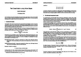
Figure 1 shows the general scheme of the proposed distribution-based algorithm. As we can observe there are two clearly differentiated steps: learning and sampling. At learning time a probability distribution for each pair hterm,class statei is learnt from the unmodified training set (corresponding to the current split of the validation) projected over the term and the class (Dh↓ti ,C ). Then, at sampling time all the distributions learnt for a class state 3

Notice that a full instance contains the frequency fi of term ti in the sampled document plus the class the document (e-mail) belongs to.

9

are used to build (by sampling the corresponding one for each term in turn) each one of the b desired documents for such a class state. This sampling process is repeated for all the class states in order to get a balanced artificial training set. In

Dh training set, C class variable |V | = r the number of terms/features, b #new instances to sample per class,

Out

newDh whole new and fully balanced training set /* learning phase */

1 2 3

for each class ck ∈ C do for each term/feature ti , i = 1, . . . , r do learn probability distribution Pik from Dh↓ti ,C /* sampling phase */

4

newDh ← ∅

5

for each class ck ∈ C do

6

for p=1 to b do

7

newDoc = new double[r+1]

8

for each term/feature ti , i = 1, . . . , r do

9

newDoc[i] = sample value from Pik

10

newDoc[r+1]=ck //add class label

11

newDh = newDh ∪ newDoc

12

return newDh Fig. 1. Distribution-based balancing algorithm.

Of course there are some degrees of freedom in the previous algorithm: the number of documents to be sampled for each class and (mainly) the kind of probability distribution used to model the training set. In this paper, we experiment with four different probability distributions: Uniform, Gaussian, Poisson and Multinomial. • Uniform Distribution. There are several works in the literature (e.g. [15]) which, using binomial classes, conclude that there is not much difference whether sampling by using information extracted from the learning data, or not. Sampling (almost) without using information about the training set can be modeled by learning a uniform distribution. In this way the only information we collect is the max value found for term ti restricted to those samples belonging to class ck . Later, in the sampling process we simply generate a uniform number in the interval [0, maxki ]. We will use 10

this distribution as a baseline threshold to analyze the advantages of the more informed ones. • Gaussian Distribution. The Gaussian distribution is the most frequently used distribution in statistics and computer science due to its natural capacity for correctly approximating models. In our case it is specially appropriate when the relation class-term represents a single concept because of its uni-modal nature. In the univariate Gaussian distribution we assume the frequency fj of term ti conditioned to class state ck as follows: (fj − µ)2 1 . f (ti = fj ) = √ exp − 2σ 2 σ 2π "

#

Thus, learning a univariate Gaussian Distribution consists simply of computing the mean and standard deviation of frequencies for term ti from data restricted to class state ck . Sampling from a Gaussian distribution can be done, for example, following the well known Box and Muller method (see for example [36], chapter 2). It should be pointed out that whenever the sampled value is less than 0, we set it to 0 since we are working with frequencies and negative values make no sense. • Poisson Distribution. As pointed out in [21] “if we think that the occurrence of each term is a random occurrence in a fixed unit of space (i.e. a length of document), then the Poisson distribution is intuitively suitable to model the term frequencies in a given document”. Because of this, the Poisson model has been investigated in the information retrieval community and applied to text classification [21]. Thus, we think that it is a good alternative to be considered for distribution modeling in our balancing algorithm. In the Poisson distribution we assume the frequency fj of term ti as follows: P (ti = fj ) =

e−λ λfj fj !

(4)

where λ is the Poisson mean. Therefore the learning step is simply a matter of computing λ of term ti restricted to class state ck . Sampling from a Poisson distribution is also a well-known process (see for example [36], chapter 2). • Multinomial Distribution. Following the generative distribution from the Naive Bayes Multinomial Model [20] described in formula 2, and once we have learnt the term distribution by class following expression 3, we are ready to generate as many documents as the parameter b indicates. In this case the P (|di |) distribution is assumed to follow a Poisson distribution, Equation 4, which is unidimensional and independent of the class. So by the estimation of the parameter λ as the mean number of terms in a 11

document, that is, the mean length of documents, we can simulate the number of terms in a newly-generated document. Once the number of terms is given, we pick the terms in the generated document by simulating the probabilities P (tl |cj ) as many times as the number of terms has been indicated by the Poisson distribution. So, in the structure of the algorithm shown in Figure 1, the changes are: (1) Values to compute are λ and the probabilities for each term given the class following expression 3. (2) Each term will have the value representing the times that it was drawn following the Multinomial distribution P (tl |cj ) according to the length of document generated following a Poisson distribution.

5

Experiments

In this section we present our experimental study over e-mail foldering using the proposed distribution-based balancing method. We emphasize that our experiment is directly related with e-mail foldering and because of the nature of this problem, perhaps the conclusions here obtained can be extended to similar problems, that is, those having a class variable with large cardinality and numerical variables as predictive attributes. For the sake of completeness, apart from using our approach instantiated with Uniform, Gaussian, Poisson and Multinomial distributions, we also consider the well-known SMOTE algorithm, but slightly modified to deal with multi-class datasets. As classifier we use NBM as it was our aim to improve its performance in the e-mail foldering problem, but for comparison we also use support vector machines and instance-based learning.

5.1

Test suite

As in [3,22], we have used datasets corresponding to seven users from the ENRON corpus (mail from these users and a temporal line in increasing order can be downloaded from http://www.cs.umass.edu/∼ronb). The downloaded data was preprocessed according to the process described in Section 2.2. To do this we coded our own program in Java, and designed it to interact with Lucene information retrieval API 4 and to output a sparse matrix M [numDocs, numTerms] codified as an .arff file, i.e., a file following the input format for the WEKA data mining suite [45]. Table 1 describes the main characteristics of the datasets obtained. The last 4

http://lucene.apache.org/who.html

12

two columns are intended to show the degree of imbalance in the datasets. As in [41], we show (base,peak ), where base is the number of documents of the minority class and peak is the number of documents in the majority class. However, we think this measure is not sufficiently representative of the degree of imbalance because it represents different distributions in the same way, e.g., (1,100) is valid for {1, 100} or {1, 100, 100, 100} or {1, 100, 1, 100, 1, 100}, which clearly represents different degrees of imbalance. Because of this we have added (µ,σ) to the description, µ being the mean of documents per class and σ the standard deviation of the mean. We find σ is a very informative value concerning the imbalance present in the dataset. A clear indication of the degree of imbalance in the problem we are dealing with (e-mail foldering) is that in the seven users (datasets) considered, the standard deviation is greater than the average. Besides this, we also computed the kurtosis degree for each dataset, which in this case represents the degree of concentration of the number of documents per class around the mean number of documents per class. A graphical representation of the imbalance in our datasets is shown in a Box and Whisker plots (Figure 2), where the inputs used were the number of instances per class state. Table 1 Instances, Classes, Attributes, and degree of imbalance in the datasets

5.2

#I

#C

#A.

(base : peak)

(µ ± σ)

Kurtosis

lokay-m

2489

11

18903

(6:1159)

226.3±316.3

2.75

sanders-r

1188

30

14463

(4:420)

39.6±75.6

17.05

beck-s

1971

101

13856

(3:166)

19.5±24.5

13.08

williams-w3

2769

18

10799

(3:1398)

153.8±379.4

4.10

farmer-d

3672

25

18525

(5:1192)

146.9±255.5

7.77

kaminski-v

4477

41

25307

(3:547)

109.2±141.9

1.66

kitchen-l

4015

47

34762

(5:715)

85.4±122.8

11.75

Experimental design

Our goal is to study whether the classifiers, specially NBM, perform better after balancing the datasets. To be more confident in our conclusions, we carry out a statistical analysis in which we compare the results with and without balancing, and we also contrast the results obtained using different classifiers. In the experiments we deal with the following actors: • Balancing algorithms. To balance the training sets we use the proposed method instantiated with the four mentioned distributions: Uniform, Gaussian, Poisson and Multinomial. For comparison, we also consider SMOTE [7]. SMOTE was initially proposed by its author for binomial classes and performs the balancing by sampling synthetic documents from a minority class in a given percentage, and then randomly under-sampling as many 13

Fig. 2. Graphical representation of the imbalance degree in the seven e-mail users.

majority class documents as desired. To apply SMOTE in a multi-class problem, we select the number (b) of documents to re-sample for each class and apply SMOTE to over-sample, without replacement (the SMOTE algorithm does not perform replacement), all classes with cardinality lower than b until obtaining b documents for those classes; then, for classes with cardinality over b, we randomly remove as many documents as necessary to get cardinality b. • Document representation. Documents have been represented by using frequencies and tf*idf. Computation of tf*idf is done incrementally, that is, trying to reproduce the fact that we have a dynamic problem and not a static one, where tf*idf can be computed at the beginning by using all the available information. In our case the classifier should categorize incoming e-mails as they are downloaded into the user inbox folder. So, when testing using our evaluation methodology, test e-mail i should be represented with a tf*idf value where the idf part is computed using the training set and test e-mails from 0 to i − 1, instead of using all s test documents, since documents i + 1 to s are not supposed to be in the inbox folder yet. In this way, incremental time-based split validation needs more time but is more realistic. When balancing is carried out by learning any of the distributions presented in Section 4, the parameters needed (max, µ, σ, λ) are computed using frequency representation, and then the new training set is sampled still using frequencies representation. Thus, tf*idf conversions are performed later when training and testing the classifier. • Classifiers. We have used three different classifiers that are commonly considered when dealing with text categorization problems: Naive Bayes Multinomial (NBM) [31], Support Vector Machine (SVM) [4] and k -Nearest Neigh14

bors (k -NN) [11]. For NBM we used the implementation provided in the WEKA API. For SVM, we used the implementation available in WLSVM [10], which can be viewed as an implementation of the LibSVM [6] running under WEKA environment. For k -NN, we implemented our own code by using WEKA API. Different values of k were tested and two distance metrics: Euclidean and Cosine distances. In this paper we only show the results for the best configuration found: k =15 and the Cosine distance which is also the standard similarity metric in text, and it is computed by: Pn #» fiu × fiv u · #» v q sim(u, v) = #» = P i=1 Pn n | u | × | #» v| 2 2 i=1 fiu × i=1 fiv

Where n is the number of dimensions (attributes) of each vector and fiu the value of dimension i in vector (document) u. Having the previous setting in mind, we ran three different experiments: Experiment 1.- To compute the baseline against which to compare, we ran an incremental time-based split evaluation (see Section 2.2) on each user in Table 1 without balancing. With respect to the value of s in the time-based split evaluation, in all the experiments carried out in this paper we have used the value recommended in Bekkerman’s work, that is, the number (s) of emails to classify in each split is 100. We ran the three mentioned classifiers for both types of document representation: frequencies and tf*idf. SVM performed statistically the same in both cases so from now on we only show its results for tf*idf, which is the configuration suggested in the literature. For k-NN, we only show results for tf*idf because that is the configuration which finally obtains the best results. Finally, because NBM is the main classifier under study in this paper we show results for both representations: frequencies and tf*idf. The results are shown in Table 2, where each entry represent the accuracy averaged over all the folds tested in the time-split validation process. Table 2 Baseline accuracy for 7 e-mail users. NBM freq

NBM tfidf

SVM tfidf

k-NN tfidf

lokay-m

75.27

63.65

79.12

39.54

sanders-r

55.51

48.90

66.20

35.97

beck-s

28.26

17.60

36.87

9.00

williams-w3

91.69

88.87

90.52

86.06

farmer-d

69.64

55.34

73.98

37.63

kaminski-v

45.61

34.75

54.26

9.92

kitchen-l

32.19

34.44

51.10

14.28

Mean

56.88

49.08

64.58

33.20

Experiment 2.- In this experiment we test the behaviour of our proposal, that is, instead of learning the classifiers from the original dataset, we learn them 15

from the artificially balanced dataset. Because of the randomness introduced by the sampling process, we run each balancing algorithm five times and show averaged results. In all the cases the number of documents b to sample per class is set to 30. Tables 3 and 4 show the results obtained. Each entry in the tables represents the accuracy averaged over all the folds tested in the timesplit validation and coming from the five independent executions. Comparison between baseline algorithms (Table 2) and balancing algorithms was done by using a Wilcoxon signed rank test [43,9] (α=0.05), taking as input the timesplit values from the corresponding user-classifier. When the balanced userclassifier is found to be statistically better than the baseline (not balanced), a • is placed inside its corresponding cell. Table 3 Results when balancing with the SMOTE algorithm. NBM freq

NBM tfidf

SVM tfidf

k-NN tfidf

lokay-m

67.94

•67.72

68.82

•57.79

sanders-r

•72.21

•73.28

59.59

•69.82

beck-s

•45.41

•45.49

•42.80

•39.86

williams-w3

87.20

74.43

87.75

64.84

farmer-d

61.21

44.70

72.77

37.15

kaminski-v

43.22

•42.42

49.65

•34.85

kitchen-l

35.92

•38.54

49.72

•32.68

Mean

59.02

55.23

61.59

48.14

In Table 5 we show a paired comparison between each two kinds of balancing methods over the four classification methods used (NBM freq, NBM tdidf, SVM tfidf and k-NN tfidf). Comparison is in the form x − y − z, where x stands for #beats, y stands for #ties and z stands for #loses. For example, in the first cell, the comparison 15-5-8 means that the SMOTE method performed statistically better than the Uniform Distribution method 15 times, statistically the same 5 times and has performed statistically worse 8 times. Experiment 3.- Finally we studied the effect of b on the performance of the distribution-based balancing algorithms. We focus on a representative case as is the case of using the Gaussian distribution for balancing, the NBM classifier and tf*idf document representation. We run this configuration using values for b from 10 to 60, and the results are shown in Figure 3.

5.3

Discussion of Results

Experiment 1: baseline. Table 2 shows the results obtained after performing time-based split evaluation on seven users from the Enron Corpus without preprocessing that instances set. Results show, as in [3], that SVM-tfidf outperforms by far other common classifiers such as NBM. Users with worst 16

Table 4 Results when balancing with the proposed distribution-based algorithm. NBM freq

NBM tfidf

SVM tfidf

k-nn tfidf

lokay-m

52.02

59.20

36.70

49.24

sanders-r

59.33

68.78

71.99

66.60

beck-s

•43.32

•48.76

39.93

•43.13

williams-w3

63.56

66.44

46.42

38.81

farmer-d

52.05

51.38

35.29

•46.31

kaminski-v

40.69

•51.80

28.72

•49.52

kitchen-l

33.11

•42.05

26.11

•37.18

Mean

49.15

55.48

40.74

47.26

(a) Uniform Distribution lokay-m

70.77

•71.51

47.58

•55.95

sanders-r

72.39

•75.23

74.79

•76.02

beck-s

•45.88

•50.55

•44.33

•45.00

williams-w3

84.27

80.78

81.50

77.22

farmer-d

67.11

•64.15

65.93

•54.41

kaminski-v

•52.02

•56.68

55.39

•52.20

kitchen-l

•38.72

•46.45

37.24

•34.66

Mean

61.59

63.62

58.11

56.49

(b) Gaussian Distribution lokay-m

70.68

•73.20

69.95

•60.35

sanders-r

•75.40

•75.88

57.09

•74.09

beck-s

•45.17

•48.53

41.17

•44.05

williams-w3

88.93

77.96

85.62

66.65

farmer-d

65.87

55.25

68.28

•48.72

kaminski-v

46.54

•49.36

45.67

•45.07

kitchen-l

•37.10

•41.92

39.95

•38.44

Mean

61.39

60.30

58.25

53.91

(c) Poisson Distribution lokay-m

70.01

•72.41

67.94

•61.25

sanders-r

74.97

•74.84

55.30

•71.66

beck-s

•45.09

•49.33

40.48

•46.19

williams-w3

89.03

78.86

85.47

66.72

farmer-d

63.22

54.49

70.25

•47.55

kaminski-v

44.48

•47.49

46.10

•42.34

kitchen-l

•35.84

•41.57

40.00

•37.34

Mean

60.38

59.86

57.93

53.29

(d) Multinomial Distribution

results are those with a lower σ value in Table 1, which also corresponds with the higher cardinality of class. Thus, we find in this dataset that high class cardinality leads to low standard deviation in the number of documents per class, and this is an indicator of classifiers’ performance on such databases. We also find that Williams gets a very high performance so it is not an easy 17

Table 5 Paired comparison between balancing methods. SMOTE Uniform

Uniform

Gaussian

Poisson

Multinomial

15-5-8

6-7-15

4-7-17

4-11-13

2-3-23

3-8-17

3-10-15

13-11-4

14-10-4

Gaussian Poisson

10-16-2

Fig. 3. Different values for b using NBM and tf*idf docs. representation.

target to improve.

Experiment 2: balancing In Table 3 we present the results obtained when balancing training sets using the SMOTE method, and in Table 4 we show results for our proposed distribution-based balancing methods. In both tables we include a • symbol when the algorithm associated to a cell performs statistically better than its corresponding cell in the baseline in Table 2. Finally, a pairwise comparison between balancing methods is presented in Table 5. SMOTE balancing proves to be a good choice for preprocessing skewed datasets. Its results outperform the baseline for some users, specially for NBM-tfidf and k-NN-tfidf classifier configuration. On the other hand, SVM only gets statistical improvement in one user and it even decreases in some others. Our distribution-based methods can be classified as one random (Uniform) and three directed (Gaussian, Poisson and Multinomial). Results for Uniform resampling are the worst although several statistical improvements are achieved. Comparing Gaussian, Poisson and Multinomial re-samplings by looking at Table 5 we can conclude that a reasonable order from best to worst could be: Gaussian > P oisson > M ultinomial > U nif orm. In particular, the best choice seems to be Gaussian balancing with the NBM classifier and tf*idf representation. Furthermore, as happens when using SMOTE, the SVM classifier does not get real improvement after balancing, thus indicating that SVM is strong in imbalanced situations, so performing re-sampling, at least in the case of using our methods and SMOTE, does not provide any improvement 18

and even worsens the learning stage. This corroborates a study by [17] which concludes that SVM is robust against imbalanced datasets. Finally, comparing random and directed re-sampling, we find support for our hypothesis which expected that directed balancing alleviates the overlapping problem. Moreover, this provides evidence to suggest that imbalance is not the only problem in skewed datasets. When comparing SMOTE against our proposed distribution-based methods in Table 5, we find that SMOTE performs better than our random distributionbased method, but worse than our three suggestions for directed distributionbased methods. We clearly conclude that our proposal (except for Uniform distribution) outperforms SMOTE at least when applied to text categorization with more than 2 classes. With respect to document representation, if we focus on NBM, whose results are shown with frequencies and tf*idf documents representation, we can see that in the baseline NBM with frequencies performs better than NBM with tf*idf but, after balancing the data, NBM with tf*idf performs considerably better and achieves statistically the same results as NBM with frequencies; thus, we interpret this as proof that tf*idf representation is more imbalancedsensitive than frequency representation. Comparing users by looking at Table 1, Figure 2 and Table 4, we find that users which usually obtain statistical improvement are: beck-s, kaminski-v, kitchen-l and sanders-r. These four users are those with a larger cardinality for their class attribute and which present lower outliers in their box and whisker plot. Furthermore, with respect to their (µ, σ) representation, they are also the user with lowest µ and σ values; respect to kurtosis degree, higher values clearly point to a higher need of balancing. Thus, based on these results, we suggest that a good way to predict performance improvement after balancing a dataset may be one of these: (1) cardinality class, (2) outliers in box and whisker plot, (3) low (µ, σ) values and/or (4) high kurtosis values . For example, by looking at Table 1 we could predict that a good order of datasets with a greater need for a balancing process are (from more to less): beck-s, sanders-r, kitchen-l, kaminski-v, farmer-d, lokay-m and williams-w3. We suggest using the kurtosis value since this is just a single value and very related to the balancing need.

Experiment 3: number b of documents per class. We ran the configuration Gaussian Distribution with classifier NBM and tf*idf representation using values for b from 10 to 60, and the results are shown in Figure 3. Choosing the value for b should not only be based on performance but also on the computational cost of sampling b new instances for each class. Thus, based on Figure 3, we suggest using values from 30 to 40, since the computational cost is quite high from 30 documents and above, while the improvement acheived is not significant. 19

6

Conclusions

For the NBM classifier, we achieved our goal of improving its performance in the e-mail foldering task, which is of great interest given that NBM is a well-known standard for text classification. We have presented a comparison of four kinds of distributions (one random and three directed) to fully re-sample training datasets for multi-class classification, applied to e-mail categorization; we have also compared our results with the well known SMOTE balancing method. The results support our main hypothesis, which stated that a directed re-sampling method not only balances the training set but also reduces the problem of overlapping among classes, while random re-sampling is only capable of dealing with the imbalance problem. Furthermore, we have found evidence that the SVM classifier is very robust under imbalanced conditions, so its performance does not improve after balancing. Comparing with SMOTE, we find that our distribution-based methods statistically outperform it, except for the Uniform distribution. Finally, we found a strong correlation between datasets which usually perform better after balancing; that is, it can be expected that datasets whose performance improves after balancing will be those which present a large cardinality class, low outliers in a box and whisker plot, low (µ, σ) values and/o high kurtosis degree.

References

[1] N. Abe, An iterative method for multi-class cost-sensitive learning, in: In Proceedings of the Tenth ACM SIGKDD International Conference on Knowledge Discovery and Data Mining, 2004, pp. 3–11. [2] R. Bekkerman, K. Eguchi, J. Allan, Unsupervised non-topical classification of documents, Tech. rep., Center of Intelligent Information Retrieval, Massachusetts Univ. (2006). [3] R. Bekkerman, A. McCallum, G. Huang, Automatic categorization of email into folders: Bechmark experiments on enron and sri corpora, Tech. rep., Department of Computer Science. University of Massachusetts, Amherst. (2005). [4] B. E. Boser, I. M. Guyon, V. N. Vapnik, A training algorithm for optimal margin classifiers, in: Proceedings of the 5th Annual ACM Workshop on Computational Learning Theory, ACM Press, 1992, pp. 144–152. [5] P. K. Chan, S. J. Stolfo, Toward scalable learning with non-uniform class and cost distributions: A case study in credit card fraud detection, in: In Proceedings of the Fourth International Conference on Knowledge Discovery and Data Mining, AAAI Press, 1998, pp. 164–168.

20

[6] C. Chang, C. Lin, LIBSVM: a library for support vector machines, software available at www.csie.ntu.edu.tw/∼cjlin/libsvm (2001). [7] N. V. Chawla, K. W. Bowyer, W. P. Kegelmeyer, SMOTE: Synthetic minority over-sampling technique, Journal of Artificial Intelligence Research 16 (2002) 321–357. [8] N. V. Chawla, N. Japkowicz, A. Kotcz, Editorial: special issue on learning from imbalanced data sets, SIGKDD Explorations Newsletter 6 (1) (2004) 1–6. [9] J. Demsar, Statistical comparisons of classifiers over multiple data sets, Journal of Machine Learning Research 7 (2006) 1–30. [10] Y. El-Manzalawy, V. Honavar, WLSVM: Integrating LibSVM into Weka Environment, software available at www.cs.iastate.edu/∼yasser/wlsvm (2005). [11] E. Fix, J. L. Hodges, Discriminatory analysis, nonparametric discrimination, Tech. rep., USAF scholl of Aviation Medicine, Randof field, Project 21-49-004, Rept 4 (1951). [12] G. Forman, An extensive empirical study of feature selection metrics for text classification, Journal of Machine Learning Research 3 (2003) 1289–1305. [13] I. Guyon, A. Elisseeff, An introduction to variable and feature selection, Journal of Machine Learning Research 3 (2003) 1157–1182. [14] Y.-J. Hu, Constructive induction: covering attribute spectrum. In Feature Extraction, Construction and Selection: a data mining perspective, Kluwer, 1998. [15] N. Japkowicz, The class imbalance problem: Significance and strategies, in: In Proceedings of the 2000 International Conference on Artificial Intelligence (ICAI), 2000, pp. 111–117. [16] N. Japkowicz, Concept-learning in the presence of between-class and withinclass imbalances, in: AI ’01: Proceedings of the 14th Biennial Conference of the Canadian Society on Computational Studies of Intelligence, Springer-Verlag, London, UK, 2001, pp. 67–77. [17] N. Japkowicz, S. Shaju, The class imbalance problem: A systematic study, Intelligent Data Analysis 6 (5) (2002) 429–449. [18] T. Jo, N. Japkowicz, Class imbalances versus small disjuncts, SIGKDD Explorations Newsletter 6 (1) (2004) 40–49. [19] T. Joachims, Learning to classify text using support vector machines, Kluwer Academic Publishers, 2002. [20] S.-B. Kim, K.-S. Han, H.-C. Rim, S. H. Myaeng, Some effective techniques for naive bayes text classification, IEEE Transactions on Knowledge and Data Engineering 18 (11) (2006) 1457–1466.

21

[21] S.-B. Kim, H.-C. Seo, H.-C. Rim, Poisson naive bayes for text classification with feature weighting, in: Proceedings of the sixth international workshop on Information retrieval with Asian languages, 2003, pp. 33–40. [22] B. Klimt, Y. Yang, The ENRON corpus: a new dataset for email classification research, in: 15th European Conference on Machine Learning, 2004, pp. 217– 226. [23] M. Kubat, S. Matwin, Addressing the curse of imbalanced training sets: onesided selection, in: In Proceedings of the Fourteenth International Conference on Machine Learning, Morgan Kaufmann, 1997, pp. 179–186. [24] O. Larsen, A. Freitas, J. Nievola, Constructing x-of-n attributes with a genetic algorithm, in: Proc Genetic and Evolutionary Computation Conf (GECCO2002), 2002. [25] D. Lewis, Representation and learning in information retrieval, Ph.D. thesis, Department of Computer Science, University of Massachusetts (1992). [26] D. Lewis, Naive (Bayes) at forty: The independence assumption in information retrieval., in: Proceedings of ECML-98, 10th European Conference on Machine Learning, 1998, pp. 4–15. [27] Y. Lin, Y. Lin, Y. Lee, Y. Lee, G. Wahba, G. Wahba, Support vector machines for classification in nonstandard situations, in: Machine Learning, 2002, pp. 191–202. [28] H. Liu, H. Motoda, Feature Extraction Construction and Selection: a data mining perspective, Kluwer Academic Publishers, 1998. [29] Y. Liu, H. T. Loh, A. Sun, Imbalanced text classification: A term weighting approach, Expert Systems with Applications 36 (1) (2009) 690–701. [30] L. Malazizi, D. Neagu, Q. Chaudhry, Improving imbalanced multidimensional dataset learner performance with artificial data generation: Density-based classboost algorithm., in: P. Perner (ed.), ICDM, vol. 5077 of LNCS, Springer, 2008, pp. 165–176. [31] A. McCallum, K. Nigam, A comparison of event models for naive bayes text classification, in: AAAI/ICML-98 Workshop on Learning for Text Categorization, 1998, pp. 41–48. [32] V. Mitra, C.-J. Wang, S. Banerjee, Text classification: A least square support vector machine approach, Applied Soft Computing 7 (3) (2007) 908–914. [33] E. Monta˜ n´es, E. F. Combarro, I. D´ıaz, J. Ranilla, Towards automatic and optimal filtering levels for feature selection in text categorization, in: Proceedings of the 6th International Symposium on Intelligent Data Analysis (IDA’05), 2005, pp. 239–248. [34] R. C. Prati, G. Bastista, M. C. Monard, Class imbalances versus class overlapping: an analysis of a learning system behavior, in: MICAI, LNAI, 2004, pp. 312–321.

22

[35] B. Raskutti, A. Kowalczyk, Extreme re-balancing for SVMs: a case study, SIGKDD Explorations Newsletter 6 (1) (2004) 60–69. [36] R. Y. Rubinstein, B. Melamed, Modern Simulation and Modeling (Wiley Series in Probability and Statistics), Wiley-Interscience, 1998. [37] M. Sahami, S. Dumais, D. Heckerman, E. Horvitz, A bayesian approach to filtering junk e-mail, in: Learning for Text Categorization: Papers from the 1998 Workshop, AAAI Technical Report WS-98-05, 1998. [38] S. Sakurai, A. Suyama, An e-mail analysis method based on text mining techniques, Applied Soft Computing 6 (1) (2005) 62–71. [39] G. Salton, C. Buckley, Term weighting approaches in automatic text retrieval, Tech. rep., Cornell University (1987). [40] S. Scott, S. Matwin, Feature engineering for text classification, in: Proceedings of ICML-99, 16th International Conference on Machine Learning, 1999, pp. 379–388. [41] E. Stamatatos, Author identification: Using text sampling to handle the class imbalance problem, Information Processing & Management 44 (2) (2008) 790– 799. [42] G. M. Weiss, Mining with rarity: a unifying framework, SIGKDD Explorations Newsletter 6 (1) (2004) 7–19. [43] F. Wilcoxon, Individual comparisons by ranking methods, Biometrics Bulletin 1 (6) (1945) 80–83. [44] I. H. Witten, Z. Bray, M. Mahoui, W. J. Teahan, Text mining: A new frontier for lossless compression, in: Proceedings of Data Compression Conference, 1999, pp. 198–207. [45] I. H. Witten, E. Frank, Data Mining: Practical Machine Learning Tools and Techniques (Second Edition), Morgan Kaufmann, 2005. [46] Z. Zheng, X. Wu, R. K. Srihari, Feature selection for text categorization on imbalanced data, SIGKDD Explorations Newsletter 6 (1) (2004) 80–89. [47] Z.-H. Zhou, X.-Y. Liu, On multi-class cost-sensitive learning, in: AAAI, 2006.

23