IMPROVING THE PERFORMANCE OF PARTICLE SWARM OPTIMIZATION USING ADAPTIVE CRITICS DESIGNS Sheetal Doctor and Ganesh K. Venayagamoorthy Real-Time Power and Intelligent Systems Laboratory Department of Electrical and Computer Engineering University of Missouri – Rolla, MO 65409, USA
[email protected] two benchmark functions, namely the Rastrigrin and the Rosenbrock minimization functions [4].
ABSTRACT Swarm intelligence algorithms are based on natural behaviors. Particle swarm optimization (PSO) is a stochastic search and optimization tool. Changes in the PSO parameters, namely the inertia weight and the cognitive and social acceleration constants, affect the performance of the search process. This paper presents a novel method to dynamically change the values of these parameters during the search. Adaptive critic design (ACD) has been applied for dynamically changing the values of the PSO parameters.
Sections 2 and 3 give a brief description of PSO and ACDs respectively. Section 4 describes the Dynamic PSO (DPSO) and section 5 presents some results for two benchmark functions. Finally, the conclusions and future work is given in Section 6. 2. PARTICLE SWARM OPTIMIZATION PSO is also a population based search strategy. A problem space is initialized with a population of random solutions in which it searches for the optimum over a number of generations/iterations and reproduction is based on prior generations. The concept of PSO is that each particle randomly searches through the problem space by updating itself with its own memory and the social information gathered from other particles [5].
1. INTRODUCTION Particle Swarm is a swarm intelligence based algorithm developed by James Kennedy and Russell Eberhart in 1995 [1]. This algorithm is modeled on the behavior of a school of fish / flock of birds. PSO has also been used in a variety of applications including generator maintenance scheduling, electromagnetics [2].
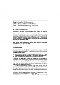
Figure 1 gives the vector representation of the PSO search space. In figure 1, Vpd and Vld represent the effect of ‘Pbest’ and ‘Gbest’ on the individual. The basic PSO velocity and position update equations are given by (1) and (2) respectively.
PSO is a powerful optimization tool. It is a stochastic algorithm and the PSO operation itself is complicated and difficult to understand. The performance of a PSO based search can be changed by varying the values of the PSO parameters, inertia weight ‘w’, cognitive and social acceleration constants ‘c1’ and ‘c2’ respectively, thereby giving it the flexibility to optimize its own performance. The dynamics of many systems change with time and therefore it may be difficult to find one set of the PSO parameters which are optimum over the entire range of operation.
Y T
Vnew Pold
Approximate Dynamic Programming (ADP) is a concept that tries to find optimum solutions to problems where a method to find the exact solutions is difficult. ADP approximates an optimal solution to a problem based on a utility function. Adaptive Critics Design (ACD) is an optimization tool used to carry out ADP. It combines the concepts of dynamic programming and reinforcement learning [3]. ACD has been applied in this paper for dynamically changing the value of the PSO parameters (DPSO), w, c1 and c2. The technique has been applied to
0-7803-8916-6/05/$20.00 ©2005 IEEE
Pnew
Vold
Vld Vpd X
Figure 1. Vector representation of PSO (T is the target)
Vnew = w × Vold + c1 × rand × ( Pbest − Pold ) + c 2 × rand × (Gbest − Pold ) Pnew = Pold + Vnew
1
(1)
(2)
Where, Vnew Vold Pnew Pold w c1 & c2 rand
New velocity calculated for each particle Velocity of the particle from the previous iteration New position calculated for each particle Position of the particle from the previous iteration Inertia weight constant Cognitive and social acceleration constants Generates a random value in the range [0 1]
PSO based application
TDL
Gfit(k)
A(k-1) Gfit(k) TDL
Action Network
A(k)
TDL
Critic Network
Gfit(k)
J(k)
TDL
3. ADAPTIVE CRITICS DESIGNS
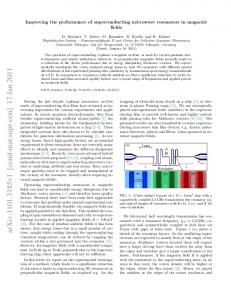
Figure 2. Block diagram of DPSO
Adaptive critic designs are used to determine the optimal control law for a dynamic process [3]. ACDs are used to approximate the Bellman’s equation of dynamic programming, the cost-to-go function given by (3), where γ is a discount factor and is in the range [0,1]. The objective of ACDs is to develop an optimal control strategy.
As seen in figure 2, Gfit, a function of the fitness value of the PSO process, is taken as the input to the action and critic networks. The action network gives out the values of the PSO parameters w, c1 and c2 which drive the application. These values are also fed to the critic network. The output of the action network is given by (4)
∞
J ( x (k )) = ∑ γ k (U ( x(k )) )
A ( k ) = w ( k ) , c1 ( k ) , c2 ( k )
(3)
(4)
k =0
A. Training the Critic Network
U(k) is called the utility function. The utility function is custom to the application and is chosen by the designer and it embodies the design requirements of the system.
Figure 3 shows the block diagram for the training of the critic network. The critic network is initially trained without the action network. The critic network can be trained for different values of the w, c1 and c2. They can be constants, linearly increasing or decreasing or randomly generated. w is generated in the range [0.2, 1.2] and, c1 and c2 are generated in the range [0.4, 2]. These inputs are fed to both the PSO application as well as the critic network. The error signal generated at the output is backpropagated and the weights of the critic network are updated.
ACDs adapt two neural networks successively to learn the dynamics of the process. These are namely the Action Neural Network, which provides the control signal for the process and the Critic Neural Network which evaluates the performance of the action network or approximates the Bellman’s equation. The action network dispenses a control signal in order to optimize (minimize or maximize) the output of the critic. The action network may learn this control signal through a model network or directly through the critic’s performance. Thus, the two neural networks together learn the system dynamics and are able to achieve an optimal control law for the process dynamically. The initialization of the weights of the neural networks does not affect the final results.
w(k)
J(k)
w(k-1) c1(k) c1(k-1) c2(k) c2(k-1)
×
U(k)
Critic Neural Network
Gfit(k)
There are four types of adaptive critic designs [3]. This paper uses the Action Dependent Heuristic Dynamic Programming (ADHDP) structure.
γ
Target γ*J(k) + U(k)
Gfit(k-1) 1 w(k-1) w(k-2) c1(k-1)
4. DYNAMIC PARTICLE SWARM OPTIMIZATION
c1(k-2) c2(k-1) c2(k-2)
The action and the critic network need to be trained for the problem at hand before the DPSO can be applied directly to the problem. Figure 2 shows the block diagram for DPSO.
+
J(k-1) Critic Neural Network
-
∑ Ec
Gfit(k-1) Gfit(k-2) 1
Figure 3. Block diagram for the critic training
2
Equation (5) gives the error value for which the critic network is trained. Equation (6) gives the value of the utility function. The critic network needs to be trained for a number of runs of the PSO applications. The fitness function of the PSO application is fed to the critic network in order to tune the network for the application at hand. This training is carried out till the output of the critic follows the target as closely as possible.
Ec = γ × J ( k ) + U ( k ) − J ( k − 1)
5. DPSO FOR BENCHMARK FUNCTIONS DPSO is applied to the Rastrigrin and Rosenbrock [4] minimization functions given by (7) and (8) respectively, where ‘N’ is the number of dimensions of the function. The PSO population is initialized for a dimension of 10 and a population size is 20. The population is initialized in the asymmetric initialization range of [2.56, 5.12] and [15, 30] for the Rastrigrin and Rosenbrock functions respectively [4]. The utility function for both the functions is given by (7) and (8).
(5)
N
U (k ) =
f
(G ( k ))
f rast ( x ) = ∑ ( xi2 − 100cos ( 2π xi ) + 10 )
(6)
fit
i =1 N
i =1
The action network provides the control action for the PSO based system. This value is given as the input to the critic network instead of the random values of w, c1 and c2 as described above. The critic responds to this signal by generating the output J function. The action network is trained such that the output of the critic is minimized. Thus, the outputs of the action network will eventually drive the system efficiently. Figure 4 shows the block diagram for the training of the action network.
PSO based application
PRBS
TDL
Action Neural Network
Gfit(k) TDL
2
)
(8)
(9)
The Tables 1 and 2 show the drastic reduction in the number of iterations required to find the minimum error for both the functions. Figures 5 and 6 show the outputs of the action network during the testing of the ADHDP for the Rastrigrin and Rosenbrock functions. All the results shown in the tables have been averaged over 50 trials. The results shown here have been obtained on 2.2 GHz, Pentium 4 processor.
Gfit(k)
TABLE 1. RESULTS FOR RASTRIGRIN FUNCTION Method Previously published [4] PSO (constant w) PSO (linearly decreasing w) Dynamic PSO
A(k) J(k)
TDL
2
U ( k ) = 0.1× G fit ( k )
A(k-1) Gfit(k)
(
f rosen ( x ) = ∑ 100 ( xi +1 − xi2 ) + ( xi − 1)
B. Training the Action Network
(7)
Critic Neural Network
∂J/ ∂A
Error 5.5572 4.2134 0.5258 0
Iterations 1000 819.53 333.85 5.98
TABLE 2. RESULTS FOR ROSENBROCK FUNCTION Method Previously published [4] PSO (constant w) PSO (linearly decreasing w) Dynamic PSO
Figure 4. Block diagram of the action network training The action too can be trained for the different inputs. Figure 4 shows two different sets of inputs. One set gives random values of w, c1 and c2 and the other set is the output of the action network itself. The action network is trained with an error signal taken from the critic network. This is given by ∂J ∂A , where ‘A’ is the output of the action network. The methods for training described above are generic and variations can be incorporated in them for different applications.
3
Error 96.1715 12.7758 10.4645 0.3726
Iterations 1000 811 371.74 369.08
output A of the Action Network
3.5
[2]
G. Ciuprina, D. Ioan, I. Munteanu, “Use Of Intelligent-Particle Swarm Optimization In Electromagnetics”, IEEE Transactions on Magnetics, vol. 38, Issue: 2, pp: 1037 – 1040, March 2002.
[3]
G.K. Venayagamoorthy, R.G. Harley RG, D.C. Wunsch DC, “Applications of Approximate Dynamic Programming in Power Systems Control”, Handbook of Learning and Approximate Dynamic Programming, Si J.; Barto A.; Powell W.; Wunsch DC. (Eds.), Wiley, ISBN 0-471-66054-X, pp. 479 – 515, July 2004.
[4]
Y Shi and R.C Eberhart, “Empirical Study of Particle Swarm Optimization” Proceedings of Congress on Evolutionary Computation. vol. 3, pp: 1950, 6-9 July 1999.
[5]
A. Engelbrecht, Computational Intelligence- An Introduction, John Wiley & Sons, Ltd, England. ISBN 0-470-84870-7, 2002.
w c1
3
c2 2.5
2
1.5
1
0.5
1
2
3
4
5
6
7
Figure 5. Output of the trained action network for Rastrigrin function output A of the Action Network
4.5
w c1 c2
4 3.5 3 2.5 2 1.5 1 0.5
0
10
20
30
40
50
60
70
80
Figure 6. Output of the trained action network for Rosenbrock function 6. CONCLUSION This paper has presented the successfully application of the concepts of approximate dynamic programming to PSO process. The DPSO algorithm drastically improves the performance of the PSO search compared to other approached in literature. Future work can involve exploring other ACD techniques such as DHP or GDHP, for solving these problems. The work considered here assumes that the three PSO parameters are coupled. Future work can also involve optimizing these parameters independently of each other. 7. ACKNOWLEDGMENT The support from the National Science Foundation, USA CAREER grant number: ECS # 0348221 is gratefully acknowledged for this work by the authors. 8. REFERENCES [1]
J. Kennedy and R. Eberhart., “Swarm Intelligence”, Morgan Kauffman Publishers, San Francisco, CA, 2001,. ISBN 1-55860-595-9.
4