In-duct Beamforming Noise Source Estimation and ...

In-duct Beamforming Noise Source Estimation and Mode Detection at the University of S˜ ao Paulo Fan Rig Luciano C. Caldas∗

Rafael G. Cuenca

Escola Polit´ecnica - USP

†

Rudner Lauterjung Q.

EESC - USP

‡

Embraer S/A

Luiz A. Baccal´a Escola Polit´ecnica - USP

An in-duct modal analysis and beamforming technique was used for locating and quantifying noise of a fan rig constructed at University of S˜ ao Paulo (USP). The in-house beamforming software developed has steering vectors derived from duct mode signal representation whose use was illustrated using data obtained from the rig’s 77-microphone duct wall array. Software validation using simulated point spread function map and artificial noise data from NASA-Glenn ANCF rig are shown. Fan rig modes were computed from the 1st to the 4th BPF at the maximum speed of 4250 RPM and 0.1 Mach flow followed by conventional beamforming for different speeds and frequencies that estimate the static noise coming from rotor-stator interaction. Noise coming from the blade-tip and root region were clearly distinguishable in these maps.

Nomenclature BP F P SF b N ~g ~ w C J ψ a Ω k γ, κ j

Blade passing frequency Point spread function Conventional Beamforming map Number of microphones Modal steering vector Normalized steering vector Cross spectral matrix Bessel function of first kind Mode shape function Duct radius Fan speed Wave vector Mode wave number √ Complex number −1

Subscript i Sensor point s Source mesh point j Source point for PSF computation m, n Circumferential and radial mode ∗ Poli-USP,

S˜ ao Paulo, 05508-900, Brazil S˜ ao Carlos, S˜ ao Paulo, 13566-590, Brazil ‡ Embraer, S˜ ao Jos´ e dos Campos, S˜ ao Paulo, Brazil † EESC-USP,

1 of 11 American Institute of Aeronautics and Astronautics

I.

Introduction

The aim of this paper is to describe noise source estimation software developed for use in the newly constructed long-duct low-speed fan rig test facility at the S˜ao Carlos Engineering School from the University of S˜ ao Paulo (USP). The project aims to provide a facility for studying the fluid dynamic details of fan noise generation mechanisms. Consequently the rig was designed for configuration flexibility allowing rig section replacement to suit specific experimental needs. A glimpse of its current configuration can be appreciated in Figure 1. The rig has 0.6m diameter and is 10m long; its basic configuration comprises a 0.5m diameter duct fan stage equipped with a 16-bladed rotor and a 14-vaned stator. The rotor is powered by an 100HP electrical motor fixed by 3 struts allowing experiments up to 4250 RPM and Mach 0.1 flow speed. What sets it apart is its length compared to that of other ducts that operate within anechoic chambers.2, 3, 10 In facilities like this, wall in-duct array of microphones have long been used to measure broadband fan noise.1–3, 10, 11 As such, an array comprising 77-microphones as portrayed in Figure 2(a) was designed. Further details of its geometry can be appreciated in Figure 3 where in the initial microphone array configuration has three separate rings 0.10 and 0.17m apart, each ring comprising 33, 23 and 21 uniformly distributed microphones.

Figure 1: Fan rig constructed in S˜ ao Carlos, Brazil. Left - front view from the bell-mouth; Center Microphone array; Right - 16-Bladed rotor. The acoustic data acquisition system comprises flush-mounted microphones (GRAS 40PH-S2 φ 7mm, bandwidth of 20-20kHz and 50mV /P a average sensitivity) operated via a PXI National Instruments system composed of 5 PXI-4496 boards. Angular motor position is also simultaneously acquired. This paper is organized as follows. Section II provides details of the array processing methods being used in our facility followed by some preliminary processing results (Section III) meant for methodological validation. The paper ends with a brief discussion.

II.

Array Signal Processing Details

An in-house array processing procedures was developed based on the guidelines provided by Lowis1 and Sijtsma11 with the objective of locating not only noise signal sources but also for decomposing data in terms the generated propagating sound modes as described next.

2 of 11 American Institute of Aeronautics and Astronautics

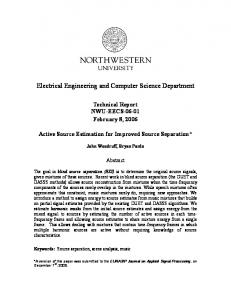
(a) The 3-rings 77-microphones array

(b) 16-bladed fan

Figure 2: Closer look at the acoustic array mount and fan rig.

Figure 3: 77-microphones fan rig array sketch.

A.

Duct-Beamform Imaging

In spatial beamforming imaging and mode detection, microphone pressure values over time, pi , obtained from a duct-array are analysed to infer the distribution and strength of noise sources. Conventional beamforming estimates the spatial pressure density bs at a mesh point ξs by using ~s C w ~s H , bs = w

(1)

~ is the normalized steering where C (N × N ) is the cross-spectral matrix between all microphone pairs and w vector evaluated at the mesh point ξs to all microphones positions ~xi , i.e. ~s = w

~g ||~g||

(2)

where ~g(~x, ~xs , ω) = [g1 (~x1 , ~xs , ω), g2 (~x2 , ~xs , ω), ..., gN (~xN , ~xs , ω)]T

3 of 11 American Institute of Aeronautics and Astronautics

(3)

which, for most beamforming applications, Equation 3 is just the free-field propagation vector. Here one must use an in-duct sound wave propagation vector version that takes into account hard-wall circular duct modes complying with linear uniform flow boundary conditions. At frequency ω, this is given by1 gi (~xi , ~xs , ω) =

j X ψm,n (ri )ψm,n (rs ) j(θi −θs ) −j(zi −zs )γm,n e e 4π m,n Λ2m,n κm,n (ω)

(4)

where Λm,n is a mode normalization factor. Lowis1 and Dougherty4 have recently pointed out that for modes near to cut-off, κ(ω) values approach zero so that produce steering vectors in Equation 4 become dominated by these modes leading to unrealistic beamforming results. To mitigate this effect, Dougherty4 suggests remove κ(ω) from Equation 4. This gives X ψm,n (ri )ψm,n (rs ) ej(θi −θs ) e−j(zi −zs )γm,n (5) gi (~xi , ~xs , ω) = 2 Λ m,n m,n which was the steering vector form adopted in the present work. Note that Equations 4 and 5 are expressed in cylindrical coordinates (r, θ, z) where source location is described xs : (rs , θs , zs ) over mesh where the image is computed, whereas microphone location is denoted by xi : (ri , θi , zi ). Moreover, r ψm,n (r) = Jm (σmn ) (6) a describes the radial and circumferential shape of the (m, n)th mode as function of duct geometry (i.e. a is the duct radius) where Jm (x) is the Bessel function of the first-kind of order m, and σmn is the nth stationary point of order m. Mode wave number equations are given by r −M k − κm,n (ω) σm,n 2 γm,n (ω) = k 2 − (1 − M 2 )( , κ (ω) = ) . (7) m,n 1 − M2 a Real valued κm,n describes cut-on modes whereas complex values characterize cut-off modes that decay exponentially and do not propagate within the duct. B.

Modal analysis

Close inspection of equations 4 and 5 reveals that gi can be re-written in a double sum involving circumferential and radial modes (m, n) XX g= gm,n (8) m

n

(the subscript i was suppressed to simplify notation). Thus beamforming results can be broken into modes:     H H H H g1,0 Cg1,0 g1,0 Cg1,1 · · · g1,0 Cgm,n g1,0  H    H H H g1,1 Cg1,1 · · · g1,1 Cgm,n  g1,1   g1,1 Cg1,0    . Bmodes = [g1,0 g1,1 · · · gm,n ] C  = (9) .. .. .. ..  ..    .  .    . . . H gm,n

H gm,n Cg1,0

H gm,n Cg1,1

···

H gm,n Cgm,n

Mode orthogonality implies that the elements of Bmodes away from the main diagonal are theoretically zero, implying that duct beamforming reduces to a sum of (m, n) independent beamforming maps, one for each singular modal steering vector. Acoustic map mode by mode maps may be computed together with their allied singular mode power at each frequency obtained by integration over each such map.

III.

Results

The two methods were used to validate the beamforming code: (a) use of a synthetically generated point spread function and (b) data from the NASA-Glenn ANCF rig consisting of pure excited modes. After providing illustration under the latter situations, it is presented a sampling of University of S˜ao Paulo fan rig beamforming and modal analysis results. All beamforming map plots use the 20 µP a pressure level reference whereas modal power plots refer to an 1 pW power. 4 of 11 American Institute of Aeronautics and Astronautics

A. 1.

Algorithm Validation Synthetic Point source

The effect of a dipole stationary tonal source, denoted ~j, was simulated following Sijtsma.12 This source induces a CSM given by Cj = ~gjH ~gj = w ~ jH w ~j (10) where w ~ is the steering vector for an unit power source. The beamforming map is obtained by scanning the grid points ξs leading to bjs = w ~ s Cj w ~ sH = w ~ s (w ~ jH w ~ j )w ~ sH = ||w ~ sw ~ jH ||2 (11) which means that the PSF map can be obtained by fixing the steering vector w ~ j at the source position while sweeping w ~ s over the image mesh grid ξs . A simulation result example can be appreciated in Figure 4 for a source located at r = 0.24m, θ = 0 and z = −0.7m. This focal plane (fp), the z distance, is the same of the fan plane. Frequencies in the range between the 1st and 6th BPF equivalent for 4250 RPM were evaluated. It is important to mention that, due to the small number of modes at low frequencies, the source location on the PSF map does not match exactly the desired point ~j and the map has a large main lobe. At 1.13kHz a clearly discernible source close to the wall is event and comprise only 11 cut-on modes. Strong beamforming side-lobes can also be seen. At higher frequencies source discernibility increases followed by diminished side-lobes confirming code plausibility. 2.

Mode detection

Data collected from the NASA-Glenn ANCF6, 7 rig were used to validate the beamforming and modedetection code. Signals were generated using 2 rings of 16 speakers surrounding the duct of the ANCF rig. All parameters combinations were performed for tones at 508Hz and 1016Hz; modes from m=-6 to +6; two fan speeds: idle mode (∼300 RPM) and at ∼1800 RPM. Figures 5 and 6 portray some of these combinations. Together these results confirm the code’s ability to properly capture mode behavior. B.

USP fan rig results

The data for beamforming were acquired at 51.2kHz sample rate with no synchronism system. This was followed by the removal of strong fan tones (BPF) from the broadband noise through a time domain algorithm to estimate and subtract the corresponding sinusoids from the raw signal. After that, data was time resampled producing 512 samples per fan revolution. The cross spectral matrix C between microphones was estimated using Welch’s method, 50% overlapping, Hanning data window of 2048 samples9 . The well-know technique of diagonal removal8 from C was used to remove boundary and shear layer noise from the signals. Beamforming and modal analysis was subsequently performed for frequencies starting from the first to the fourth BPF. Due to the distance from array to the fan stage, (∼0.85m for the closest ring), only cut-on modes are analysed. 1.

Mode analysis at BPF orders

A modal analysis can be appreciated in Figure 7 for 4250 RPM shaft speed obtained by conventional beamforming technique, as described in Section II. The beamforming plots for each mode were integrated over the duct area and the total power was then computed. A dynamic range of 15dB was used both for BPF and mode analysis plots meaning that modes/pressure bellow 15dB of the highest mode/peak are represented as dark plot areas. Modes for BPF in Figure 7 show a strong dominant mode for each order of BPF. Tyler-Sofrin blade-vane modes can be used to understand this observation. For the first BPF, m=-1 and m=-2 are seen. The first relation gives m = 16 − 14 = 2. For 1.5 and 3 BPF strong modes are the same: m=-1 and m=-6. This appears to be a 3rd order relation between blades and vales, just as m = 3 × 16 − 3 × 14 = 6. At 2nd and 4th BPF, modes m=-4 and m=-8 respectively, it is easily explained by m = 2 × 16 − 2 × 14 = 4 and the double of it. The mode m = −1 is not so clear where it comes from. There are 3 struts ∼ 2m away from the rotor/stator supporting the motor. One possible reason for this mode might be a 3-way interaction of rotor, stator and struts, such as: m = 2 × 16 − 2 × 14 − 1 × 3 = 1. 5 of 11 American Institute of Aeronautics and Astronautics

Figure 4: PSF for fan rig configuration with static focused beam using simulation data. Frequencies from 1st to 6th BPF equivalent for 4250 RPM 16-bladed rotor. Source at r = 0.24m and θ = 0.

6 of 11 American Institute of Aeronautics and Astronautics

Figure 5: Modal analysis for data from NASA-Glenn ANCF rig. Beamforming with static beam. Top-left: f=508Hz, mode m=-2. Top-right: f=508Hz, mode m=-3. Bottom-left: f=1.016kHz, mode m=0. Bottomright: f=1.016kHz, mode m=-1. All with fan in idle ∼300 RPM.

Figure 6: Modal analysis for data from NASA-Glenn ANCF rig. Beamforming with static beam. Left: f=1.016kHz, mode m=-5, fan at idle ∼300 RPM. Right: f=1.016kHz, mode m=+4, fan at ∼1800 RPM.

7 of 11 American Institute of Aeronautics and Astronautics

Figure 7: USP fan rig modal analysis. Beamforming with static beam. Top-left: 1 BPF, top-right: 1.5 BPF, mid-left: 2 BPF, mid-right: 2.5 BPF, bottom-left: 3 BPF, bottom-right: 4 BPF. Fan at 4250 RPM.

8 of 11 American Institute of Aeronautics and Astronautics

2.

Beamforming maps

Beamforming plots at multiples of the BPF are not shown in this paper because they do not provide much visual information. However, at some frequencies it is possible to see some interesting results. Figure 8 presents some of these cases for different shaft speed situations. It is worth noting that static beamforming becomes hard if a strong rotating source of noise is placed just ahead of the focal plane. Lowis1 has shown that the capability of the focal beam to distinguish static and rotating source comes from the ‘smearing’ effect, i.e., rotating sources appear smeared in the map when static sources are focused. In other hand, when a rotating-beam is used, the opposite occurs, rotating sources are ‘triggered’ by the beam. In this paper only a static-beam was evaluated leading the appearance of smeared rotating sources in many maps. In Figure 8 top plots, both for 3500 RPM, the left column plot shows some sources of noise coming from the proximity of the hub, possibly close to the vane’s root. The top right image shows a 14 source pattern, same as the number of present stator vanes which is something that makes perfect sense. In fact, the left column plot also shows something of a pattern involving 14 structure whose discernibility is however made harder by the presence of strong sources in front of the stator. Middle row and bottom-left maps show noise coming from the region between the blade tip and root, in addition to more concentrated strong sources near the blade tip. In all maps it is possible to clearly see the presence of the fan spinner as well as the fan section.

IV.

Conclusion

Details were here presented from the USP fan rig and acoustic beamforming instrumentation for noise research. The effectiveness for mode detection and source location was shown. The beamforming formulation based on the steering vector described by Lowis,1 and modified by Dougherty,2 was shown to perform well for both beamforming map generation and mode detection. Synthetic modes were successfully detected by the software using data from the NASA-Glenn ANCF rig. Moreover, Tyler-Sofrin modes from the USP fan rig running at maximum speed could also be detected. Beamforming with a static beam was able to detect some coherent sources of noise in the rotor-stator stage, for example, tip-blade noise and ‘smeared’ rotating noise from the fan. Results exposed in this paper are preliminary. The beamforming software needs more improvement to have even greater results, such as: rotating focused beamforming to detect rotating noise; CLEAN-SC for deconvolution; consider the geometry as it is, with the variation of duct diameter section.

Acknowledgments The USP fan rig test facility was financially supported by FINEP (Federal founding for development of science and research) and was designed & assembled by technicians and engineers of USP-S˜ao Carlos and Escola Polit´ecnica Engineering Schools with the cooperation from EMBRAER’s engineerng team, inside the AERONAVE SILENCIOSA Project. The authors thank all involved in this project, including NASA Glenn Research Center staff, specially Daniel Sutliff, whose support and technical insight proved very helpful.

References 1 Lowis, Christopher R., In-duct measurement techniques for the characterisation of broadband aeroengine noise, University of Southampton, 2007. 2 Dougherty, R.P. and Mendonza, J.M., Nacelle In-duct Beamforming using Modal Steering Vectors, AIAA-2008-2812, Canada, 2008. 3 Dougherty, R.P. and Sutliff D. , Locating and Quantifying Broadband Fan Sources using In-Duct Microphones, AIAA2010-3736, 2010. 4 Dougherty, R.P. and Walker, B.E. , Virtual Rotating Microphone Imaging of Broadband Fan Noise, AIAA-2009-3121, 2009. 5 Sutliff, D.L., Dougherty, R.P. and Walker, B.E. , Evaluating the Acoustic Effect of Over-the-Rotor Foam-Metal Liner Installed on a Low Speed Fan using Virtual Rotating Microphone Imaging, AIAA-2010-3800, 2010. 6 Loew, R.A., Lauer, J.T., MCAllister, J., and Sutliff D.L., The Advanced Noise Control Fan, NASA/TM-2006-214368, also AIAA-2006-3150. 7 Sutliff, D.L., A Mode Propagation Database Suitable for Code Validation Utilizing the NASA Glenn Advanced Noise Control Fan and Artificial Sources, AIAA 2014-0719.

9 of 11 American Institute of Aeronautics and Astronautics

Figure 8: USP fan rig results for conventional beamforming with static beam. Top: fan at 3500 RPM, mid: fan at 3200 RPM, bottom: fan at 3000 RPM.

10 of 11 American Institute of Aeronautics and Astronautics

8 Mueller,

T.J., Aeroacoustic Measurements, Springer, 2002 ed. B.D. and Walden, A.T., Spectral Analysis for Physical Applications, Cambridge University Press, 1993. 10 Moreau, A., Ranking of fan broadband noise sources based on an experimental parametric study, AIAA-2009-3222, Florida, May 2009. 11 Sijtsma, P. Feasibility of In-Duct Beamforming, AIAA-2007-3696, May 2007. 12 Sijtsma, P., CLEAN Based on Spatial Source Coherence, AIAA-2007-3436, May, 2007. 9 Percival,

11 of 11 American Institute of Aeronautics and Astronautics