Aug 22, 2010 - [19] David Capel and Andrew Zisserman. Automated mosaicing with .... [54] Ce Liu, William T. Freeman, Richard Szeliski, and Sing Bing Kang.
Multi image noise estimation and denoising A. Buades
∗
Y. Lou
†
J.M Morel
‡
Z. Tang‡
August 22, 2010
Abstract
hal-00510866, version 1 - 22 Aug 2010
Photon accumulation on a fixed surface is the essence of photography. In the times of chemical photography this accumulation required the camera to move as little as possible, and the scene to be still. Yet, most recent reflex and compact cameras propose a burst mode, permitting to capture quickly dozens of short exposure images of a scene instead of a single one. This new feature permits in principle to obtain by simple accumulation high quality photographs in dim light, with no motion or aperture blur. It also gives the right data for an accurate noise model. Yet, both goals are attainable only if an accurate cross-registration of the burst images has been performed. The difficulty comes from the non negligible image deformations caused by the slightest camera motion, in front of a 3D scene, and from the light variations or motions in the scene. This paper proposes a numerical processing chain permitting to achieve jointly the two mentioned goals: an accurate noise model for the camera, which is used crucially to obtain a state of the art multi-images denoising. The key feature of the proposed processing chain is a reliable multi-image noise estimator, whose accuracy will be demonstrated by three different procedures. Thanks to the signal dependent noise model obtained from the burst itself, a faithful detection of the well registered pixels can be made. The denoising by simple accumulation of these pixels, which are an overwhelming majority, permits to extend the Nic´ephore Niepce photon accumulation method to image bursts. The denoising √ performance by accumulation is shown to reach the theoretical limit, namely a n denoising factor for n frames. Comparison with state of the art denoising algorithms will be shown on several bursts taken with reflex cameras in dim light.
1
Introduction
The accumulation of photon impacts on a surface is the essence of photography. The first Nicephore Niepce photograph [20] was obtained after an eight hours exposure. The serious objection to a long exposure is the variation of the scene due to changes in light, camera motion, and incidental motions of parts of the scene. The more these variations can be compensated, the longer the exposure can be, and the more the noise can be reduced. It is a frustrating experience for professional photographers to take pictures under bad lighting conditions with a hand-held camera. If the camera is set to a long exposure time, the photograph gets blurred by the camera motions and aperture. If it is taken with short exposure, the image is dark, and enhancing it reveals the noise. Yet, ∗ MAP5,
CNRS - Universite Paris Descartes, 45 rue Saints Peres, 75270 Paris Cedex 06, France. Department, University of California at Los Angeles, Los Angeles, U.S.A. ‡ CMLA, ENS Cachan, 61 av. President Wilson, Cachan 94235, France. † Mathematics
1
hal-00510866, version 1 - 22 Aug 2010
this dilemma can be solved by taking a burst of images, each with short-exposure time, as shown in Fig. 1, and by averaging them after registration. This observation is not new and many algorithms have been proposed, mostly for stitching and super-resolution. These algorithms have thrived in the last decade, probably thanks to the discovery of a reliable algorithm for image matching, the SIFT algorithm [55]. All of the multi-image fusion algorithms share three well separated stages, the search and matching of characteristic points, the registration of consecutive image pairs and the final accumulation of images. All methods perform some sort of multi-image registration, but surprisingly do not propose a procedure to check if the registration is coherent. Thus, there is a noncontrolled risk that the accumulation blurs the final accumulation image, due to wrong registrations. Nevertheless, as we shall see, the accurate knowledge of noise statistics for the image sequence permits to detect and correct all registration incoherences. Furthermore, this noise statistics can be most reliably extracted from the burst itself, be it for raw or for JPEG images. In consequence, a stand alone algorithm which denoises any image burst is doable. As experiments will show,√it even allows for light variations and moving objects in the scene, and it reaches the n denoising factor predicted for the sum of the n independent (noise) random variables. We call in the following “burst”, or “image burst” a set of digital images taken from the same camera, in the same state, and quasi instantaneously. Such bursts are obtained by video, or by using the burst mode proposed in recent reflex and compact cameras. The camera is supposed to be held as steady as possible so that a large majority of pixels are seen through the whole burst. Thus, no erratic or rash motion of the camera is allowed, but instead incident motions in the scene do not hamper the method. There are other new and promising approaches, where taking images with different capture conditions is taken advantage of. Liu et al. [88] combine a blurred image with long-exposure time, and a noisy one with short-exposure time for the purpose of denoising the second and deblurring the first. Beltramio and Levine [11] improve the dynamic range of the final image by combining an underexposed snapshot with an overexposed one. Combining again two snapshots, one with and the other without flash, is investigated by Eisemann et. al. [33] and Fattal et. al [37]. Another case of image fusion worth mentioning is [8], designed for a 3D scanning system. During each photography session, a high-resolution digital back is used for photography, and separate macro (close-up) and ultraviolet light shots are taken of specific areas of text. As a result, a number of folios are captured with two sets of data: a “dirty” image with registered 3D geometry and a “clean” image with the page potentially deformed differently to which the digital flattening algorithms are applied. Our purpose here is narrower. We only aim at an accurate noise estimation followed by denoising for an image burst. No super-resolution will be attempted, nor the combination of images taken under different apertures, lightings or positions. The main assumption on the setting is that a hand-held camera has taken an image burst of a still scene, or from a scene with a minority of moving objects. To get a significant denoising, the number of images can range from 9 to 64, which grants a noise reduction by a factor 3 to 8. Since the denoising performance grows like the square root of the number of images, it is less and less advantageous to accumulate images when their number grows. But impressive denoising factors up to 6 or 8 are reachable by the simple algorithm proposed here, which we shall call average after registration (AAR). Probably the closest precursor to the present method is the multiple image denoising method by Zhang et. al. [92]. Their images are not the result of a burst. They are images taken from different points of views by different cameras. Each camera uses a small aperture and a short exposure to ensure
2
hal-00510866, version 1 - 22 Aug 2010
minimal optical defocus and motion blur, to the cost of very noisy output. A global registration evaluating the 3D depth map of the scene is computed from the multi-view images, before applying a patch based denoising inspired by NL-means [15]. Thus the denoising strategy is more complex than the simple accumulation after registration which is promoted in the present paper. Nevertheless, the authors remark that their denoising performance stalls when the number of frames grows, and write that this difficulty should be overcome. Yet, their observed denoising performance curves grow approximately like the square root of the number of frames, which indicates that the real performance of the algorithm is due to the accumulation. The method proposed here therefore goes back to accumulation, as the essence of photography. It uses, however, a hybrid scheme which decides at each pixel between accumulation and block denoising, depending on the reliability of the match. The comparison of temporal pixel statistics with the noise model extracted from the scene itself permits a reliable conservative decision so as to apply or not the accumulation after registration (AAR). Without the accurate nonparametric noise estimation, this strategy would be unreliable. Therefore estimating accurately the noise model in a burst of raw or JPEG images is the core contribution of this paper. A more complex and primitive version of the hybrid method was announced in the conference paper [17]. It dit not contain the noise estimation method presented here. Plan and results of the paper. The paper requires a rich bibliographical analysis for the many aspects of multi-image processing (Section 3). This survey shows that most super-resolution algorithms do in fact much more denoising than they do superresolution, since they typically only increase the size of the image by a factor 2 or 3, while the number of images would theoretically allow for a 5 to 8 factor. Section 2 reviews the other pilar of the proposed method, the noise estimation literature. (This corpus is surprisingly poor in comparison to the denoising literature.) Section 4 is key to the proposed technique, as it demonstrates that a new variant of static noise blind estimate gives results that exactly coincide with Poisson noise estimates taken from registered images in a temporal sequence. It is also shown that although JPEG images obtained by off-the-shelf cameras have no noise model, a usable substitute to this noise model can be obtained: It simply is the variance of temporal sequences of registered images. Section 5 describes the proposed multi-image denoising method, which in some sense trivializes the denoising technology, since it proposes to go back as much as possible to a mere accumulation, and to perform a more sophisticated denoising only at dubiously registered pixels. Section 6 compares the proposed strategy with two state of the art multi-images denoising strategies.
2
Noise Estimation, a review
As pointed out in [53], “Compared to the in-depth and wide literature on image denoising, the literature on noise estimation is very limited”. Following the classical study by Healey et al. [45], the noise in CCD sensors can be approximated by an additive, white and signal dependent noise model. The noise model and its variance reflect different aspects of the imaging chain at the CCD, mainly dark noise and shot noise. Dark noise is due to the creation of spurious electrons generated by thermal energy which become indistinguishable from photoelectrons. Shot noise is a result of the quantum nature of light and characterizes the uncertainty in the number of photons stored at a collection site. This number of photons follows a Poisson distribution so that its variance equals its mean. The overall combination of the different noise sources therefore leads to an affine 3
hal-00510866, version 1 - 22 Aug 2010
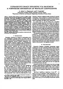
Figure 1: From left to right: one long-exposure image (time = 0.4 sec, ISO=100), one of 16 short-exposure images (time = 1/40 sec, ISO = 1600) and the average after registration. All images have been color-balanced to show the same contrast. The long exposure image is blurry due to camera motion. The middle short-exposure image is noisy, and the third one is some four times less noisy, being the result of averaging 16 short-exposure images. Images may need to be zoomed in on a screen to compare details and textures. noise variance a + bu depending on the original signal value u. Yet, this is only true for the raw CCD image. Further processing stages in the camera hardware and software such as the white balance, the demosaicking, the gamma correction, the blur and color corrections, and eventually the compression, correlate the noise and modify its nature and its standard deviation in a non trivial manner. There is therefore no noise model for JPEG images. However, as we shall see, a signal dependent noise variance model can still be estimated from bursts of JPEG images (section 4.2.) It is enough to perform reliably the average after registration (AAR).
2.1
Additive Gaussian noise estimation
Most computer vision algorithms should adjust their parameters according to the image noise level. Surprisingly, there are few papers dealing with the noise estimation problem, and most of them only estimate the variance of a signal independent additive white Gaussian noise (AWGN). This noise statistics is typically measured on the highest-frequency portion of the image spectrum, or on homogenous image patches. In the AWGN case a spectral decomposition through an orthonormal transform such as wavelets or the DCT preserves the noise statistics. To estimate the noise variance, Donoho et. al [29] consider the finest scale wavelet coefficients, followed by a median filter to eliminate the outliers. Suppose {yi }i=1,···N be N independent Gaussian random variables of zero-mean and variance σ 2 , then E{MED(|yi |)} ≈ 0.6745σ. It follows immediately that the noise standard deviation σ is given by σ ˜=
1 MED(|yi |) = 1.4826MED(|yi |). 0.6745
The standard procedure of the local approaches is to analyze a set of local estimates of the variance. For example, Rank et. al [48] take the maximum of the distribution of image derivatives. This method is based on the assumption that the underlying image has a large portion of homogeneous regions. Yet, if an image is highly textured, the noise 4
hal-00510866, version 1 - 22 Aug 2010
variance can overestimated. To overcome this problem, Ponomarenko et. al [72] have proposed to analyze the local DCT coefficients. A segmentation-based noise estimation is carried out in [1], which considers both i.i.d. and spatially correlated noise. The algorithm in [73] is a modification of the early work [72] dealing with AVIRIS (Airborne Visible Infrared Imaging Spectrometer) images, in which the evaluation of the noise variance in sub-band images is addressed. The idea is to divide each block into low frequency and high frequency components by thresholding, and to use K blocks of the smallest variance of the low frequency coefficients to calculate a noise variance, where K is adaptively selected so that it is smaller for highly-textured images. [25] proposed an improvement of the estimate of the variance of AWGN by using transforms creating a sparse representation (via BM3D [22]) and using robust statistics estimators (MAD and ICI). For a univariate data set X1 , X2 , ..., Xn , the MAD is defined as the median of the absolute deviations from the data’s median: MAD = mediani ( |Xi − medianj (Xj )| ) . The algorithm is as follows. 1. for each 8 × 8 block, group together up to 16 similar non-overlapping blocks into 3D array. The similarity between blocks in evaluated by comparing corresponding blocks extracted from a denoised version by BM3D. 2. apply a 3-D orthonormal transform (DCT or wavelet) on each group and sort the coefficients according to the zig-zag scan. 3. collect the first 6 coefficients c1 , · · · , c6 and define their empirical energy as the mean of the magnitude of the (up to 32) subsequent coefficients: E{|cj |2 } = mean{|c2j+1 , · · · , c2j+32 |} 4. Sort the coefficients from all the groups (6 coefficients per group) according to their energy 5. do MAD and Intersection of Confidence Intervals (ICI) [42] to achieve the optimal bias-variance trade-off in the MAD estimation. All the above mentioned algorithms give reasonable estimates of the standard deviation when the noise is uniform. Yet, when applying these algorithms to estimate signal dependent noise, the results are poor. The work of C. Liu et. al. [54] estimates the upper bound on the noise level fitting to a camera model. The noise estimation from the raw data is discussed in [39, 40]. The former is a parametric estimation by fitting the model to the additive Poissonian-Gaussian noise from a single image, while the latter measures the temporal noise based on an automatic segmentation of 50 images.
2.2
Poisson Noise Removal
This paper deals with real noise, which in most real images (digital cameras, tomography, microscopy and astronomy) is a Poisson noise. The Poisson noise is inherent to photon counting. This noise adds up to a thermal noise and an electronic noise which are approximately AWGN. In the literature algorithms considering the removal of AWGN are dominant but, if its model is known, Poisson noise can be approximately reduced to AWGN by a so called variance stabilizing transformation (VST). The standard procedure follows three steps, 1. apply VST to make the data homoscedastic 5
2. denoise the transformed data 3. apply the inverse VST.
hal-00510866, version 1 - 22 Aug 2010
The square-root operation is widely used as a VST, √ f (z) = b z + c.
(1)
It follows from the asymptotic unit variance of f (z) that the parameters are given by b = 2 and c = 3/8, which is the Anscombe transform [2]. A multiscale VST (MS-VST) is studied in [91] along with the conventional denoising schemes based on wavelets, ridgelets and curvelets depending on morphological features (isotropic, line-like, curvilinear, etc) of the given data. It is argued in [58] that the inverse transformation of VST is crucial to the denoising performance. Both the algebraic inverse � �2 3 D − . IA (D) = 2 8 and the asymptotically unbiased inverse IB (D) =
�
D 2
�2
1 − , 8
in [2] are biased for low counts. The authors [58] They consider an inverse transform IC that maps value Ez|y that r ∞ X 3 E{f (z)|y} = 2 z+ 8 z=0
propose an exact unbiased inverse. the value E{f (z)|y} to the desired y z exp−y · z!
!
where f (z) is the forward Anscombe transform (1). In practice, it is sufficient to compute the above equation for a limited set of values y and approximate IC by IB for large values of y. Furthermore, the state-of-the-art denoising scheme BM3D [39] is applied in the second step. There are also wavelets based methods [69, 50] or Bayesian [80, 56, 51] removing Poisson noise. In particular, the wavelet-domain Wiener filter [69] uses a cross-validation that not only preserves important image features, but also adapts to the local noise level of the spatially varying Poisson process. The shrinkage of wavelet coefficients investigates how to correct the thresholds [50] to explicitly account for effects of the Poisson distribution on the tails of the coefficient distributions. A recent Bayesian approach by Lefkimmiatis et al. [51] explores a recursive quad-tree image representation which is suitable for Poisson noise degradation and then follows an expectation-maximization technique for parameter estimation and Hidden Markov tree (HMT) structures for interscale dependencies. The common denominator to all such methods is that we need an accurate Poisson model, and this will be thoroughly discussed in Section 4. It is, however, a fact that the immense majority of accessible images are JPEG images which contain a noise altered by a long chain of processing algorithms, ending with compression. Thus the problem of estimating noise in a single JPEG image is extremely ill-posed. It has been the object of a thorough study in [53]. This paper proposes a blind estimation and removal method of color noise from a single image. The interesting feature is that it constructs a “noise level function” which is signal dependent, obtained by computing empirical standard deviations image homogeneous segments. Of course the remanent noise in a JPEG image is no way white or homogeneous, the high frequencies 6
being notoriously removed by the JPEG algorithm. On the other hand, demosaicking usually acts as a villainous converter of white noise into very structured colored noise, with very large spots. Thus, even the variance of smooth regions cannot give a complete account of the noise damage, because noise in JPEG images is converted in extended flat spots. We shall, however, retain the idea promoted in [53] that, in JPEG images, a signal dependent model for the noise variance can be found. In section 4.2 a simple algorithm will be proposed to estimate the color dependent variance in JPEG images from multi-images. All in all, the problem of estimating a noise variance is indeed much better posed if several images of the same scene by the same camera, with the same camera parameters, are available. This technique is classic in lab camera calibration [44].
hal-00510866, version 1 - 22 Aug 2010
3
Multi-images and super resolution algorithms
Photo stitching Probably one of the most popular applications in image processing, photo stitching [14, 57] is the first method to have popularized the SIFT method permitting to register into a panorama a set of image of a same scene. Another related application is video stabilization [7]. In these applications no increase in resolution is gained, the final image has roughly the same resolution as the initial ones. Super-resolution Super-resolution means creating a higher resolution, larger image from several images of the same scene. Thus, this theme is directly related to the denoising of image bursts. It is actually far more ambitious, since it involves a deconvolution. However, we shall see that most super-resolution algorithms actually make a moderate zoom in, out of many images, and therefore mainly perform a denoising by some sort of accumulation. The convolution model in the found references is anyway not accurate enough to permit a strong deconvolution. A single-frame super-resolution is often referred to as interpolation. See for example [85, 86]. But several exemplar-based super-resolution methods involve other images which are used for learning, like in Baker and Kanade [4] who use face or text images as priors. Similarly, the patch-example-based approaches stemming from the seminal paper [41], use a nearest-neighbor search to find the best match for local patches, and replace them with the corresponding high-resolution patches in the training set, thus enhancing the resolution. To make the neighbors compatible, the belief-propagation algorithm to the Markov network is applied, while another paper [26] considered a weighted average by surrounding pixels (analogue to nonlocal means [15]). Instead of a nearest-neighbor search, Yang et. al [83] proposed to incorporate the sparsity in the sense that each local patch can be sparsely represented as a linear combination of low-resolution image patches; and a high-resolution image is reconstructed by the corresponding high-resolution elements. The recent remarkable results of [87] go in the same direction. The example-based video enhancement is discussed in [12], where a simple frame-by-frame approach is combined with temporal consistency between successive frames. Also to mitigate the flicker artifacts, a stasis prior is introduced to ensure the consistency in the high frequency information between two adjacent frames. Focus on registration In terms of image registration, most of the existing superresolution methods rely either on a computationally intensive optical flow calculation, or on a parametric global motion estimation. The authors of [94] discuss the effects of multi-image alignment on super-resolution. The flow algorithm they employ addresses 7
hal-00510866, version 1 - 22 Aug 2010
two issues: flow consistency (flow computed from frame A to frame B should be consistent with that computed from B to A) and flow accuracy. The flow consistency can be generalized to many frames by computing a consistent bundle of flow fields. Local motion is usually estimated by optical flow, other local deformation models include Delaunay triangulation of features [9] and B-splines [64]. Global motion, on the other hand, can be estimated either in the frequency domain or by feature-based approaches. For example, Vandewalle et. al. [82] proposed to register a set of images based on their low-frequencies, aliasing-free part. They assume a planar motion, and as a result, the rotation angle and shifts between any two images can be precisely calculated in the frequency domain. The standard procedure for feature-based approaches is (1) to detect the key points via Harris corner [19, 3] or SIFT [89, 75], (2) match the corresponding points while eliminating outliers by RANSAC and (3) fit a proper transformation such as a homography. The other applications of SIFT registration are listed in Tab. 2. Reconstruction after registration A number of papers focus on image fusion, assuming the motion between two frames is either known or easily computed. Elad and Feuer [34] formulate the super-resolution of image sequences in the context of Kalman filtering. They assume that the matrices which define the state-space system are known. For example, the blurring kernel can be estimated by a knowledge of the camera characteristics, and the warping between two consecutive frames is computed by a motion estimation algorithm. But due to the curse of dimensionality of the Kalman filter, they can only deal with small images, e.g. of size 50 × 50. The work [59] by Marquina and Osher limited the forward model to be spatial-invariant blurring kernel with the down-sampling operator, while no local motion was present. They solved a TV-based reconstruction with Bregman iterations. A joint approach on demosaicing and super-resolution of color images is addressed in [35], based on their early super-resolution work [36]. The authors use the bilateral-TV regularization for the spatial luminance component, the Tikhonov regularization for the chrominance component and a penalty term for inter-color dependencies. The motion vectors are computed via a hierarchical model-based estimation [10]. The initial guess is the result of the Shift-And-Add method. In addition, the camera PSF is assumed to be a Gaussian kernel with various standard deviation for different sets of experiments. Methods joining denoising, deblurring, and motion compensation Super-resolution and motion deblurring are crossed in the work [5]. First the object is tracked through the sequence, which gives a reliable and sub-pixel segmentation of a moving object [6]. Then a high-resolution is constructed by merging the multiple images with the motion estimation. The deblurring algorithm, which mainly deals with motion blur [47], has been applied only to the region of interest. The recent paper on super-resolution by L. Baboulaz and P. L. Dragotti [3] presents several registration and fusion methods. The registration can be performed either globally by continuous moments from samples, or locally by step edge extraction. The set of registered images is merged into a single image to which either a Wiener or an iterative Modified Residual Norm Steepest Descent (MRNSD) method is applied [67] to remove the blur and the noise. The super-resolution in [75] uses SIFT + RANSAC to compute the homography between the template image and the others in the video sequence, shifts the low-resolution image with subpixel accuracy and selects the closest image with the optimal shifts.
8
hal-00510866, version 1 - 22 Aug 2010
Implicit motion estimation More recently, inspired by the nonlocal movie denoising method, which claims that “denoising images sequences does not require motion estimation” [16], researchers have turned their attention towards super-resolution without motion estimation [32, 31, 74]. Similar methodologies include the steering kernel regression [78], BM3D [24] and its many variants. The forward model in [24] does not assume the presence of the noise. Thus the authors pre-filter the noisy LR input by V-BM3D [21]. They up-sample each image progressively m times, and at each time, the initial estimate is obtained by zero-padding the spectra of the output from the previous stage, followed by filtering. The overall enlargement is three times the original size. Super-resolution in both space and time is discussed in [76, 77], which combine multiple low-resolution video sequences of the same dynamic scene. They register any two sequences by a spatial homography and a temporal affine transformation, followed by a regularization-based reconstruction algorithm. A synoptic table of super-resolution multi-images methods Because the literature is so rich, a table of the mentioned methods, classified by their main features, is worth looking at. The methods can be characterized by a) their number k of fused images, which goes from 1 to 60, b) the √ zoom factor, usually 2 or 3, and therefore far inferior to the potential zoom factor k, c) the registration method, d) the deblurring method, e) the blur kernel. A survey of the table demonstrates that a majority of the methods use many images to get a moderate zoom, meaning that the denoising factor is important. Thus, these methods denoise in some sense by accumulation. But, precisely because all of them aim at super-resolution, none of them considers the accumulation by itself. Tables 1 and 2 confirm the dominance of SIFT+RANSAC as a standard way to register multi-images, as will also be proposed here in an improved variant. Several of the methods in Table 1 which do not perform SIFT+RANSAC, actually the last four rows, are “implicit”. This means that they adhere to the dogma that denoising does not require motion estimation. It is replaced by multiple block motion estimation, like the one performed in NL-means and BM3D. However, we shall see in the experimental section that AAR (average after registration) has a still better performance than such implicit methods. This is one of the main questions that arose in this exploration, and the answer is clear cut: denoising by accumulation, like in ancient photography times still is a valid response in the digital era.
4
Noise blind estimation
In this section we return to noise estimation and will confront and cross-validate a single frame noise estimation with a multi-images noise estimation.
4.1
Single image noise estimation
Most noise estimation methods have in common that the noise standard deviation is computed by measuring the derivative or equivalently the wavelet coefficient values of the image. As we mentioned, Donoho et al. [30] proposed to estimate the noise standard deviation as the median of absolute values of wavelet coefficients at the finest scale. Instead of the median, many authors [13, 49] prefer to use a robust median. Olsen [70] and posteriorly Rank et al. [48] proposed to compute the noise standard deviation by taking a robust estimate on the histogram of sample variances of patches 9
Table 1: comparison of Super Resolution algorithms Ref.
hal-00510866, version 1 - 22 Aug 2010
[41] [4] [26] [83] [19] [18] [94] [82] [34] [36, 35] [75]* [89] [5] [3] [32] [31] [74] [78] [24]
# of images V.S. factor 1 2 to 16 1 2 3 1 to 4 15 2 25 3 40 2 4 2 100 2 30 3 15, 60 2 20 4 10 2 20, 40 8 1 20 30
2 3 3
9
3
Registration
Deblurring
KNN to training set
blur kernel NO
MAP penalty
3×3 5×5 Not mention Not mention
sparse w.r.t. traning Harris+RANSAC PCA consistent flow bundle frequency domain assume known motion hierarchical estimates [10] SIFT+RANSAC SIFT+RANSAC region tracking [6] moment-based or Harris + RANSAC implicit: NLM
back-projection Tiknonov
implicit: NLM kernel regression Video-BM3D
TV bilateral-TV zero-padding spectra
NO NO NO Kalman filter bilateral-TV
3 × 3 average Gaussian
NO Least-square motion analysis [47] Wiener or MRNSD [67] NO
Gauss(σ = 3) motion blur B-spline of degree 7
3 × 3 average 3 × 3 average
Table 2: Multi-image SIFT for registration [8]* [64] [84] [46] [52] [93]
Application manuscript registration Mosaic stitching head tracking
# of images Not mention 30 ultrasound 60 MRI 200 10 6 1020
Registration SIFT + RANSAC SIFT + threshold + least-square for affine SIFT + RANSAC
Blending method Delaunay triangulation B-splines deformation
SIFT + RANSAC SIFT + RANSAC
weighted average NA (track 3D motion)
10
weighted average
hal-00510866, version 1 - 22 Aug 2010
in the derivative image. In order to minimize the effect of edges small windows were preferred, with 3 × 3 or 5 × 5 pixels. The sample variance of small patches or the pointwise derivatives provide a non robust measure and require a considerable number of samples with few outliers to guarantee the correct selection of the standard deviation. We observed that the opposite point of view, that is, the use of larger windows 15 × 15 pixels to 21 × 21 pixels permits a more robust estimation. However, since larger windows may contain more edges a much smaller percentile will be preferred to the median, in practice the 1% or the 0.5%. Noise in real photograph images is signal dependent. In order to adapt the noise estimation strategies, the gray level image histogram will be divided adaptively into a fixed number of bins having all the same number of samples. This is preferable to classical approaches where the gray range is divided into equal intervals. Such a uniform division can cause many bins to be almost empty. To evaluate if a signal dependent noise can be estimated from a single image, 110 images were taken with a Nikon D80, with ISO 100 and very good illumination conditions. These are the best conditions we can expect to have a low noise standard deviation. These color images were converted to gray level by averaging the three color values at each pixel. Finally factor 3 sub-sampling was applied by averaging square groups of nine pixels. These operations having divided the noise standard deviation by slightly more than five, these images can be considered as noise free. Finally, a signal dependent noise was added to them, with variance 8 + 2u where u was the noiseless grey level. The uniform and adaptive divisions of the grey level range in a fixed number of 15 bins were compared, and several noise estimation methods were applied to estimate the noise standard deviation inside each bin. The performance of all methods are compared in Table 3 showing the average and standard deviation of the errors between the estimated and original noise curves. The best estimate is obtained by applying the proposed strategy using the variance of large patches rather than small ones or point derivatives. These measurements also confirm that the division of the grey level range into bins with fixed cardinality is preferable to the fixed length interval division. This experiment confirms that a signal dependent noise can be estimated with a high accuracy. Ground truth? In order to evaluate the performance of such a noise estimation algorithm in real images we need a ground truth to compare with. This ground truth can be obtained for a given camera by taking a sequence of images of the same pattern, after fixing the camera on a pedestal. All camera parameters remain unchanged for all photographs of the sequence, thus avoiding different exposure times or apertures. The temporal average and standard deviation of the whole sequence of images can therefore be computed without any further registration. The use of a piecewise constant image reduces the effect of small vibrations of the camera, see Fig. 2. The noise in each channel is estimated independently. Each color range is divided adaptively into a fixed number of bins taking into account the color channel histogram. Inside each bin a percentile is used to estimate the standard deviation. Fig. 3 displays the ground truth estimated curves with this strategy, both in RAW and JPEG format for two different ISO settings. The ground truth curves are compared with the ones estimated in the first image of the sequence by the proposed single image noise estimation algorithm. For the RAW case, the single image and ground truth estimated curves are nearly identical. Fig. 2 shows a lack of red in the RAW image of the calibration pattern, even if this pattern is actually gray. This effect is corrected by the white balance as observed in the JPEG image.
11
hal-00510866, version 1 - 22 Aug 2010
e std(e)
MAD RMAD MVPD MVPD2 1.81 2.87 1.58 0.75 1.14 2.59 1.06 0.61 a) Uniform gray division
e std(e)
MAD RMAD MVPD MVPD2 1.66 1.87 1.36 0.73 1.04 1.17 0.90 0.35 b) Adaptive gray division
Table 3: A signal dependent noise with variance 8 + 2u is added to 110 noise free images. The uniform and adaptive strategies for dividing the grey level range in a fixed number of 15 bins are compared. For each strategy, the following noise estimation methods in each bin are compared: median of absolute derivatives (MAD), robust median of absolute derivatives (RMAD), median of sample variance of patches 3×3 of the derivative image (MVPD) and 0.005 percentile of sample variance of patches 21×21 of the derivative image (MVPD2). Are displayed the average and standard deviation of the errors between the estimated and original noise curves for the 110 images. The ground truth noise curves estimated from the JPEG images do not agree at all with the classical noise model. This is due to the various image range nonlinear transformations applied by the camera hardware during the image formation, which modify the nature and standard deviation of the noise. The ground truth and single image estimated curves in the JPEG case have a similar shape but a different magnitude. The main new feature is that the interpolation and low pass filtering applied to the originally measured values have strongly altered the high frequency components of the noise. Thus, the noise statistics are no longer computable from a local patch of the image. The estimation of such a noise curve can only be accomplished by computing the temporal variance in a sequence of images of the same scene.
Figure 2: Calibration pattern used for noise ground truth estimation. Left: raw image. Right: JPEG image. Even if the calibration pattern is nearly gray the raw image looks blue because the red is less present. This effect is corrected by the white balance applied by the camera image chain leading to the jpeg image.
4.2
Multi-image noise estimation
A temporal average requires the images of the sequence to be perfectly registered. Yet, this registration rises a serious technical objection: how to register globally the images of a burst? Fortunately, there are several situations where the series of snapshots are 12
35
35
5
ISO 400
30
25
25
20
20
15
15
10
5
ISO 400
ISO 400
4.5
4.5
4
4
3.5
3.5
3
3
2.5
2.5
2
2
1.5
1.5
1
1
0.5
0.5
10
0
200
400
600
800
1000
1200
60
5
0
200
400
600
800
1000
0 20
1200
60
60
80
100
120
140
160
55
50
50
45
45
40
40
35
35
0 20
180
40
60
80
100
120
140
160
180
200
5
ISO 800
55
30
40
5
ISO 800
ISO 800
ISO 800
4.5
4.5
4
4
3.5
3.5
3
3
2.5
2.5
2
2
1.5
1.5
30
25
25
20
20
15
15
0
500
1000
1500
2000
2500
0
500
1000
1500
2000
1
1
0.5
0.5
0 40
2500
a) RAW images
hal-00510866, version 1 - 22 Aug 2010
5
ISO 400
30
60
80
100
120
140
160
180
200
220
240
0 40
60
80
100
120
140
160
180
200
220
240
b) JPEG images
Figure 3: Ground truth and single image noise estimates for the RAW and JPEG images of Fig. 2. The estimated curve by the temporal average and standard deviation coincide with the one estimated from the first image by the proposed single image noise estimation algorithm. This is not the case for the JPEG images. The ground truth and single image estimated curves in the JPEG case have a similar shape but a different magnitude. The interpolation and low pass filtering applied to the original measured values have altered the high frequency components of the noise and have correlated its low frequencies. This means that the noise statistics are no longer computable from a local patch of the image. The estimation of a noise curve can only be accomplished by computing the temporal variance in a sequence of images of the same scene. indeed related to each other by a homography, and we shall explore these situations first. The homography assumption is actually valid in any of the following situations: 1. the only motion of the camera is an arbitrary rotation around its optic center; 2. the photographed objects share the same plane in the 3D scene; 3. the whole scene is far away from the camera. The computation of an homography between a pair of images needs the accurate correspondence of at least four points in each image. Finding key points in images and matching them is a fundamental step for many computer vision and image processing applications. One of the most robust is the Scale Invariant Feature Transform (SIFT) [55], which we will use. Other possible methods allowing for large baselines are [61, 62, 60, 71, 66, 65], but we are here using images taken with only slight changes of view point. Because wrong matches occur in the SIFT method, an accurate estimate of the dominant homography will require the elimination of outliers. The standard method to eliminate outliers is RANSAC (RANdom SAmple Consensus) [38]. However, it is efficient only when outliers are a small portion of the whole matching set. For this reason several variants have been proposed to improve the performance of outlier elimination, the principal being [79, 90, 81, 68, 63]. The main difference between our approach and the classic outlier elimination is the fact that we dispose of a whole sequence of images and not just of a pair. Instead of choosing a more elaborate version than RANSAC, we preferred to exploit the sequence redundancy in order to improve the registration stage. 13
The goal is to estimate a dominant homography for the whole set of images, which are typically a few dozens. Only matches which are common to the whole sequence must be kept. In other terms, the keypoints of the first image are kept only if they are matched with another keypoint in any other image of the sequence. This constraint eliminates most of the outliers (see Algorithm 1). In order to apply such a strategy, we assume that the images overlap considerably. Recall that the purpose is not to make a mosaic or a panorama, but to estimate the noise curve and eventually to denoise the sequence. A temporal average and standard deviation is computed for the registered sequence. The average values are used to build a histogram and to divide the grey level range adaptively. Inside each bin, the median value of the corresponding standard deviations is taken.
hal-00510866, version 1 - 22 Aug 2010
Algorithm 1 Hybrid Accumulation After Registration Algorithm Input Initial set of images I0 , I1 , · · · , In , obtained from a burst SIFT Apply the SIFT algorithm between to each pair (I0 , Ij ), j = 1, · · · , n. Call Sj the set of matches. Retain from Sj only the matches for which the matching key point in I0 has a match in all other images. RANSAC Set number of agreed points, m, to 0. while the number of trials does not exceed N do Pick up 4 random points from S0 for (each j > 0) do Compute the homography using these 4 points and the corresponding ones in Sj Add to m the number of points in Sj which agree with this homography up to the precision p. end for If m > maxim, then maxim = m and save the set of agreed points in the whole sequence end while Compute for each pair, the homography Hj with the selected points. FUSION Apply the homography Hj to each image obtaining I¯j , j = 1, · · · , n. Average the transformed images obtaining the mean µ(x, y). Compute also σ(x, y), the temporal standard deviation. Estimate the noise curve using σ(x, y), getting σn (u) the standard deviation associated to each color u. Obtain the final estimate: (1 − w(µ, σ))µ(x, y) + w(µ, σ) NL(I0 )(x, y), where NL is the NL-means algorithm (Buades et al. [15]) and the function w(ν, σ) is defined by 0 if σ < 1.5σn (µ) σ−1.5σn (µ) if 1.5σ w(ν, σ) = n (µ) < σ < 3σn (µ) 1.5σn (µ) 1 if σ > 3σn (µ) 14
hal-00510866, version 1 - 22 Aug 2010
Fig. 4 displays three frames from an image sequence with a rotating pattern and a fixed pedestal. The noise curves estimated from the first image with the single image algorithm and those from the registered and averaged sequence are displayed in the same figure. The estimated curves in the raw image coincide if either of both strategies is applied. However, as previously observed these are quite different when we take into account the JPEG image.
90
90
80
80
70
70
60
60
50
50
40
40
30
30
20
20
10 0
10
0
500
1000
1500
2000
2500
3000
0
3500
10
10
9
9
8
8
7
7
6
6
5
5
4
4
3
3
2
2
1 0
0
500
1000
1500
2000
2500
3000
3500
1
0
50
100
150
200
0
250
0
50
100
150
200
250
Figure 4: Three frames from an image sequence with a rotating pattern and a fixed pedestal both in RAW (top) and JPG (bottom). The estimated curves in the raw image coincide if either of both strategies is applied. However, as previously observed these are quite different when we take into account the JPEG image Images taken with indoor lights often show fast variations of the contrast and brightness, like those in Fig. 5. This brightness must be rendered consistent through all the images, so that the standard deviation along time is due to the noise essentially and not to the changes of lights. For this reason, a joint histogram equalization must conservatively be applied before the noise estimation chain. The Midway equalization method proposed in [27, 28] is the ideal tool to do so, since it forces all images to adopt a joint 15
15
10
5
0
0
10
20
30
40
50
60
70
80
90
100
0
10
20
30
40
50
60
70
80
90
100
15
10
5
hal-00510866, version 1 - 22 Aug 2010
0
Figure 5: Top: two frames of an image sequence with variations of brightness. Noise curve estimated by temporal average and standard deviation after registration. Bottom: the same two frames of the sequence after a joint histogram equalization [28] and estimated noise curves. The second estimation is correct. The first was not, because of the almost imperceptible lighting conditions. midway histogram which is indeed a kind of barycenter of the histograms of all images in the burst. Fig. 5 illustrates the noise estimation after and before color equalization.
5
Average after registration denoising
The core idea of the average after registration (AAR) denoising method is that the various values at a cross-registered pixels obtained by a burst are i.i.d.. Thus, averaging the registered images amounts to averaging several realizations of these random variables. √ An easy calculation shows that this increases the SNR by a factor proportional to n, where n is the number of shots in the burst. There is a strong argument in favor of denoising by simple averaging of the registered samples instead of block-matching strategies. If a fine non-periodic texture is present in an image, it is virtually indistinguishable from noise, and actually contains a flat spectrum part which has the same Fourier spectrum as the white noise. Such fine textures can be distinguished from noise only if several samples of the same texture are present in other frames and can be accurately registered. Now, state of the art denoising methods (e.g. BM3D) are based on nonlocal block matching, which is at risk to confound the repeated noise-like textures with real noise. A registration process which is far more global than block matching, using strong features elsewhere in the image, should permit a safer denoising by accumulation, provided the registration is sub-pixel accurate and the number of images sufficient. A simple test illustrates this superior noise reduction and texture preservation on fine non periodic textures. A image was randomly translated by non integer shifts, and signal dependent noise was added to yield an image sequence of sixteen noisy images. Figure 6 shows the first image of the sequence and its denoised version obtained by accumulation after registration (AAR). The theoretical noise reduction factor with sixteen images is 16
hal-00510866, version 1 - 22 Aug 2010
four. This factor is indeed reached by the accumulation process. Table 4 displays the mean square error between the original image and the denoised one by the different methods. Block based algorithms such as NLmeans [15] and BM3D [23], have a considerably larger error, even if their noise reduction could be theoretically superior due to their two dimensional averaging support. But fine details are lost in the local comparison of small image blocks.
Figure 6: Noise curve. From top to bottom: one of the simulated images by moving the image and adding Poisson noise, denoised by accumulation after registration and the noise curve obtained by the accumulation process using the sixteen images. The standard deviation of the noise (Y-axis) fits to the square root of the intensity (X-axis). As mentioned in the introduction, the registration by using the SIFT algorithm and computing a homography registration is by now a standard approach in the image fusion literature. The main difference of the proposed approach with anterior work is that the mentioned works do not account for registration errors. Yet, in general, the images of a 3D scene are not related by a homography, but by an epipolar geometry [43]. Even if the camera is well-calibrated, a 3D point-to-point correspondence is impossible to obtain without computing the depth of the 3D scene. However, as we mentioned, a camera held steadily in the hand theoretically produces images deduced from each other by a homography, the principal image motion being due to slight rotations of the camera. Nonetheless, we should not expect that a simple homography will be perfectly accurate everywhere in each pair, but only on a significant part. A coherent registration will be obtained by retaining only the SIFT matches that are common to the whole burst. Therefore the registration applies a joint RANSAC strategy, as exposed in Algorithm 1. This ensures that the same background objects are used in all images to compute the corresponding homographies. 17
noisy NLM BM3D AR
Barbara 11.30 4.52 4.33 3.55
Couple 11.22 3.73 3.39 3.03
Hill 10.27 4.50 3.90 2.73
hal-00510866, version 1 - 22 Aug 2010
Table 4: Mean square error between the original image and the denoised one by the various considered methods applied on the noisy image sequences in Figure 6. The block based algorithms, NLmeans [15] and BM3D [23] have a considerably larger error, even if their noise reduction could be in theory superior, due to their two dimensional averaging support. AAR is close to the theoretical reduction factor four. The main new feature of the algorithm is this: The averaging is applied only at pixels where the observed standard deviation after registration is close to the one predicted by the estimated noise model. Thus, there is no risk whatsoever associated with AAR, because it only averages sets of samples whose variability is noise compatible. At the other pixels, the conservative strategy is to apply a state of the art video denoising algorithm such as the spatiotemporal NL-means algorithm or BM3D. To obtain a smooth transition between the averaged pixels and the NL-means denoised pixels, a weighting function is used. This function is equal to 0 when the standard deviation of the current pixel is lower than 1.5 times the estimated noise standard deviation, and equal to 1 if it is larger than 3 times the estimated noise standard deviation. The weights are linearly interpolated between 1.5 and 3.
6
Discussion and experimentation
We will compare the visual quality of restored images from real burst sequences. The focus is on JPEG images, which usually contain non white noise and color artifacts. As we illustrated in the previous sections, the variability of the color at a certain pixel cannot be estimated from a single image but from a whole sequence. We will compare the denoised images by using AAR as well as the classical block based denoising algorithms, NL-means. Fig. 7 shows the results obtained on three different bursts. Each experiment shows in turn: a) three images extracted from the burst, b) the burst average after registration performed at all points, followed by a mask of the image regions in which the temporal standard deviation is significantly larger than the standard deviation predicted by the noise estimate. At all of these points a block based denoising estimate is used instead of the temporal mean. The final combined image, obtained by an hybridization of the average registration and NL-Means or BM3D, is the right image in each second row. The first experimental data was provided by the company DxO Labs. It captures a rotating pattern with a fixed pedestal. In this case, the dominant homography is a rotation of the main circular pattern, which contains more SIFT points than the pedestal region. Since the proposed algorithm only finds a dominant homography, which is the rotation of the pattern, the simple average fails to denoise the region of the fixed pedestals and of the uniform background. As shown in the white parts of the mask, these regions are detected because they have an excessive temporal standard deviation. They are therefore treated by NL-means or BM3D in the final hybrid result. The whole pattern itself is restored by pure average after registration. The second burst consists of two books, a newspaper and a moving mouse. Since the 18
dominant homography is computed on still parts, the books and the background, the moving mouse is totally blurred by the averaging after registration, while the rest of the scene is correctly fused. As a consequence, AAR uses the average everywhere, except the part swept by the mouse. The last burst is a sequence of photographs with short exposure time of a large painting taken in Mus´ee d’Orsay, Martyrs chr´etiens entrant lamphith´eˆ atre by L´eon B´enouville. Making good photographs of paintings in the dim light of most museums is a good direct application for the proposed algorithm, since the images of the painting are related by a homography even with large changes of view point, the painting being flat. As a result, the average is everywhere favored by the hybrid scheme. Details on the restored images and comparison with BM3D are shown in Fig. 8-10. Dim light images are displayed after their color values have been stretched to [0, 255].
hal-00510866, version 1 - 22 Aug 2010
References [1] Sergey K. Abramov, Vladimir V. Lukin, Benoit Vozel, Kacem Chehdi, and Jaakko T. Astola. Segmentation-based method for blind evaluation of noise variance in images. J. Appl. Remote Sens., 2(1), 2008. [2] F. J. Anscomb. The transformation of poisson, binomial and negative-binomial data. Biometrika, 35(3):246–254, 1948. [3] L. Baboulaz and P. L. Dragotti. Exact feature extraction using finite rate of innovation principles with an application to image super-resolution. IEEE Transactions on Image Processing, 18(2):281–298, 2009. [4] Simon Baker and Takeo Kanade. Limits on super-resolution and how to break them. IEEE Trans. Pattern Anal. Mach. Intell., 24(9):1167–1183, 2002. [5] B. Bascle, Andrew Blake, and Andrew Zisserman. Motion deblurring and superresolution from an image sequence. In ECCV ’96: Proceedings of the 4th European Conference on Computer Vision-Volume II, pages 573–582, 1996. [6] Benedicte Bascle, Benedicte Bascle, Rachid Deriche, Rachid Deriche, and Projet Robotvis. Region tracking through image sequences. In In Proc. 5th Int. Conf. on Computer Vision, pages 302–307, 1995. [7] S. Battiato, G. Gallo, G. Puglisi, and S. Scellato. SIFT features tracking for video stabilization. In Image Analysis and Processing, 2007. ICIAP 2007. 14th International Conference on, pages 825–830, 2007. [8] R. Baumann and W. B. Seales. Robust registration of manuscript images. In JCDL ’09: Proceedings of the 9th ACM/IEEE-CS joint conference on Digital libraries, pages 263–266, New York, NY, USA, 2009. ACM. [9] Ryan Baumann and W. Brent Seales. Robust registration of manuscript images. In JCDL ’09: Proceedings of the 9th ACM/IEEE-CS joint conference on Digital libraries, pages 263–266, New York, NY, USA, 2009. ACM. [10] James R. Bergen, P. Anandan, Keith J. Hanna, and Rajesh Hingorani. Hierarchical model-based motion estimation. In ECCV ’92: Proceedings of the Second European Conference on Computer Vision, pages 237–252, 1992. 19
[11] M. Bertalmio and S. Levine. Fusion of bracketing pictures. In Proceedings of the 6th Conference on Visual Media Production. [12] Christopher M. Bishop, Andrew Blake, and Bhaskara Marthi. Super-resolution enhancement of video. In In Proc. Artificial Intelligence and Statistics, 2003. [13] M.J. Black and G. Sapiro. Edges as outliers: Anisotropic smoothing using local image statistics. Lecture notes in computer science, pages 259–270, 1999. [14] Matthew Brown and David G. Lowe. Automatic panoramic image stitching using invariant features. International Journal of Computer Vision, pages 59–73, 2007. [15] A. Buades, B. Coll, and J. M. Morel. A review of image denoising algorithms, with a new one. Multiscale Modeling Simulation, 4(2):490–530, 2005.
hal-00510866, version 1 - 22 Aug 2010
[16] A. Buades, B. Coll, and J.M. Morel. Nonlocal image and movie denoising. International Journal of Computer Vision, 76(2):123–139, 2008. [17] T. Buades, Y. Lou, JM Morel, and Z. Tang. A note on multi-image denoising. Int. workshop on Local and Non-Local Approximation in Image Processing, pages 1–15, August 2009. [18] D. Capel and A. Zisserman. Super-resolution from multiple views using learnt image models. In Computer Vision and Pattern Recognition, 2001. CVPR 2001. Proceedings of the 2001 IEEE Computer Society Conference on, volume 2, pages II–627–II– 634, 2001. [19] David Capel and Andrew Zisserman. Automated mosaicing with super-resolution zoom. In In Proc. CVPR, pages 885–891, 1998. [20] C. Chevalier, G. Roman, and J.N. Niepce. Guide du photographe. C. Chevalier, 1854. [21] K. Dabov, A. Foi, and K. Egiazarian. Video denoising by sparse 3d transformdomain collaborative filtering. In Proc. European Signal Process. Conf., EUSIPCO, 2007. [22] K. Dabov, A. Foi, V. Katkovnik, and K. Egiazarian. Color image denoising via sparse 3d collaborative filtering with grouping constraint in luminance-chrominance space. In Proc. IEEE Int. Conf. Image Process., ICIP, 2007. [23] K. Dabov, A. Foi, V. Katkovnik, and K. Egiazarian. Image denoising by sparse 3d transform-domain collaborative filtering. IEEE Trans. Image Process., 16(8), 2007. [24] A. Danielyan, A. Foi, V. Katkovnik, and K. Egiazarian. Image And Video SuperResolution Via Spatially Adaptive Block-Matching Filtering. In Proceedings of International Workshop on Local and Non-Local Approximation in Image Processing (LNLA), 2008. [25] Aram Danielyan and A. Foi. Noise variance estimation in nonlocal transform domain. In Proceedings of International Workshop on Local and Non-Local Approximation in Image Processing, LNLA 2009. [26] Dmitry Datsenko and Michael Elad. Example-based single document image superresolution: a global map approach with outlier rejection. In Multidim System Signal Processing, number 18, pages 103–121, 2007. 20
[27] J. Delon. Movie and video scale-time equalization application to flicker reduction. Image Processing, IEEE Transactions on, 15(1):241–248, Jan. 2006. [28] Julie Delon. Midway image equalization. Journal of Mathematical Imaging and Vision, 21(2):119–134, 2004. [29] D. Donoho and J. Johnstone. Ideal spatial adaption via wavelet shrinkage. Biometrika, 81(3):425–455, 1994. [30] David Donoho and Iain M. Johnstone. Adapting to unknown smoothness via wavelet shrinkage. Journal of the American Statistical Association, 90:1200–1224, 1995.
hal-00510866, version 1 - 22 Aug 2010
[31] M. Ebrahimi and E.R. Vrscay. Multi-frame super-resolution with no explicit motion estimation. In Proceedings of the 2008 International Conference on Image Processing, Computer Vision, and Pattern Recognition, IPCV, 2008. [32] Mehran Ebrahimi and Edward Vrscay. Solving the inverse problem of image zooming using self-examples. Image Analysis and Recognition, pages 117–130, 2007. [33] E. Eisemann and F. Durand. Flash photography enhancement via intrinsic relighting. ACM Transactions on Graphics, 23(3):673–678, 2004. [34] Michael Elad and Arie Feuer. Super-resolution reconstruction of continuous image sequences. IEEE Transactions on Pattern Analysis and Machine Intelligence, 21:459–463, 1999. [35] S. Farsiu, M. Elad, and P. Milanfar. Multiframe demosaicing and super-resolution of color images. Image Processing, IEEE Transactions on, 15(1):141–159, Jan. 2006. [36] Sina Farsiu, Dirk Robinson, Michael Elad, and Peyman Milanfar. Fast and robust multi-frame super-resolution. IEEE Transactions on Image ProcessinG, 13:1327– 1344, 2003. [37] Raanan Fattal, Maneesh Agrawala, and Szymon Rusinkiewicz. Multiscale shape and detail enhancement from multi-light image collections. In ACM SIGGRAPH, page 51, 2007. [38] M. A. Fischler and R. C. Bolles. Random sample consensus: A paradigm for model fitting with applications to image analysis and automated cartography. CACM, 24(3):381–395, 1981. [39] A. Foi, S. Alenius, V. Katkovnik, and K. Egiazarian. Noise measurement for rawdata of digital imaging sensors by automatic segmentation of non-uniform targets. IEEE Sensors Journal, 7(10):1456–1461, 2007. [40] A. Foi, M. Trimeche, V. Katkovnik, and K. Egiazarian. Practical poissonian-gaussian noise modeling and fitting for single image raw-data. IEEE Transaction on Image Processing, 17(10):1737–1754, 2008. [41] William T. Freeman, Thouis R. Jones, and Egon C Pasztor. Example-based superresolution. IEEE Computer Graphics and Applications, 22:56–65, 2002. [42] A. Goldenshluger and A. Nemirovski. On spatial adaptive estimation of nonparametric regression. math. Mesh. Statistics, 6:1737–1754, 1997.
21
[43] R. I. Hartley and A. Zisserman. Multiple View Geometry in Computer Vision. Cambridge University Press, ISBN: 0521540518, second edition, 2004. [44] G. Healey and R. Kondepudy. Radiometric CCD camera calibration and noise estimation. IEEE Transactions on Pattern Analysis and Machine Intelligence, pages 267–276, 1994. [45] G.E. Healey and R. Kondepudy. Radiometric CCD camera calibration and noise estimation. IEEE Transactions on Pattern Analysis and Machine Intelligence, 16(3):267–276, 1994.
hal-00510866, version 1 - 22 Aug 2010
[46] Marko Heikkil¨ a and Matti Pietik¨ ainen. An image mosaicing module for wide-area surveillance. In VSSN ’05: Proceedings of the third ACM international workshop on Video surveillance & sensor networks, pages 11–18, New York, NY, USA, 2005. ACM. [47] Michal Irani and Shmuel Peleg. Motion analysis for image enhancement: Resolution, occlusion, and transparency. Journal of Visual Communication and Image Representation, 4:324–335, 1993. [48] M. Lendl K. Rank and R. Unbehauen. Estimation of image noise variance. In Vision, Image and Signal Processing, volume 146, pages 80–84, 1999. [49] C. Kervrann and J. Boulanger. Local Adaptivity to Variable Smoothness for Exemplar-Based Image Regularization and Representation. International Journal of Computer Vision, 79(1):45–69, 2008. [50] E. D. Kolaczyk. Wavelet shrinkage estimation of certain poisson intensity signals using corrected thresholds. Statist. Sin., 9:119–135, 1999. [51] Stamatios Lefkimmiatis, Petros Maragos, and George Papandreou. Bayesian inference on multiscale models for poisson intensity estimation: Application to photolimited image denoising. IEEE Transactions on Image Processing, 18(8):1724–1741, 2009. [52] Yanfang Li, Yaming Wang, Wenqing Huang, and Zuoli Zhang. Automatic image stitching using sift. In International Conference on Audio, Language and Image Processing (ICALIP), pages 568–571, July 2008. [53] C. Liu, R. Szeliski, S.B. Kang, C.L. Zitnick, and W.T. Freeman. Automatic estimation and removal of noise from a single image. IEEE transactions on pattern analysis and machine intelligence, 30(2):299–314, 2008. [54] Ce Liu, William T. Freeman, Richard Szeliski, and Sing Bing Kang. Noise estimation from a single image. Computer Vision and Pattern Recognition, IEEE Computer Society Conference on, 1:901–908, 2006. [55] David G. Lowe. Distinctive image features from scale-invariant keypoints. International Journal of Computer Vision, 60(2):91–110, 2004. [56] H. Lu, Y. Kim, and J.M.M. Anderson. Improved poisson intensity estimation: denoising application using poisson data. Image Processing, IEEE Transactions on, 13(8):1128–1135, Aug. 2004.
22
[57] R. Szeliski M. Brown and S. Winder. Multi-image matching using multi-scale oriented patches. International Conference on Computer Vision and Pattern Recognition, pages 510–517, 2005. [58] M. Makitalo and A. Foi. On the inversion of the anscombe transformation in lowcount poisson image denoising. In Proceedings of International Workshop on Local and Non-Local Approximation in Image Processing, LNLA 2009. [59] Antonio Marquina and S. Osher. Image super-resolution by TV-regularization and Bregman iteration. Journal of Scientific Computing, 37(3):367–382, 2008. [60] Chum O. Urban M. Matas J. and Pajdla T. Robust wide baseline stereo from maximally stable extremal regions. Proc. of British Machine Vision Conference, pages 384–396, 2002.
hal-00510866, version 1 - 22 Aug 2010
[61] K. Mikolajczyk and C. Schmid. An affine invariant interest point detector. ECCV, 1:128–142, 2002. [62] K. Mikolajczyk and C. Schmid. Scale and affine invariant interest point detectors. International Journal of Computer Vision, 60(1):63–68, 2004. [63] L. Moisan and B. Stival. A probabilistic criterion to detect rigid point matches between two images and estimate the fundamental matrix. International Journal of Computer Vision, 57(3):201–218, 2004. [64] M. Moradi, P. Abolmaesumi, and P. Mousavi. Deformable registration using scale space keypoints. In Medical Imaging 2006: Image Processing, , Proc. of SPIE, volume 6144, pages 61442G1– 61442G8, 2006. [65] J.M. Morel and G. Yu. Asift: A new framework for fully affine invariant image comparison. SIAM Journal on Imaging Science, 2(2), 2009. [66] Pablo Mus´e, Fr´ed´eric Sur, Fr´ed´eric Cao, Yann Gousseau, and Jean-Michel Morel. An a contraio decision method for shape element recognition. International Journal of Computer Vision, 69(3):295–315, 2006. [67] James Nagy and Zdenek Strakos. Enforcing nonnegativity in image reconstruction algorithms. In in Proc. SPIE Mathematical Modeling Estimation, and Imaging, pages 182–190, 2000. [68] D. Nist´er. Preemptive RANSAC for live structure and motion estimation. Machine Vision and Applications, 16(5):321–329, 2005. [69] Robert D. Nowak and Richard G. Baraniuk. Wavelet-domain filtering for photon imaging systems. IEEE Transactions on Image Processing, 8(5):666–678, 1997. [70] S. I. Olsen. Estimation of noise in images: an evaluation. CVGIP: Graph. Models Image Process., 55(4):319–323, 1993. [71] F. Sur F. Cao P. Mus´e and Y. Gousseau. Unsupervised thresholds for shape matchings. Image Precessing, 2003. Proceedings. 2003 International Conference on, 2, 2003.
23
[72] N. N. Ponomarenko, V. V. Lukin, S. K. Abramov, K. O. Egiazarian, and J. T. Astola. Blind evaluation of additive noise variance in textured images by nonlinear processing of block dct coefficients. volume 5014 of SPIE Proceedings, pages 178– 189, 2003. [73] N. N. Ponomarenko, V. V. Lukin, M. S. Zriakhov, A. Kaarna, and J. T. Astola. An automatic approach to lossy compression of AVIRIS images. IEEE International Geoscience and Remote Sensing Symposium, 2007. [74] M. Protter, M. Elad, H. Takeda, and P. Milanfar. Generalizing the non-localmeans to super-resolution reconstruction. IEEE Transactions on Image Processing, 18(1):36–51, 2009.
hal-00510866, version 1 - 22 Aug 2010
[75] Yeol-Min Seong and HyunWook Park. Superresolution technique for planar objects based on an isoplane transformation. Opt. Eng., 47, 2008. [76] E. Shechtman, Yaron Caspi, and Michal Irani. Increasing space-time resolution in video. In ECCV ’02: Proceedings of the 7th European Conference on Computer Vision-Part I, pages 753–768, 2002. [77] Eli Shechtman, Yaron Caspi, and Michal Irani. Space-time super-resolution. IEEE Trans. Pattern Anal. Mach. Intell., 27(4):531–545, 2005. [78] H. Takeda, P. Milanfar, M. Protter, and M. Elad. Super-resolution without explicit subpixel motion estimation. IEEE Transactions on Image Processing, 18(9):1958– 1975, 2009. [79] Chi-Keung Tang, Gerard G. Medioni, and Mi-Suen Lee. N-dimensional tensor voting and application to epipolar geometry estimation. IEEE Transactions on Pattern Analysis and Machine Intelligence, 23(8):829–844, 2001. [80] Klaus E. Timmermann and Robert D. Nowak. Multiscale modeling and estimation of poisson processes with application to photon-limited imaging. IEEE TRANS. ON INFO. THEORY, 45(3):846–862, 1999. [81] P. Torr and A. Zisserman. MLESAC: A new robust estimator with application to estimating image geometry. Computer Vision and Image Understanding, 78:138– 156, 2000. [82] Patrick Vandewalle, Sabine S¨ usstrunk, and Martin Vetterli. A frequency domain approach to registration of aliased images with application to super-resolution. EURASIP Journal on Applied Signal Processing, 2006:1–14, March 2006. [83] Jianchao Yang, J. Wright, T. Huang, and Yi Ma. Image super-resolution as sparse representation of raw image patches. In Computer Vision and Pattern Recognition, 2008, IEEE Conference on, pages 1–8, June 2008. [84] Zhan-Long Yang and Bao-Long Guo. Image mosaic based on sift. Intelligent Information Hiding and Multimedia Signal Processing, International Conference on, 0:1422–1425, 2008. [85] G. Yu and S. Mallat. Sparse super-resolution with space matching pursuit. In Proc. of Signal Processing with Adaptive Sparse Structured Representation (SPARS), 2009.
24
[86] G. Yu and S. Mallat. Super-resolution with sparse mixing estimators. Technical report, 2009. [87] G. Yu, G. Sapiro, and S. Mallat. Solving Inverse Problems with Piecewise Linear Estimators: From Gaussian Mixture Models to Structured Sparsity. Arxiv preprint arXiv:1006.3056, 2010. [88] Lu Yuan, Jian Sun, Long Quan, and Heung-Yeung SHum. Image deblurring with blurred/noisy image pairs. In SIGGRAPH, 2007. [89] Z. Yuan, P. Yan, and S. Li. Super resolution based on scale invariant feature transform. In Audio, Language and Image Processing, 2008. ICALIP 2008. International Conference on, pages 1550–1554, 2008.
hal-00510866, version 1 - 22 Aug 2010
[90] R. Deriche O. D. Faugeras Z. Zhang and Q.T. Luong. A robust technique for matching two uncalibrated images through the recovery of the unknown epipolar geometry. Artificial Intelligence, 78(1-2):87–119, 1995. [91] B. Zhang, M. Fadili, and J. L. Starck. Wavelet, ridgelets and curvelets for poisson noise removal. IEEE Transactions on Image Processing, 17(7):1093–1108, 2008. [92] Li Zhang, Sundeep Vaddadi, Hailin Jin, and Shree Nayar. Multiple view image denoising. In In IEEE Computer Society Conference on Computer Vision and Pattern Recognition, 2009. [93] Gangqiang Zhao, Ling Chen, Jie Song, and Gencai Chen. Large head movement tracking using sift-based registration. In MULTIMEDIA ’07: Proceedings of the 15th international conference on Multimedia, pages 807–810, New York, NY, USA, 2007. ACM. [94] W. Zhao and Harpreet S. Sawhney. Is super-resolution with optical flow feasible? In ECCV ’02: Proceedings of the 7th European Conference on Computer Vision-Part I, pages 599–613, 2002.
25
hal-00510866, version 1 - 22 Aug 2010
Figure 7: In each double row: three images of a sequence in the first row. In the second row on the left the average after registration, in the middle the mask of points with a too large temporal standard deviation, and on the right the restored image by hybrid method. These experiments illustrate how the hybrid method detects and corrects the potential wrong registrations due to local errors in the global homography.
26
hal-00510866, version 1 - 22 Aug 2010
Figure 8: Detail from image in Fig. 7. From left to right: original image, NL-means (BM3D gives a similar result) and hybrid AAR. The images may need to be zoomed in on a screen to compare details and textures. Compare the fine texture details in the trees and the noise in the sky.
Figure 9: Detail from image in Fig. 7. From left to right: original image, BM3D (considered the best state of the art video denoiser) and AAR. The images are displayed after their color values have been stretched to [0, 255]. The images may need to be zoomed in on a screen to compare details and textures. Notice how large color spots due to the demosaicking and to JPEG have been corrected in the final result.
Figure 10: Detail from image in Fig. 7. From left to right: original image, BM3D (considered the best state of the art video denoiser) and AAR. Images are displayed after their color values have been stretched to [0, 255]. The images may need to be zoomed in on a screen to compare details and textures. Compare details on the face and on the wall texture.
27
hal-00510866, version 1 - 22 Aug 2010
Figure 11: Top: initial image of the burst containing six images. Bottom: details on the initial and hybrid AAR images.
28