Index TermsâWireless Sensor Networks (WSNs), Distributed. Decoding .... The graph connectivity information .... decoding algorithm, the Viterbi algorithm for convolutional codes [8 .... ations to solve the CA problem is to follow the primal-dual.
1
In-Network Channel Decoding Using Consensus on Log-Likelihood Ratio Averages† Hao Zhu, Alfonso Cano, and Georgios B. Giannakis Department of Electrical and Computer Engineering, University of Minnesota, 200 Union Street, Minneapolis, MN 55455, USA.
Abstract—This paper considers the problem of distributed decoding of a coded message from a mobile access point (AP) sent to a sensor network. The distributed decoding problem is solved using a consensus algorithm on the log-likelihood ratio averages, which ensures that all sensors attain the same decision as if all received signals were available at a centralized location. Unlike existing distributed hypothesis testing problems, whose inter-sensor communication cost grows exponentially with the codeword size, the novel consensus-based distributed decoder exploits knowledge over the problem to reduce the cost to be linear. Link failures and inter-sensor communication noise are also accounted for. Analysis and simulations confirm that the resultant distributed decoder attains bit error rate performance approaching its centralized counterpart within a few iterations. Index Terms—Wireless Sensor Networks (WSNs), Distributed Decoding, Consensus Average
I. I NTRODUCTION We consider the problem of cooperatively decoding a message from a mobile access point (AP) by a wireless sensor network (WSN). The goal is to enforce all collaborating sensors to agree on the decoded message. Network agreement is designed so as to enable spatial diversity. Thus, the detection error at the network can be made arbitrarily small by increasing the network size, along with the codeword length. The problem of network agreement is well motivated since sensors may lack of sufficient individual processing to have a reliable message estimation on the received signal. Besides, shadowing and spatial fading may be present, naturally motivating the call for spatial diversity to compensate it. We seek for optimal local decoding with global information. We gaze this problem deriving messages to be exchanged with neighboring sensors to efficiently describe the information. Messages are derived challenged by efficiency and scalability constraints. As we will show, the optimal maximum-likelihood (ML) distributed block- and bitwise- decoding problem can be reformulated, without loss of optimality, as an equivalent problem described using log-likelihood ratios (LLR). This reformulation naturally leads to a consensus-based distributed algorithm on the LLRs which ensures that each sensor attains the same message as if all received signals were available as a centralized location. † This work was supported through collaborative participation in the Communications and Networks Consortium sponsored by the U.S. Army Research Laboratory under the Collaborative Technology Alliance Program, Cooperative Agreement DAAD19-01-2-0011. The U.S. Government is authorized to reproduce and distribute reprints for Government purposes notwithstanding any copyright notation thereon.
The distributed consensus problem has attracted great interests in the recent years. The distributed consensus averaging problem was investigated in [1], [2], from the perspective of accelerating convergence and minimizing the effects of inter-sensor noise. The consensus estimation problem has been considered by [3] the deterministic signals. The introduction of bridge sensors in [3] exploited the decomposable structure of the centralized optimization problem’s augmented Lagrangian with the method of multipliers [4]. Moreover, for the latter case noise robustness is proved both theoretically and numerically. The idea of cooperation among nodes for distributed detection problems has also attracted much attention recently. Consensus-based distributed hypothesis testing (DHT) based on the belief consensus algorithm is proposed in [5], and it is shown that this algorithm works for any connected networks with loops. This belief consensus algorithm benefits from scalability, robustness to link failures, and asynchronism in the message sent. Consensus averaging tools are also used in [6] accounting for link failures and noise robustness at the expense of slower convergence rate. From a different perspective, [7] also tackles the problem of DHT using graphical models for the probabilistic model representation. In such scenario, however, convergence may not be guaranteed for any network architecture. Network synchronism is also needed. Distributed decoding differs from the conventional view at DHT in the sense that decoding also exploits knowledge over the alphabet employed to map the messages at the AP. The novel consensus-based distributed decoder will exploit this fact to reduce communication and computation costs across the network. Specifically, compared to DHT, the novel distributed decoder will update consensus vectors of length considerably smaller than the number of hypothesis. Notation: Upper (lower) bold face letters will be used for matrices (column vectors); IN the N × N identity matrix; 1N the N × 1 all-one vector; [·]i,j is the i, jth entry of a matrix; |S| is the cardinality of the set S; CN (µ, σ 2 ) will stand for a complex Gaussian distribution with mean µ and variance σ 2 . We use p[x = z|y] to denote the probability density function (pdf) of the random variable (r.v.) x, given the r.v. y, evaluated at z. II. M ODELING & P ROBLEM F ORMULATION The problem of distributed decoding by a Cooperative Sensor Network with an AP is illustrated in Fig. 1. The AP broadcasts a common binary codeword x to an ad hoc WSN
2
Before continuing, we introduce two more assumptions. These assumptions will be later revisited and thus we name AP them for later reference: (a1) The time-invariant WSN communication graph A is connected, i.e., there exists a path connecting any two sensors on the graph; (a2) The single-hop inter-sensor communication links are ideal. Similar to [1], [2], [5] and [3], network connectivity in (a1) ensures the utilization of all informative received signal throughout the whole network by the distributed decoding algorithms. The fixed topology in (a1) and the ideal interFig. 1. Communication system with broadcasting AP and received sensors. sensor links in (a2) are assumed here for simplicity of discussions and derivations. It will turn out that our distributed decoding algorithm exhibits resilience to communication noise with J sensors. The codeword x is selected from a linear and also adapts to time-varying topologies. Simulations will (N, K) codebook C, which is assumed known at both the corroborate this. For further details, we refer the reader to [9]. AP and the sensors. Each codeword x with codelength N is encoded from the source message t of K independent III. C ONSENSUS - BASED DECODING information bits, thus the cardinality of C is 2K . For the ad The optimization variable xn in the decoder (2) only takes hoc WSN without a central unit (fusion center), the sensor j the value of either 0 or 1, thus, the following equality holds: has to rely only on its local received signal yj , as well as ½ log p[yj,n |xn = 1] if xn = 1 the single-hop communications with neighboring sensors to log p[yj,n |xn ] = log p[yj,n |xn = 0] if xn = 0 decode, via “in-network” processing, the information bearing µ ¶ message x. Let Nj ⊆ {1, . . . , J} := J denote the set of p[yj,n |xn = 1] = xn log the sensor j’s neighborhood. Inter-sensor links are assumed p[yj,n |xn = 0] to be symmetric, and the WSN is modeled as an undirected (3) + log p[yj,n |xn = 0]. graph whose vertices are the sensors and its edges represent A constant can be subtracted from the cost function in (3) the available communication links. The graph connectivity to obtain (see also [10]) information is summarized in the so-called adjacency matrix J×J A ∈ R for which [A]ji = 1 if i ∈ Nj , otherwise J X N X [A]ji = 0. The symmetry of sensor links implies A = AT . ˆ M L = arg min x γj,n xn (4) x∈C The broadcast channel from the AP to the sensor j is j=1 n=1 modeled as a discrete memoryless, and is assumed to be where γj,n denotes the LLR of each variable xn at the jth independent across sensors. We use the the conditional pdf sensor, i.e., p[yj |x] to describe the AP-to-sensor channel. We consider µ ¶ p[yj,n |xn = 0] the block decoding problem, whereby sensors infer which γj,n := log . (5) p[yj,n |xn = 1] codeword x ∈ C or information block t was broadcasted given the received signals y1 , . . . , yJ . The optimal codeword Interestingly, as already pointed out in [10] the LLR γj,n decoder is the solution of the maximum a posteriori (MAP) can be interpreted by the “cost” of decoding xn as 1 at the [8, Section 4.1]: jth sensor. In this way, it is very intuitive to see that the message
Encoder
ˆM L x
= arg max p[x|y1 , . . . , yJ ]. x∈C
(1)
Assuming that messages are equiprobable a priori, the optimal MAP decoder reduces to the maximum likelihood (ML) rule ˆ M L = arg maxx∈C p[y1 , . . . , yJ |x]. By the independence of x AP-to-sensor channels, and the memoryless of each of the the AP-to-sensor channels, we can finally write (1) as ˆ M L = arg max x x∈C
J X N X
log p[yj,n |xn ]
(2)
j=1 n=1
where yj,n (xn ) denotes the nth entry of yj (x). Our goal is to develop a distributed decoding algorithm with affordable inter-sensor communications and low computational costs, in order to acquire the centralized optimal decoder in (2) in every sensor.
centralized ML decoding problem (4) is to find a codeword ˆ M L with the minimum “decoding cost”, i.e., the maximum x overall likelihood ratio. Defining the LLR vector at the jth sensor γ j := [γj,1 , . . . , γj,N ], the optimization problem J J X X 1 ˆ M L = arg min x γ Tj x = arg min γ Tj x (6) x∈C x∈C J j=1 j=1 is equivalent to (4). Notice that in (6), x only depends on the codebook C, which is assumed to be available to all J sensors. Thus, in order to solve (6) locally, it suffices for each sensor to acquire the average of LLR vectors ¯= γ
J 1X γ . J j=1 j
(7)
3
The average LLR in (7) is a sufficient statistic for the decoding problem in (2). General enough, it can be seen that it also serves as a sufficient statistic for a wide variety of optimal and near-optimal decoding algorithms such as the bitwise decoding algorithm, the Viterbi algorithm for convolutional codes [8, Ch. 7] or iterative decoding of LDPC or concatenated codes [11, Ch 4.1.2.]. See [9] for more details.
B. The M oM − CA Algorithm Section IV-A solves the consensus problem on the average of the LLRs with weighted linear iterations. Here we will show that the CA problem can also been solved from an optimization perspective, with the MoM also based on distributed linear iterations. First, we view the average of LLRs γ¯n as the minimizer of a quadratic function with consensus constraints (see also [3], [14]):
IV. ACHIEVING C ONSENSUS ON LLR S We have shown in Section III that each sensor can solve ¯. the centralized decoding problem using the average LLR γ Having the j-th sensor an initial vector value γ j we will develop distributed algorithms with only single-hop communications with the neighbors, such that all sensors consents on the average in (7). We consider two kinds of consensus averaging (CA) algorithms, which achieve consensus on the average of local initial values: i) the weighted-linear CA algorithm (W L − CA), which achieves consensus on the average of local initial values; and ii) the method of multipliers CA algorithm (M oM − CA), in which the average value is formulated as the solution of an optimization problem using iterations of the method of multipliers (MoM) [4, Sec 3.4.4] [12, Sec. 4.4].
{ˆ sj,n }Jj=1 = arg min sj,n
rj,n (0) = γj,n ,
j ∈ J.
Under the assumptions (a1) and (a2), sensor j can perform the following local linear iterations X rj,n (k) = Wjj rj,n (k−1)+ Wji ri,n (k−1), j ∈ J (8) i∈Nj
where k = 1, 2, . . . and Wji is the weight on neighboring sensor’s data ri,n at the jth sensor. The consensus on the n-th entry of γ ¯ , γ¯n , is achieved as the number of iterations k increases. For simplicity, denoting rn (k) := [r1,n (k), . . . , rJ,n (k)]T and setting Wji = 0 for i ∈ / Nj , the iterations in (8) can be stacked in a vector form as rn (k) = Wrn (k − 1) = Wk rn (0).
(9)
To achieve consensus in average, the weight matrix W is chosen such that, for any initial value rn (0), rn (k) converges to the average vector γ¯n 1J = (1/J)1J 1TJ r(0) as k → ∞. The convergence requirements for the weight matrix are discussed in [1].
(sj,n − γj,n )2
j=1
s.t. sj,n = si,n , j ∈ J , i ∈ Nj .
(10)
The constraint in (10) ensures that the auxiliary variable in every sensor reaches consensus, providing a sufficient condition for the optimal solution of and (10) to be sˆj,n = γ¯n , j ∈ J .
(11)
We can solve (11) by using the MoM with a block coordinate descent algorithm [4, Sec. 3.4.4]. Same strategy utilized in [3] to exploit the decomposition of centralized estimation problem and solve it via distributed local iterations. i Before continuing, let vj,n denote the Lagrange multiplier associated with the constraint sj,n = si,n . The augmented Lagrangian for (10) is given by
A. The W L − CA Algorithm The W L − CA algorithm, has been discussed and examined in plenty of recent works [1], [2], [6], [13]. It is shown that the CA problem can be solved via linear iterations if the weight coefficients are appropriately chosen [1]. The average in (7) is carried component-wise. Thus, for simplicity in exposition, we will derive scalar iterations that corresponds to achieving consensus on the n-th entry in (7). The W L − CA algorithm solves this problem with the initialization
J X
La (sn , vn )
=
J X
(sj,n − γj,n )2 +
j=1
+
J X X
i vj,n (sj,n − si,n )
j=1 i∈Nj
J X
X c (sj,n − si,n )2 2
(12)
j=1 i∈Nj
i∈N
i where sn = {sj,n }Jj=1 and vn = {vj,n }j∈Jj . The constant cn > 0 is the penalty coefficient corresponding to the constraint sj,n = si,n . While the sensor j maintains the local i estimate sj,n and multipliers {vj,n }i∈Nj , the MoM is applied to solve the problem (10) with the augmented Lagrangian La (sn , vn ) in (12) as asserted in the following proposition: i Proposition 1: For all j ∈ J , consider iterates vj,n (k) and sj,n (k) defined by the recursions i i (k)+cn (sj,n (k)−si,n (k)), i ∈ Nj vj,n (k+1) = vj,n
sj,n (k + 1) =
(13)
1 γj,n − 1+2cn |Nj |
X
j i vj,n (k+1)−vi,n (k+1)−2cn si,n (k)
i∈Nj
(14) Assuming (a1) and (a2), the iterates sj,n (k) converge to γ¯n as k → ∞; i.e., lim sj,n (k) = γ¯n ∀j ∈ J
k→∞
(15)
i for arbitrary initial values {vj,n (0)}i∈Nj , {sj,n (0)}j∈J and cn < cmax,n .
4
The proof of Proposition 1 simply follows the iterations in Algorithm 4.4.1 of [12], with the derivations to the augmented Lagrangian (12), so we omit it here for simplicity. The recursions (13) and (14) constitute the M oM − CA algorithm. Sensor j maintains the local i estimate sj,n (k) as well as the multipliers {vj,n }i∈Nj . During the (k + 1)-st iteration, sensor j receives the broadcasted estimates si,n (k) from all its neighboring sensor i ∈ Nj , and updates the Lagrangian multiplier via (13), then it transmits i the updated multiplier vj,n (k + 1) to each of its neighboring sensors i ∈ Nj , based on which each sensor also determines its local estimate sj,n (k + 1). This completes the (k + 1)-st iteration, after this all the sensors j ∈ J broadcast their updated estimates sj,n (k + 1), which then initialize the next iterations. We derived two distributed decoding algorithms based on two different consensus averaging algorithms on the LLR vectors. Both of them are guaranteed to converge to the centralized LLR as the iteration number goes to infinity. The decoding problem (2) for sensor j is performed by substituting the LLR for the n-th bit by the local estimate of it, either rj,n (k) or sj,n (k), depending on which CA algorithm is implemented. Although these two methods are different, and so will be their performance, the iterations in either (9) or (13)–(14) are all simple linear operations for each of the N variables. The vector that each sensor transmits per iteration has the same length N . We conclude this section with the following three remarks on our novel distributed decoder. Remark 1: Another method to derive the distributed iterations to solve the CA problem is to follow the primal-dual algorithm [12, Sec. 4.3], which is based on the Lagrangian of (10) without the quadratic penalty as in (12). [14] introduced this approach and reduced it to the W L − CA algorithm with special initialization. However, the MoM based method, when properly employed and under mild conditions, usually perfom better than the primal-dual method. Thus, we expect faster convergence rate of the M oM − CA algorithm than the W L − CA. Remark 2: The novel consensus-averaging based distributed decoder puts low computation burden on each sensor in that: it does not require each sensor to solve the decoding problem, with exponential complexity in codelength N , in every iteration; moreover, sensors update the consensus vectors of length N through simple linear iterations. Therefore, the computational complexity per iteration is only O(N ). However, the DHT algorithms reported in [5], [15], [16] need O(2K ), where 2K is the number of possible codes in C. Generally speaking, 2K is much less than N for the binary linear codes in practice. Remark 3: The consensus-averaging based distributed decoder is performed by the sensor network with low communication costs. First, the jth sensor only requires the assumed known local channel model p[yj |x], and there is no need to flood the information of channel models for every sensor. Second, the length of vectors that the sensor j transmits per iteration is N , compared to 2K in DHT, therefore the
consensus-averaging based distributed decoder also puts less communication burden to each sensor. V. P ERFORMANCE A NALYSIS In this section, we are interested in considering the error performance of our iterative distributed decoding algorithm. We will analyze the performance of the W L − CA algorithm under additive white Gaussian noise (AWGN) in the AP-tosensor channel. For the MoM-CA and more general channel models, we refer readers to [9]. For a given linear codebook, the bit error rate (BER) can be upper bounded by a polynomial function of the Bhatacharyya parameter of the channel [8, Section 7.2, 8.2]. For a point-topoint link, the Bhatacharyya parameter is given by [8, Section 6.8] X p ∆ := P [yn |xn = 0]P [yn |xn = 1] (16) yn ∈Y
where Y is the set of values yn lies in. We are interested in obtaining bounds on the BER when the algorithm was stopped at a given iteration k. For the AWGN channel with BPSK modulation, the input-output relationship for the channel between AP and the sensor j can be written as yj,n = (2xn − 1) + ηj,n , xn = 0, 1 (17) where the additive noise ηj,n ∼ N (0, σj2 ). Interestingly, the LLR for the AWGN channel is a linear transformation of the received signal γj,n = −
2 − 4xn 2ζj,n 2yj,n = − 2 . 2 2 σj σj σj
(18)
Thus the LLR γj,n of the AP-to-sensor j channel given xn has the distribution of a Gaussian random variable N ((2 − 4xn )/σj2 , 4/σj2 ). Since the CA algorithms utilized linear iterations on the local LLRs, it turns out that the local estimate of the average LLR γ j,n (k) := rj,n (k) derived by the W L − CA algorithm at the k-th iteration will also be a Gaussian random variable given xn . We can also define an equivalent received signal yj,n,eq (k) at the k-th iteration, with pdf p[yj,n,eq (k)|xn ] Gaussian with mean X mj,eq (k) = [Wk ]j,i mj (0) (19) i∈Nj
where mj (0) = (2 − 4xn )/σj2 , and variance 2 σj,eq (k) =
Σj,j (k) (mj (k))2
(20)
where Σ(k) = Wk Σ(0)(WT )k and Σ(k) is a diagonal matrix with Σj,j (0) = 4/σj2 . With pdf of yj,n,eq available, p[yj,n,eq (k)|xn ], we can finally obtain the per-iteration performance bounds plugging it in (16). 2 Interestingly, the variance σj,eq (k) can be interpreted as the equivalent noise power at the local decoder after the kth iteration. This equivalent noise power shrinks PJ at every 2 iteration, converging to limk→∞ σj,eq (k) = 1/( j=1 1/σj2 ), which is exactly the equivalent noise power of the centralized decoder.
5
VI. S IMULATED E XAMPLES
0
10
In this section we test the performance of our distributed decoder with simulated experiments. We implement both W L − CA and M oM − CA algorithms. We deploy a WSN with J = 10 sensors. The sensors are randomly placed in the unit square [0, 1] × [0, 1] with uniform distributed over the 2-dimensional space. The channel between the AP and each sensor is modeled as an AWGN one with BPSK modulation, thus the received noise variance at the sensor j is set to be σj = 10−ρj /10 , where ρj is the corresponding channel signalto-noise ratio (SNR). For simplicity, we assume that ρj is the same across sensors. The following three test cases are simulated: Test Case 1: In this case, each sensor receives a common 2/3 convolutional code, which is encoded at the AP from K = 40 randomly generated information bits, with the resulting codelength N = 60. The distributed decoder is implemented to solve the codeword decoding problem (2) using the Viterbi Algorithm [8]. (a1) and (a2) are assumed for the inter-sensor communication links and thus the exchange of the data between sensors is considered to be ideal. We implement the consensus iterations (8) for the W L − CA algorithm, and (13)-(14) for the M oM − CA algorithm, with initial state sj,n (0) = γj,n for each sensor. In this setup, sensor j’s local decoder with only its own received information yj corresponds to the distributed decoder with iteration number k = 0. Figure 2 compares the average bit error rate (BER) of the centralized decoder against the distributed one for a variable number of iterations under this scenario in the waterfall region. Clearly, the average BER improves considerably as the number of iterations increases. Specifically, with more iterations the waterfall emerges at the region of much lower SNR and the average BER also falls much more sharply. We can also observe that the M oM − CA algorithm outperforms the W L − CA one in that the first one has a smaller error probability with the same number of iterations. Moreover, the waterfall of the novel distributed decoder is very close to that of the centralized one after only 10 iterations, especially for the M oM − CA algorithm. This is not surprising since the diversity order of the decoder increases as LLR information from neighboring sensors is iteratively incorporated in the average LLR. Test Case 2: We test here the performance of the bitwise decoding problem, which attempts to obtain the optimal MAP decision for each bit tk in t. The MAP decision is made over the a posteriori probability (APP) for each bit, P [tk = a|y1 , . . . , yJ ], a = 0, 1. The APP is obtainined marginalizing over all possible codewords. The bitwise MAP decision thus takes the form: tˆk
= arg max P [tk = a|y1 , . . . , yJ ] a=0,1 X = arg max P [x|y1 , . . . , yJ ] a=0,1
(21)
x∈Cka
where Cka := {x| the k-th bit of t’s source message is a}. As demonstrated in [9], the average LLR in (7) is again a sufficient statistic for the decoder in (21).
Local Decoder (k = 0)
−1
10
−2
10
Centralized Decoder
k = 10
k=3
−3
10
−4
10
Centralized Decoder WL−CA MoM−CA
−5
10 −10
−8
−6
−4
−2
0
2
4
6
8
Fig. 2. ML Decoder: Average BER versus channel SNR (in dB) for the centralized and distributed decoders with variable number of consensus iterations.
We test this decoder using the Hamming (7,4) codes to encode a codeword of length N = 7 from the message with K = 4 bits. Similar to test case 1, (a1) and (a2) are assumed, and with the initialization the local decoder corresponds to the distributed decoder with iteration number k = 0. Figure 3 shows a similar behavior of the two algorithms as in test case 1. The distributed decoder based on M oM − CA algorithm reaches the centralized one’s performance closely within k = 10 iterations, and there is also an observable performance gap between the two CA algorithms. Test Case 3: Although not discussed in this manuscript, we will relax assumptions (as1)-(as2) and include random link failures between sensors as well as additive noise for both W L − CA and M oM − CA algorithms. For an analytical performance claims in this new scenario, we refer readers to [9]. The inter-sensor data exchange is corrupted by additive noise with variance σ 2 so that SNR := 10 log10 E(¯ γT γ ¯ )/(N σ 2 ) = 20dB. Link failures happen with probability 0.1 in every link. The modified W L − CA follows the one proposed in [6], with the weight matrix at each iteration as W(k) = I − α(k)L(k), being L(k) the time-varying graph Laplacian matrix and the stepsize α(k) = 1/k. The modified version of the M oM − CA algorithm in (14)-(13) is employed whereby estimates and multipliers are kept the same whenever a link failure occurs. Figure 4 compares the average BER of the centralized decoder against the distributed one for a variable number of iterations under this scenario in the waterfall region. Clearly, the average BER improves considerably as the number of iterations increases. Compared to Fig. 2, the drawback of the decreasing stepsize in W L − CA algorithm emerges as the performance improves slowly after k = 10 iterations. The M oM − CA algorithm is still very close to the centralized one in around k = 10 iterations, although the gap between the two increases compared to the noisefree case. This is reasonable since the additive noise in the inter-sensor communication links increase the uncertainty of the ML decoding problem.
6
0
10
−1
10
Local Decoder k=0
k=3
−2
10
Centralized Decoder
k = 10
−3
10
−4
10
Centralized Decoder WL−CA MoM−CA
−5
10 −12
−10
−8
−6
−4
−2
0
2
4
6
8
Fig. 3. Bit-wise Decoder: Average BER versus channel SNR (in dB) for the centralized and distributed decoders with variable number of consensus iterations. 0
10
−1
Local Decoder k=0
10
−2
10
Centralized Decoder
k=3
−3
10
k = 10 k = 10 k = 40
k=3
−4
10
Centralized Decoder MoM−CA WL−CA
−5
10 −10
−8
−6
−4
−2
0
2
4
6
8
Fig. 4. ML Decoder with link failures and inter-sensor noise: Average BER versus channel SNR (in dB) for the centralized and distributed decoders with variable number of consensus iterations.
VII. C ONCLUDING R EMARKS We considered the problem of distributed block- and bitwise- decoding of a coded message from a mobile access point (AP) sent to a large sensor network. Sufficient statistics for decoding were derived resulting in the average over the local log-likelihood ratios. Based on this result, two different distributed methods to compute the average were proposed. One using consensus averaging iterations (W L − CA), another casting the averaging problem as the solution of a distributed optimization problem (M oM − CA). The resulting algorithms feature lower inter-sensor communication costs compared to existing DHT problems. Performance analysis demonstrated high bit error rate performance for a few iterations. Link failures and inter-sensor communication noise are also accounted for in the simulations, demonstrating higher performance by the M oM − CAalgorithm. R EFERENCES [1] L. Xiao and S. Boyd, “Fast linear iterations for distributed averaging,” System and Control Letters, vol. 53, pp. 65–78, Sep. 2004.
[2] L. Xiao, S. Boyd, and S.-J. Kim, “Distributed average consensus with least-mean-square deviation,” Journal of Parallel and Distributed Computing, vol. 67, pp. 33–46, Jan. 2007. [3] I. D. Schizas, A. Ribeiro, and G. B. Giannakis, “Consensus in ad hoc WSNs with noisy links - Part I: Distributed estimation of deterministic signals,” IEEE Trans. on Signal Processing, vol. 56, pp. 342–356, Jan. 2008. [4] D. P. Bertsekas and J. N. Tsitsiklis, Parallel and Distributed Computation: Numerical Methods, Athena Scientific, Massachusetts, 1997. [5] R. Olfati-Saber, E. Frazzoli E. Franco, and J. S. Shamma, “Belief consensus and distributed hypothesis testing in sensor networks,” in Workshop on Network Embedded Sensing and Control, Notre Dame Univ., South Bend, IN, Oct. 2006. [6] S. Kar and J. M. F. Moura, “Distributed consensus algorithms in sensor networks with communication channel noise and random link failures,” in the 41st Asilomar Conference on Signals, Systems and Computers, Pacific Grove, CA, Oct. 2007. [7] V. Saligrama, M. Alanyali, and O. Savas, “Distributed detection in sensor networks with packet losses and finite capacity links,” IEEE Trans. on Signal Processing, vol. 54, pp. 4118–4132, Nov. 2006. [8] J. G. Proakis and M. Salehi, Digital Communications, McGraw-Hill, New York, NY, fifth edition, 2008. [9] H. Zhu, A. Cano, and G. B. Giannakis, “Distributed in-network channel decoding,” IEEE Trans. on Signal Processing, 2008 (submitted). [10] J. Feldman, M. J. Wainwright, and D. R. Karger, “Using linear programming to decode binary linear codes,” IEEE Trans. on Information Theory, vol. 51, pp. 954–972, Mar. 2005. [11] T. Richardson and R. Urbanke, Modern Coding Theory, Cambridge University Press, first edition, 2008. [12] S. Zenios and Y. Censor, Parallel Optimization: Theory, Algorithms and Applications, Oxford University Press, New York, 1997. [13] Y. Hatano, A. K. Das, and M. Mesbahi, “Agreement in presence of noise: pseudogradients on random geometric networks,” in 44th IEEE Conference on Decision and Contro and the European Control Conference, Seville, Spain, Dec. 2005, pp. 6382–6387. [14] M. G. Rabbat, R. D. Nowak, and J. A. Bucklew, “Generalized consensus algorithms in networked systems with erasure links,” in IEEE Workshop on Signal Processing Advances in Wireless Communications, New York, June 2005. [15] S. Kar and J.M.F. Moura, “Consensus based detection in sensor networks: Topology optimization under practical constraints,” in First Intl. Workshop on Info. Theory in Sensor Networks, Santa Fe, NM, June 2007. [16] M. Alanyali V. Saligrama and O. Savas, “Distributed detection in sensor networks with packet losses and finite capacity links,” IEEE Trans. on Signal Processing, vol. 54, pp. 4118 – 4132, Nov. 2006.