inaugural–dissertation - CiteSeerX

INAUGURAL–DISSERTATION

zur Erlangung der Doktorwürde der Naturwissenschaftlich-Mathematischen Gesamtfakultät der Ruprecht-Karls-Universität Heidelberg

vorgelegt von

Biologe Marcelo de Araujo Carvalho, MSc

aus Rio de Janeiro

2001

Paleoenvironmental reconstruction based on palynological and palynofacies analyses of the Aptian-Albian succession in the Sergipe Basin, northeastern Brazil

Gutachter: Prof. Dr. Peter Bengtson Priv.–Doz. Dr. Eduardo A. M. Koutsoukos

Promotionsdatum 12.06.2001

For my daughter Dominique and my mother Marly

I Acknowledgements

This study has been carried out at the Institute of Geology and Paleontology of the University of Heidelberg and supported by a German Academic Exchange Service (DAAD) scholarship, which is gratefully acknowledged. My special thanks go to Frau Helga Wahre. I wish to express my sincere appreciation to Prof. Dr. Peter Bengtson for his supervision and guidance of my doctoral research. My thanks also go to Priv.-Doz. Dr. Eduardo A. M. Koutsoukos (Petrobras, Brazil), my co-supervisor, for discussions and advice throughout the research. I would like to express my gratitude to C. C. Lana, MSc (Petrobras, Brazil), Prof. Dr. Below (University of Cologne, Germany) and M. Regali (Petrobras, Brazil) for their help in solving taxonomic and biostratigraphic problems. Special thanks go to E. Pedrão, MSc (Petrobras, Brazil) for her invaluable help. I wish to thank Dr. H. Jäger (Universität of Heidelberg, Germany) for comments and suggestions about the palynofacies. I would like to express my gratitude to Priv.-Doz. Dr. Noor Farsan (University of Heidelberg, Germany) for his help. I would like to express my thanks to the Petrobras geologists in Sergipe (Brazil), G. A. Hamsi Jr., P. C. Galm, .P. R. Santos, and in particular Dr. W. Souza Lima for discussions about geological problems. I also wish to thank the Petrobras geologists of the Section for Biostratigraphy and Paleoecology (Rio de Janeiro, Brazil), Dr. M. C. Vivers, Dr. R. Antunes, Dr. R. Dino, M. Arai, MSc and J. Guzzo, MSc. Special thanks go to Valéria C. Condé, MSc (Petrobras, Brazil) and to Geochemistry Section of Petrobras (Rio de Janeiro, Brazil) for providing the geochemical analyses. I would like to express my thanks to M. A. Medeiros, MSc (Universidade Estadual do Rio de Janeiro) for his assistance on sequence stratigraphy matters. I am particularly grateful to G. Li, Dr. S. Walter, P. Schlicht, Sattler, D. and my Brazilian friends Dr. G. Fauth, S. Becker Fauth and E. Andrade. Special thanks go to Susana Bengtson for her inestimable help. Very special thanks go to Dr. J. Seeling for his cooperation and many helpful discussions. Last but not least, my love and thanks to my daughter Dominique for her patient wait for her father to return home to Brazil.

II Abstract Palynological and palynofacies analyses were carried out on 272 core samples from two wells (GTP-17-SE and GTP-24-SE) in the Sergipe Basin with the aim of reconstruction the paleoenvironment of the upper Aptian–middle Albian interval. The succession studied comprises the Muribeca and Riachuelo formations. The Muribeca Formation (Ibura and Oiteirinhos members) represents the transitional phase between the continental and marine regime and the Riachuelo Formation (Angico and Taquari members) the open marine phase. The palynomorphs were identified, recorded (qualitative analysis) and counted (quantitative analysis). Paleoecological investigations were carried out using on multivariate statistical methods (cluster analysis and Pearson correlation) to determine the ecological similarity between palynomorph assemblages of different depositional settings. In addition, Palynological Marine Index (PMI), the Peridinioid to Gonyaulacoid ratio (P/G ratio) and paleoclimatic analyses were employed. For the palynofacies analysis the kerogen categories were counted and submitted to cluster analyses (r and qmode). In addition, geochemical study (Total Organic Carbon determination, Rock-Eval pyrolysis and fluorescence) based on a total of 140 samples from well GTP-24-SE was carried out. For a detailed marine environmental analyses, kerogen distribution trends and parameters were applied, based on percentages of kerogen categories. The succession studied yielded a rich palynomorph assemblage, in particular terrestrial components. Altogether 17 genera and 19 species of spores, 24 genera and 31 species of pollen grains, 17 genera and 20 species of dinocysts were identified. Moreover, one genus of Acritarcha and one genus of fresh-water algae were recorded. The preservation of the palynomorphs is variable, ranging from moderately to well preserved for the miospores and from poorly to moderately preserved for the dinocysts. The sections are clearly dominated by the pollen group, in particular gymnosperms, which is by far the most abundant group in the two wells studied. This group forms 84.7% in GTP-17-SE and 61.8% in GTP-24-SE of the total palynomorph assemblage. In well GTP-17-SE the second most abundant group is the spores which reach a value of 8.9% of all palynomorphs. Well GTP-24-SE is characterized by a relatively high abundance of marine palynomorphs with 31.7% of the total palynomorphs. Fresh-water palynomorphs are rare, although less so in well GTP-24-SE (0.1%). The upper Aptian Sergipea variverrucata Zone, Equisetosporites maculosus and Dejaxpollenites microfoveolatus sub-zones and middle Albian Classopollis echinatus Zone were recognized. The absence of the Cardiongulina elongata, Brenneripollis reticulatus and Retiquadricolpites reticulatus sub-zones and the Steevesipollenites alatiformis Zone of the uppermost Aptian to lower middle Albian indicates a possible hiatus. The cluster analysis based on the abundance and composition of all 60 palynomorph genera revealed four superclusters, which represent different palynological assemblages. The stratigraphic distribution of these assemblages allowed the definition of seven ecophases. The relative abundance of spores and the genus Classopollis indicates for a predominantly arid paleoclimate. However, these conditions tend to decrease upwards in sequence, changing to tropical climates. The stratigraphic distribution of palynofacies associations that defined eight palynofacies units in well GTP-17SE and ten in well GTP-24-SE reflects a continuous terrestrial influx (moderate to very high abundances of phytoclasts) throughout the succession. The amorphous organic matter (AOM) and palynomorph groups show moderate to high abundances, in particular in well GTP-24-SE. The increase in abundance of these groups indicates a transgression or a decreasing terrestrial influx in the area. The palynological and palynofacies analyses of the successions studied allowed detailed environmental reconstruction. The succession is characterized by a long-term transgressive trend, recognizable in the ecophases and palynofacies units. Six depositional environments were recognized: a brackish lagoonal to lagoonal coastal plain environment, intertidal-nearshore (GTP-17-SE) and shallow-neritic (GTP-24-SE), intertidal to shallow marine (GTP-17-SE) and shallow-neritic (GTP-24-SE), shallow marine (GTP-17-SE) and middle-neritic (GTP24-SE), and intertidal to shallow marine (GTP-17-SE) and shallow-neritic (GTP-24-SE). The paleoenvironmental evolution reflects the progressively increasing marine influence into the area. The results confirm that the change from a brackish lagoon to open marine environment was controlled by sea-level during the deposition of the Muribeca Formation, and predominantly by a progressive sea-level rise during the beginning of the deposition of Riachuelo Formation.

III Kurzfassung Anhand von 272 Proben aus zwei Bohrungen (GTP-17-SE und GTP-24-SE) im Sergipe-Becken wurden palynologische und palynofazielle Untersuchungen durchgeführt. Ziel war eine Rekonstruktion der Umweltverhältnisse des Intervals vom oberen Apt bis mittleren Alb. Die Abfolge umfasst die Muribeca Formation und die Riachuelo Formation. Die Muribeca Formation (Ibura und Oiteirinhos Member) repräsentiert hierbei die Übergangsphase zwischen kontinentalen und marinen Bedingungen, während die Riachuelo Formation (Angico und Taquari Member) unter offen marinen Bedingungen abgelagert wurde. Die Palynomorphen wurden identifiziert und sowohl qualitativ als auch quantitativ analysiert. Palökologische Untersuchungen wurden mit Hilfe von Methoden der multivariaten Statistik (Kluster-Analyse, PearsonKorrelation) durchgeführt, um ökologische Zusammenhänge zwischen dem Auftreten der Palynomorphen und den verschiedenen Ablagerungsräumen zu finden. Darüberhinaus wurden der Palynological Marine Index (PMI), das Peridinoid zu Gonyaulacoid Verhältnis und die Paläoklima Analyse benutzt. Für die Palynofazies-Analyse wurden die Kerogen-Kategorien gezählt und einer Kluster-Analyse unterzogen (rund q-mode). Daneben wurden geochemische Untersuchungen durchgeführt (TOC, Pyrolyse, Floureszenz), die auf 258 Proben der Bohrung GTP-24-SE basieren. Für die umfassende Analyse der Umweltbedingungen wurden die Kerogenverteilungen und –charakteristika herangezogen, wobei die prozentualen Anteile der KerogenKategorien zu Grunde gelegt wurden. Die Abfolge beinhaltet eine reiche Vergesellschaftung von Palynomorphen, innerhalb derer die terrestrische Komponenten überwiegen. Insgesamt wurden 17 Gattungen und 19 Arten von Sporen, 24 Gattungen und 31 Arten von Pollen und 17 Gattungen mit 20 Arten von Dinoflagellatenzysten unterschieden. Daneben konnte eine Acritarchen Art und eine Gattung von Süßwasseralgen identifiziert werden. Der Erhaltungszustand der Palynomorphen ist sehr variabel. Er reicht von mäßig bis sehr gut bei den Miosporen und von schlecht bis mäßig bei den Dinoflagellatenzysten. Die Profile werden von Pollen dominiert, insbesondere von Gymnospermen, der mit Abstand häufigsten Gruppe in beiden Bohrungen. Sie stellen 84,7% der gesamten Palynomorphen in GTP-17-SE und 61,8% in GTP-24-SE. In Bohrung GTP-17-SE bilden Sporen mit einem Anteil von 8,9 % die zweithäufigste Gruppe. Bohrung GTP24-SE ist durch eine große Häufigkeit (31,7%) von marinen Palynomorphen gekennzeichnet. Süßwasser Formen sind sehr selten, aber etwas häufiger in GTP-24-SE (0,1%). Die Sergipea variverrucata Zone, die Equisetosporites maculosus und die Dejaxpollenites microfoveolatus Subzonen des oberen Apt und die Classopollis equinatus Zone des mittleren Alb wurden nachgewiesen. Das Fehlen der Cardiongulina elongata , Brenneripollis reticulatus und der Retiquadricolpites reticulatus Subzonen und der Steevesipollenites alatiformis Zone des obersten Apt bis unteren Mittel-Alb deuten auf einen möglichen Hiatus hin. Die Kluster-Analyse, basierend auf der Häufigkeit und der Zusammensetzung aller 60 Gattungen von Palynomorphen, erzeugte vier Superkluster, die verschiedene palynologische Vergesellschaftungen repräsentieren. Die stratigraphische Verbreitung dieser Vergesellschaftungen ermöglichte die Definition von sieben Ökophasen. Die relative Häufigkeit von Sporen und der Gattung Classopollis weisen auf ein vorwiegend arides Klima hin. Dies nimmt zum Hangenden hin ab und wechselt zu eher tropisch warmen Bedingungen. Die stratigraphische Verbreitung der Palynofazies-Vergesellschaftungen, die durch acht Palynofazies-Einheiten in Bohrung GTP-17-SE und zehn in Bohrung GTP-24-SE repräsentiert werden, zeigen einen kontinuierlich terrestrischen Einfluß (mäßige bis sehr große Häufigkeiten von Phytoklasten) durch die gesamte Abfolge hindurch. Die amorphen organischen Bestandteile und die Palynomorphen zeigen mäßige bis große Häufigkeiten, insbesondere in Bohrung GTP-24-SE. Der Anstieg der Häufigkeiten dieser Gruppen weist auf eine Transgression oder auf einen abnehmenden terrestrischen Einfluß auf das Gebiet hin. Die palynologische und palynofazielle Untersuchung der Bohrungen erlaubte eine detaillierte Rekonstruktion der Ablagerungsverhältnisse. Durch die Abfolge der Palynofazies-Einheiten und der Ökophasen ist ein langanhaltender transgressiver Trend erkennbar. Sechs sedimentäre Einheiten können unterschieden werden: brackisch-lagunär, küstennah-lagunär, intertidal–tiefes supratidal (GTP-17-SE) und flach-neritisch (GTP-24-SE), intertidal bis flach-marin (GTP-17-SE) und flach-neritisch (GTP-24-SE), flach-marin (GTP-17-SE) und mittelneritisch (GTP-24-SE), und intertidal bis flach-marin (GTP-17-SE) und flach-neritisch (GTP-24-SE). Die Entwicklung innerhalb der Abfolge macht den sich zunehmend verstärkenden marinen Einfluß auf das Untersuchungsgebiet deutlich. Die Ergebnisse bestärken, daß der Wechsel von brackisch-lagunären zu offen marinen Verhältnissen auf Meeresspiegelschwankungen während der Ablagerung der Muribeca Formation zurück zu führen ist. Der Beginn der Ablagerung der Riachuelo Formation wurde ebenfalls durch einen progressiven Meeresspiegelanstieg gesteuert.

IV Resumo Análises palinológicas e de palinofácies de dois poços perfurados na Bacia de Sergipe foram realizadas usando 272 amostras de testemunhos do intervalo Aptiano superior–Albiano médio. Nas seções estudadas foram registradas duas formações: Muribeca (membros Ibura e Oiteirinhos), que representa a fase transicional; Riachuelo (membro Angico e Taquari) o início da fase marinha aberta. A análise palinológica foi baseada na identificação, registro (análise qualitativa) e contagem (análise quantitativa) dos palinomorfos. Os palinomorfos foram usados na investigação paleoecológica realizada através da métodos estatísticos (análise de agrupamento e correlação de Pearson) com o objetivo de identificar similaridades ecológicas entre as associações de palinomorfos de diferentes sistemas deposicionais. Além disso, foram usados o Palynological Marine Index (PMI), razão entre peridinióides e gonialacóides (P/G) e análises paleoclimáticas. Para a análise de palinofácies, as categorias de querogenos foram contadas e submetidas à análise de agrupamento (modo R e Q). Além disso, foram realizadas análises de geoquímica (Carbono Orgânico Total, pirólise e fluorescência) baseadas em 140 amostras do poço GTP-24-SE. Para uma análise de palinofácies mais detalhada foram usadas as tendências e parâmetros de palinofácies. Foram registrados 17 gêneros e 19 espécies de esporos, 24 gêneros e 31 espécies de polens, 17 gêneros e 20 espécies de dinoflagelados. Além disso um gênero de Acritarca e um gênero de alga dulcícola foram registrados. A análise quantitativa palinológica mostra claramente que a seção é dominada pelo gimnospermas que formam 84,7% do total de palinomorfos no poço GTP-17-SE e 61,8% no GTP-24-SE. No poço GTP-17-SE o segundo grupo mais abundante são os esporos (8,9% de todos os palinomorfos). A seção do poço GTP-24-SE é caracterizada palinológicamente pela abundância dos palinomorfos marinhos (37,7% de todos os palinomorfos). Neste estudo foram reconhecidas a Zona Sergipea variverrucata e as subzonas Equisetosporites maculosus e Dejaxpollenites microfoveolatus correspondentes à idade neo-Aptiano e a Zona Classopollis echinatus correspondente ao Albiano médio. A ausência das subzonas Cardiongulina elongata, Brenneripollis reticulatus and Retiquadricolpites reticulatus e a Zona Steevesipollenites alatiformis do intervalo do topo do Aptiano superior–Albiano inferior indica um possível hiato. A análise de agrupamento baseada na abundância e composição de todos os gêneros de palinomorfos, revelou quatro super-agrupamentos que representam os diferentes tipos de associações. A distribuição estratigráfica destes tipos permitiu definir sete ecofases. A abundância relativa dos esporos e de polens de Classopollis é evidência de um paleoclima predominantemente árido durante a deposição da seção estudada. No entanto, essas condições tendem a diminuir, mudando para um clima tropical. A distribuição estratigráfica de associações de palinofácies que definiu oito unidades palinofaciológicas no poço GTP-17-SE e dez no poço GTP-24-SE, indica um influxo contínuo de material terrestre em toda seção. Os grupos de materia orgânica amorfa (AOM) e palinomorfos mostram, principalemnte no poço GTP-24-SE, uma abundância moderada a alta. O aumento da abundância desses dois grupos indica uma provável transgressão ou diminuição do influxo terrígeno na área estudada. As análises palinológica e de palinofácies na seção estudada permitiu uma reconstrução detalhada dos ambientes. A seção é caracterizada por uma tendência transgressiva reconhecida nas ecofases e nas unidades palinofaciológicas. Seis ambientes deposicionais foram reconhecidos: laguna a planície costeira de laguna; intermaré a proximal para o poço GTP-17-SE e nerítico raso no GTP-24-SE), intermaré a marinho raso (GTP17-SE) e marinho raso (GTP-24-SE); marinho raso (GTP-17-SE) e nerítico médio (GTP-24-SE) e intermaré a marinho raso (GTP-17-SE) e nerítico raso (GTP-24-SE). A evolução paleoambiental da seção estudada reflete a preogressiva influência marinha na área Os resultados obtidos confirmam que a mudança de um ambiente lagunar para marinho aberto foi controlado pelas mudanças do nível do mar e pelo tectonismo relacionado à separação dos continentes africano e sul-americano.

V ACKNOWLEDGEMENTS ABSTRACT KURZFASSUNG RESUMO CHAPTER 1 INTRODUCTION .................................................................................................................................1 CHAPTER 2 THE SERGIPE BASIN.........................................................................................................................3 2.1 LOCATION..............................................................................................................................................................3 2.2 STRUCTURAL FRAMEWORK...................................................................................................................................4 2.3 TECTONIC-SEDIMENTARY EVOLUTION AND LITHOSTRATIGRAPHY .....................................................................4 2.4 CRETACEOUS SEQUENCE STRATIGRAPHY OF THE SERGIPE BASIN.......................................................................7 CHAPTER 3 MATERIAL AND METHODS..........................................................................................................11 3.1 MATERIAL ...........................................................................................................................................................11 3.2 METHODS ............................................................................................................................................................12 3.2.1 Sampling .....................................................................................................................................................12 3.2.2 Palynological analysis ...............................................................................................................................12 3.2.3 Paleoecological analysis............................................................................................................................13 3.2.4 Palynofacies analysis .................................................................................................................................16 3.2.5 Geochemical analysis.................................................................................................................................23 CHAPTER 4 STRATIGRAPHY AND LITHOFACIES........................................................................................25 4.1 LITHOSTRATIGRAPHY .........................................................................................................................................25 4.2 EVOLUTION OF DEPOSITIONAL ENVIRONMENTS .................................................................................................26 4.2.1 Transitional phase ......................................................................................................................................26 4.2.2 Open marine phase.....................................................................................................................................30 4.3 LITHOFACIES .......................................................................................................................................................32 CHAPTER 5 PALYNOLOGY..................................................................................................................................34 5.1. QUALITATIVE ANALYSIS ....................................................................................................................................34 5.2. SYSTEMATIC PALYNOLOGY ...............................................................................................................................34 5.3 QUANTITATIVE ANALYSIS ...................................................................................................................................49 5.3.1 Palynomorph abundance............................................................................................................................49 CHAPTER 6 BIOSTRATIGRAPHY .......................................................................................................................57 6.1 PALYNOMORPH ZONATION..................................................................................................................................59 CHAPTER 7 PALEOECOLOGY.............................................................................................................................64 7.1 PALYNOLOGICAL ASSEMBLAGES ........................................................................................................................64 7.2 ECOPHASES..........................................................................................................................................................68 7.3 PALYNOLOGICAL MARINE INDEX (PMI)............................................................................................................72 7.4 P/G RATIO ...........................................................................................................................................................72

VI 7.5 PALEOCLIMATIC IMPLICATIONS ..........................................................................................................................75 CHAPTER 8 PALYNOFACIES ANALYSIS..........................................................................................................78 8.1 PALYNOFACIES ASSOCIATIONS...........................................................................................................................78 8.2 PALYNOFACIES UNITS .........................................................................................................................................82 8.2.1 Palynofacies units of well GTP-17-SE.......................................................................................................83 8.2.2 Palynofacies units of GTP-24-SE ..............................................................................................................93 8.3 EFFECTS OF LITHOLOGY ON THE KEROGEN DISTRIBUTION ..............................................................................107 CHAPTER 9 GEOCHEMICAL ANALYSIS ........................................................................................................111 9.1 TOTAL ORGANIC CARBON (TOC) ....................................................................................................................111 9.1.2 TOC and lithology ....................................................................................................................................112 9.2 HYDROGEN AND OXYGEN INDICES (ROCK-EVAL PYROLYSIS) ........................................................................112 9.3 ORGANIC FACIES CHARACTERIZATION .............................................................................................................113 9.4 KEROGEN FLUORESCENCE ................................................................................................................................113 CHAPTER 10 PALYNOFACIES AND SEQUENCE STRATIGRAPHY ........................................................116 10.1 PALYNOFACIES AND SEQUENCE STRATIGRAPHY ............................................................................................116 10.2 RESULTS ..........................................................................................................................................................119 10.2.1 Sequence stratigraphic subdivision based on palynofacies..................................................................119 CHAPTER 11 PALEOENVIRONMENTAL INTERPRETATION ..................................................................124 11.1 INTERPRETATION OF THE DEPOSITIONAL HISTORY.........................................................................................125 CHAPTER 12 CONCLUSIONS..............................................................................................................................133 CHAPTER 13 REFERENCES ................................................................................................................................136 PLATES APPENDICES

1 CHAPTER 1 INTRODUCTION

The Sergipe Basin (Figure 1) contains one of the most extensive marine middle Cretaceous carbonate successions among the northern South Atlantic basins. The Aptian-Albian succession of the basin is represented by a mixed carbonate-siliciclastic platform system (Muribeca and Riachuelo formations), corresponding to a transitional phase between the rift phase and the beginning of the open marine phase. These phases reflect the progressive separation of the African and South American continents, which led to marine ingressions basins of the continental margin. However, on a short-term view variations of the sea-level curve are observed and hence variations in local paleoenvironments. The interpretation of these different paleoenvironments using palynology and palynofacies analyses is the main topic of the studies presented herein. The study is based on the succession recovered from two wells (GTP-17-SE and GTP-24SE) in the onshore part of the basin (Figure 2). Palynology has several applications in geology, for example chronostratigraphy, biostratigraphy, and paleoclimatology. Among these applications, the use of palynomorphs and their paleoecology for paleoenvironmental reconstruction has been particularly developed. Palynofacies analysis is an interdisciplinary approach in that not only the palynomorphs in the palynological slides are investigated, but the entire organic content of the slides. The particles are viewed as sedimentary components that reflect original conditions in the source area and the depositional environments. In this study palynofacies and their distribution were analyzed to understand the evolution of the paleoenvironments. Special attention was paid to the interpretation of changes in sea-level and possible links with climatic changes. Moreover, the palynofacies distribution from the two studied wells (GTP-17-SE and GTP-24-SE) is supplemented by investigations based on palynology, its ecological significance, geochemical characterization, and sequence stratigraphy. The objective of this study was to reconstruct the paleoenvironment on the basis of integration of palynology and palynofacies analysis. To achieve these aims following palynological investigations were carried out:

-

Determination of the stratigraphically diagnostic palynomorphs, in particular the dinoflagellates.

2 -

Paleoecological study based on palynomorphs.

-

Paleoclimatic reconstruction based on palynomorphs.

-

Palynological kerogen classification, to support the identification of palynofacies.

-

Identification of palynofacies intervals in the studied.

-

Integration of palynology, sedimentology and palynofacies data.

3 CHAPTER 2 THE SERGIPE BASIN

2.1 Location

The Sergipe Basin, which forms the southern part of the Sergipe-Alagoas Basin in northeastern Brazil, is a structurally elongated marginal basin between latitude 9o and 11o30 S, and longitude 37o and 35 o 30 W. Onshore the basin is 16-50 km wide and 170 km long and covers an area of 6000 km2 and the offshore portion comprises an area of ca. 5000 km2 (Figure 2.1).

Barreirinhas Basin Piauí–Ceará Basin

Potiguar Basin MA

CE PI

NORDESTE REGION

RN PB

PE AL SE

BA

Pernambuco– Paraíba Basin

Sergipe–Alagoas Basin

Sergipe Basin Jacuípe Basin Camamu Basin Almada Basin

N 0

500 km

Jequitinhonha Basin Cumuruxatiba Basin Mucuri Basin

Figure 2.1. Location map of the marginal basins of northeastern Brazil (from Seeling 1999).

The basin is limited on the continent by a system of normal faults, and offshore by the continental slope; by the Japoatã-Penedo High to the north and by the Jacuípe Basin to the south. In the southwest lies the Estância platform (Figure 2.2), where only a thin sedimentary record of Cretaceous marine deposits is found (Schaller, 1970; Bengtson, 1983; Koutsoukos et al., 1991).

4 2.2 Structural framework

The principal structural feature of the Sergipe Basin is a series of half-grabens with a regional dip averaging 10˚ to 15˚ to the southeast (Ojeda & Fugita, 1976). These are bounded by faults with an overall N-E and N-S orientation. The faults were formed during the Early Cretaceous as consequence of the rupture of the African-South American continent. The structural framework of the basin consists of large-scale tilted fault blocks with a N-S trend, which originate the structural lows and highs in the basin (Figure 2.2).

Sergipe-Alagoas Basin

+

N

Basement structural framework

+ +

+ +

+ +

9

+

São

o cisc River

+ +

GTP-17-SE

9

Fran

+

10

8 4

+

GTP-24-SE

3

7

+

Aracaju 2

5

11

+

Sergipe River

+ 1 +

6

20 km

1- Estância Platform 2- Itaporanga High 3- Riachuelo High 4- Santa Rosa de Lima Low 5- Divina Pastora Low 6- Mosqueiro Low

7- Aracaju High 8- Japaratuba Low 9- Japoatã/Penedo High 10- Ilha das Flores Low 11- São Francisco Low

Figure 2.2. Basement structural framework of the Sergipe Basin and southern part of Alagoas Basin (adapted after Cainelli et al., 1987, and Koutsoukos et al., 1991).

2.3 Tectonic-sedimentary evolution and lithostratigraphy

The Sergipe Basin belongs to the class of sedimentary basins related to passive continental margins. The evolution of the basin has attracted the attention of many workers, for example Ojeda & Fugita (1976), Ojeda (1982), Chang et al. (1988) and Lana (1990). According to Ojeda & Fugita (1976) and Ojeda (1982) the tectonic evolution of the Sergipe Basin can be divided into five main phases: intracratonic (Permo-Carboniferous), prerift (late Jurassic (?) to earliest Cretaceous), rift (earliest Cretaceous to early (?) Aptian),

5 transitional (Aptian), and a marine drift phase (late Aptian to Recent) (Figure 2.3). The lithostratigraphic units formed during these phases are shown in Figure 2.3.

Intracratonic phase: Sedimentation began in the Carboniferous-Permian with coarse-grained glacial and fluvial clastics of the Igreja Nova Group, which rest on Pre-Cambrian basement.

Pre-rift phase: This phase is associated with crustal uplift and development of marginal depressions that antecede the rifting of the continental crust (Ojeda, 1982). During this phase the sediments of the Perucaba Group were deposited: fluvial fine to medium-grained sandstones of the Candeeiro Formation; lacustrine shales and claystones of the Bananeiras Formation, and medium to coarse arkoses and sandstones of the Serraria Formation deposited by fluvial systems with aeolian reworking.

Rift phase: This phase is characterized by the development of faults that were formed before the opening of the South Atlantic during the Early Cretaceous. The Igreja Nova Group is overlain by a megasequence, the Coruripe Group, deposited under tectonically unstable conditions, typical of rift phases. This megasequence is composed of five formations: the lower part consists of fluvial sandstones (Penedo Formation) and fine-grained clastics (Barra de Itiuba Formation) deposited in lagoonal environments. In the proximal portion of the basin coarse-grained sandstones were deposited by alluvial fans (Rio Pitanga Formation). Furthermore, in lagoonal environments clastic sediments were deposited (Coqueiro Seco and Ponta Verde formations).

Transitional phase: This phase represents the first marine ingressions in the area, beginning in the early Aptian with deposition of evaporites, clastics and carbonate sediments (Muribeca Formation) under relatively quiet tectonic conditions (Ojeda, 1982). The sediments were deposited in lagoonal-evaporitic environments. This transitional phase began with the conglomerates of Carmópolis Member deposited in a system infilled paleotopographic depressions and deltas fans (Koutsoukos, 1989). The Ibura Member, which overlies the Carmópolis Member, is represented by a succession of bituminous shales, soluble salts (anhydrite, halite, tachyhydrite, carnallite, and sylvinite) and dolomitic limestones (Koutsoukos, 1989). The Ibura evaporites reflect a transgressive facies, when large eroded areas were inundated and evaporitic basins developed (Ojeda, 1982). According to Della Fávera (1990), the evaporites were deposited in shallow-marine areas and on sabkha plain

6 environments. The Oiteirinhos Member consists of intercalations of grey to black bituminous shales, limestones and siltstones. The Maceió Formation was deposited by alluvial fans to the SE of the basin. The sediments consist of arkoses intercalated with shales and halites.

Groups and Formations (Feijó 1995)

Cretaceous

Paleogene Neogene

Quaternary

Members

Tectonic Phases

(Feijó 1995)

(Feijó 1995)

Barreiras Formation

Pliocene Miocene Oligocene Eocene Paleocene Maastrichtian Campanian Santonian Coniacian Turonian Cenomanian Albian

Piaçabuçu Group Open marine phase

Cotinguiba Formation

Sapucari Aracaju

Riachuelo Formation

Maruim Taquari Angico Oiteirinhos Ibura Carmópolis

Aptian

Muribeca Formation

"Bahian"

Coruripe Group

Rift phase

Jurassic

Perucaba Group

Pre-rift phase

Carboniferous–Permian

Igreja Nova Group

Intracratonic

Maceió Formation

Transitional phase

Figure 2.3. Summary of tectonic-sedimentary evolution of Sergipe Basin (adapted from Seeling 1999).

Open Marine phase (drift): As a result of the progressive separation of the African and South American continents, an open marine regime was established with the deposition of the Riachuelo Formation. This formation is represented by the Angico, Taquari and Maruim members. The Angico Member is characterized by very fine-grained sandstones to conglomerates, interbedded with siltstones, shales and rare thin beds of limestone (Koutsoukos, 1989), deposited nearshore by cyclical flows of shallow siliciclastic turbidities (delta fans) (Koutsoukos et al. 1991). Eastwards the Angico Member grades into the Taquari Member, which consists of rhythmically bedded, organic-rich, calcareous black shales and calcilutites. Fine-grained sediments of this member were deposited in lagoonal environments, near patch reefs and relatively distant from the coarse-grained siliciclastic deposits of the Angico Member. The fine carbonate sediments of this environment are composed of micritic mud formed by abrasion of the carbonate grains from patch reefs or produced by calcareous algae. The

7 grainstone/packstone sedimentation in this area occurred through turbidity flows. The turbidities probably originated in patch reefs, by slumping or remobilizations caused by storms (Mendes, 1994). The Maruim Member consists of carbonate packstones/wackestones, oolitic-oncoloticpeloidal grainstones and red algal patch-reefs. The Riachuelo Formation is overlain by carbonates of low-energy environments of the Cotinguiba Formation. These sediments were deposited mainly in bathyal to abyssal depths (Feijó, 1995). The Cotinguiba Formation is overlain by the Piaçabuçu Group represented by shales (Calumbi Formation), calcarenites (Mosqueiro Formation) and medium to coarsegrained sandstones (Marituba Formation). The continental clastics of the Barreiras Formation cover much of the Cretaceous sedimentary record of the Sergipe Basin.

2.4 Cretaceous sequence stratigraphy of the Sergipe Basin

Sequence stratigraphy has been applied by a few workers to the Cretaceous of the Sergipe Basin, e.g. Feijó (1995), Mendes (1994), Pereira (1994) and Hamsi Junior et al. (1999). For the subdivision of the entire Cretaceous interval, based on depositional sequences, two models have been proposed, by Pereira (1994) and Feijó (1995), respectively. Pereira (1994) established a stratigraphic framework for five continental marginal basins of Brazil, based on data from 100 wells and 5000 km of seismic lines. He subdivided the Cretaceous of Sergipe into eleven depositional sequences. The Albian-Maastrichtian interval was studied in more detail and 23 system tracts were distinguished. The sequences established by Pereira (1994) are summarized in Figure 2.4.

8 Stage

Sequences

lower Maastrichtian uppermost Maastrichtian

MAiC-Ks

lower Campanian upper Campanian

CAi/MAiC

upper Turonian lower Campanian

TsC/CAi

middle Cenomanian upper Turonian

CNm/TsC

upper Albian middle Cenomanian

ABsC/CNm

middle Albian upper Albian-lower Cenomanian

ABm/ABsC

upper Aptian-lower Albian middle Albian

ALs/ABm

lower Aptian upper Aptian-lower Albian

SBL/ALs

upper Barremian lower Aptian

Bs/SBL

Hauterivian-lower Valanginian upper Barremian

SBH-V/Bs

Upper Jurassic Hauterivian-lower Valanginian

JS-SBH/V

Interpretation HST(?) TST LST HST(?) TST LST HST(?) LST (slope fan) or LST/TST LST (basin floor fan) HST TST HST TST LST HST TST(?) HST LST/TST HST TST LST HST TST

Figure 2.4. Depositional sequences proposed by Pereira (1994) for the Cretaceous of the Sergipe Basin.

Feijó (1995) subdivided the Cretaceous succession into four major tectono-sedimentary sequences: pre-rift, rift, transitional and passive margin (Figure 2.5). He further subdivided these into twelve second-order sequences (K10-K120), which were subsequently subdivided using unconformities and correlative conformities. His work is the most recent summary on depositional sequences for the entire Cretaceous of the Sergipe Basin.

Stages

Major sequences

Maastrichtian Santonian Santonian Cenomanian Cenomanian Albian

Passive margin

upper Aptian

Transitional

lower Aptian upper Barremian Barremian Hauterivian Valanginian Upper Jurassic

2nd-order sequences K90 - K120 K80 K60 - K70

Rift

K50 K40 K20 - K30

Pre-Rift

J- K10

Figure 2.5. Depositional sequences proposed by Feijó (1995) for the Cretaceous of the Sergipe Basin.

9 Mendes (1994) and Hamsi Junior et al. (1999) studied part of the Cretaceous interval and subdivided the succession on the basis of sequence stratigraphy. Mendes (1994) subdivided the uppermost Aptian-lowermost Cenomanian succession into three third-order sequences separated by three regional discontinues (D1-D3) (Figure 2.6). These sequences and their boundaries are also recognized in the wells studied herein (see Chapter 4).

Stages

Sequences Lithostratigraphy

lower Cenomanian upper Albian

III

middle Albian lower Albian

II

lower Albian upper Aptian

I

Riachuelo Formation

Figure 2.6. Depositional sequences proposed by Mendes (1994) for part of the Cretaceous of the Sergipe Basin (modified from Mendes, 1994)

The most recent study using a sequence stratigraphic approach for the middle Cretaceous of the Sergipe Basin was carried out by Hamsi Junior et al. (1999). They assigned large-scale stratigraphic framework to the Marine Carbonate Megasequence, considered to be first-order cycle. According to Hamsi Junior et al. (1999) this megasequence ranges from the upper Aptian to the Coniacian. Within this megasequence, two second-order sequences are recognized, K60 and K70, including the systems tracts KM1, KM2, KM3 and KM4 of third order (Figure 2.7). The sequences were separated on the basis of regional discontinuities or major flooding surfaces identified in well logs and through biostratigraphic and geochemical data. The KM1 sequence was interpreted by Hamsi Junior et al. (1999) as a transgressive systems tract (TST) in the upper Aptian (Muribeca Formation) possibly bounded below by an unconformity and above by a maximum flooding surface (mfs). KM2 represents the highstand systems tract (HST) of the second-order sequence K60. KM3 was interpreted as the TST of the second-order sequence K70, and KM4 is represented by a HST deposited discordantly over KM3.

10

Stages

Lithostratigraphy

Interpretation Sequences Systems tracts

Turonian

Cotinguiba Formation

Cenomanian

Albian

upper Aptian

Maruim Member, upper part of Taquari and Angico members Taquari Member, lower part of Angico Member

Marine Carbonate Megasequence

Coniacian

KM4

Highstand Systems Tract

KM3

Transgressive Systems Tract

KM2

Highstand Systems Tract

KM1

Transgressive Systems Tract

K70

K60

Muribeca Formation

Figure 2.7. Depositional sequences proposed by Hamsi Junior et al. (1999) for part of Cretaceous.

11 CHAPTER 3 MATERIAL AND METHODS

3.1 Material The study was carried out using 272 core samples from two wells drilled by Petromisa/Petrobras (the Brazilian state-owned oil company) in the Santa Rosa de Lima and Taquari-Vassouras (between Rosário do Catete and Carmópolis cities) areas in Sergipe (Figure 3.1). The cores are stored at Petrobras, SEAL (Aracaju, Sergipe).

Muribeca

+

N +

+ +

+

Japaratuba

GTP- GTP-24-SE 17-SE Carmópolis

Sta. Rosa de Lima +

+

Divina Pastora Riachuelo

Rosário do Catete

Pirambu

Maruim

Laranjeiras

AT L

AN TI

C

OC EA N

Aracaju

5 Km

Figure 3.1. Map of Sergipe Basin showing the location of the two studied wells.

Although the basin contains a large number of wells, the two studied wells were selected because they are cored throughout (Table 3.1).

12 Table 3.1. Summary of data on the studied wells.

Well name

Coordinates (UTM)

Area

Samples (no.)

Thickness (m)

GTP-17-SE

x= 8.821.540 y= 698.950

Santa Rosa de Lima

159

452.95

GTP-24-SE

x= 8.822.240.52 y= 714.950.96

Taquari/Vassouras

113

397.26

3.2 Methods

3.2.1 Sampling

The cores were sampled at approximately every 3.9 m in well GTP-17-SE and every 2.5 m in GTP-24-SE (Figure 3.1). At important intervals, such as sequence boundary (based on Mendes, 1994) and the inferred Aptian–Albian boundary, two or more samples were collected per meter. In additions, samples were collected from all lithological varieties to enable the palynofacies analyses. 3.2.2 Palynological analysis

3.2.2.1 Sample preparation

The samples were prepared at the Research Center of Petrobras (CENPES), Rio de Janeiro, Brazil. The method applied of palynological preparation used by Petrobras was compiled by Uesugui (1979) after, e.g., Erdtman (1949), Erdtman (1969), and Faegri & Iversen (1966). The objective of the palynological preparation is to destroy the mineral constituents by acids. As the samples were not oxidized, the same slides were used for palynological and palynofacies analyses. The following procedure was employed for all samples:

-

Dilute hydrochloric acid (HCl) (32%) was added to the sample to remove any carbonate. After 3 hours when the reaction ceased, the acid was siphoned off and the sample was washed three times with distilled water to free it from HCl.

-

Dilute cold hydrofluoric acid (HF) (40%) was added to the sample to remove any silicates. After 12 hours the residue was then washed several times.

13 -

Dilute HCl (10%) was added to dissolve the fluorides, which might have formed in the residue.

The remaining residue was then sieved through a 10 µm nylon sieve prior to mounting on slides.

3.2.2.2 Qualitative analysis

The qualitative analysis consisted basically of the identification and recording of the palynomorphs in the samples. For this analysis 253 samples were used, a total of 101 from GTP-17-SE and 152 from GTP-24-SE. The samples were analyzed under a transmitted light microscope (Leitz Labor Lux S). The photographs were taken with an AXIOPLAN Zeiss with differential interference contrast (DIC) coupled to a MC 100 SPOT.

3.2.2.3 Quantitative analysis

The quantitative analysis was based on the first 200 palynomorphs counted for each slide. This analysis was the basis for the establishment of the palynomorph distribution. The number of palynomorphs that should be counted is controversial. Some authors (e.g., Dino, 1992; Hashimoto, 1995; Lana, 1997) follow proposals by Chang (1967), who first statistically demonstrated that the greater the number of counted individuals is, the better the sample is represented. However, as mentioned by Lana (1997, p. 11) when more than 100 palynomorphs are counted the standard deviation is not significantly altered. According to Chang (1967) the minimum number that must be counted for each sample is 30 individuals; therefore samples that did not reach this number were not used for quantitative analysis.

3.2.3 Paleoecological analysis

The paleoecological analysis was carried out using multivariate statistical methods (cluster analysis and Pearson correlation) to identify the ecological similarity between palynomorph assemblages from different depositional settings. In addition, the Palynological Marine Index (PMI), the Peridinioid to Gonyaulacoid ratio (P/G ratio) and paleoclimatic analysis were employed.

14 3.2.3.1 Cluster analysis

Cluster analysis was employed based on abundance and composition, in order to establish groupings and to recognize the relationship between the taxa (palynological analysis) and kerogens (palynofacies analysis). To identify the divisions of the studied succession based on palynology and the palynofacies approach, Q- and R-mode cluster analyses were performed on counts of palynomorphs and kerogen categories. This cluster analysis forms discrete groupings that are based on the characteristics (abundance) of the objects. The results are clearly displayed in dendrograms which, when combined, allowed assessment reasons for clustering.

3.2.3.2 Pearson coefficients

The Pearson coefficient (+/- 1) obtained from the relative abundance of palynomorphs, is used to yield a correlation matrix and to identify the relationship between the taxa. This coefficient reflects the presence or absence of similarity among the taxa. If coefficient approaching 1 implies a positive correlation and approaching -1, a negative correlation among the palynomorphs. Only the numerically and paleoecologically important taxa were used herein.

3.2.3.3 Paleoclimatic analysis

According to Lima (1983), in Cretaceous times the floras were significantly different from modern ones. Therefore, paleoclimatic reconstructions are based on the few species that survive to the present and on those extinct species that are closely related to extant ones. The paleoclimatic investigations were based on selected palynomorphs that are wellknown indicators of Cretaceous times. Moreover, the investigations were also based on abundance of the pollen grains of the genus Classopollis and fern spores. High abundance of Classopollis has been found to be related to arid environments (Srivastava, 1976; Vakhrameev, 1981; Doyle et al., 1982; Lima, 1983). Vakhrameev (1981) proposed climatic belts based on abundance of Classopollis, where a low abundance (1-10%) of the genus indicates a temperate climate, 20-50% warm subtropical, and 60-100% semi-arid to arid conditions. In contrast, high abundance of fern spores reflects nearshore environments under humid conditions. This hypothesis is directly related to the importance of humidity on the reproductive-cycle of modern pteridophytes (Doyle et al. 1982; Lima, 1983).

15 3.2.3.4 Palynological Marine Index (PMI)

This index was created by Helenes et al. (1998) to support in the interpretation of depositional environments. PMI is calculated using the formula: PMI= (Rm/Rt + 1)100, where Rm is richness of marine palynomorphs (dinoflagellates, acritarchs and foraminiferal test linings) and Rt is the richness of terrestrial palynomorphs (pollens and spores) counted per sample. In the present study, the Rm and Rt were expressed as number of genera per sample. The genus level preferred because genera are more easily identified than species and the genera identified herein show the same environmental significance as species. The high values of PMI are interpreted as indicative of normal marine depositional conditions. When the samples have no marine palynomorphs the PMI value is 100.00.

3.2.3.5 Peridinoid to Gonyaulacoid ratio (P/G)

The peridinoid to gonyaulacoid ratio (P/G) introduced by Harland (1973) has been used to recognize paleosalinity variations and proximity to shorelines. The peridinioid-dominated assemblage reflects low salinity and nutrient-rich conditions (Jaminski, 1995) related to nearshore environments (lagoonal, brackish water). In contrast, low values of the ratio, i.e. gonyaulacoid-dominated assemblages indicate open marine environments. However, salinity is not the only factor that controls the dinoflagellate assemblage composition. According to some studies (e.g., Wall et al. 1977; Bujak, 1984; Powell et al. 1990; Lewis et al. 1990) the increase of peridinoid dinoflagellates is also attributed to upwelling. Lewis et al. (1990) mentioned that the P/G ratio is a useful indicator of upwelling strength. The ratio is used herein the manner described by Lewis et al. (1990), using the formula PG/P+G, where P is the number of peridiniacean cysts and G the gonyaulacacean cysts. According to them, a ratio approaching 1 implies dominance of peridiniacean cysts, and approaching -1, dominance of gonyaulacacean cysts.

16 3.2.4 Palynofacies analysis

3.2.4.1 Kerogen classification

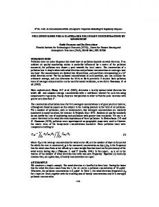
A preliminary international classification of organic matter was discussed during a workshop on “Organic Matter Classification” in Amsterdam (Lorente & Ran 1991). In this workshop the organic matter was designated Palynological Organic Matter (POM). The POM was divided into four major groups: palynomorphs, structured debris, amorphous matter and indeterminate matter. These were then subdivided into several categories. In the first monographic work on palynofacies Tyson (1995) revised (and reevaluated) the palynofacies terms. This author presented an informal classification (Tyson, 1995, p.350) close to the proposal presented in the workshop in Amsterdam. This classification is used herein (Figures 3.2-3.4) and kerogen categories are illustrated in Figure 3.5.

3.2.4.2 Kerogen categories

Amorphous Organic Matter (AOM) group

According to Tyson (1995) the AOM group consists of structureless particles that are observed under light microscopy. This group is composed of ‘AOM‘ and resin. The characteristics of the two subgroups are shown in Figure 3.2.

AOM Group

Origin

Description

"AOM"

Derived from phytoplankton or degradation of bacteria.

Structureless material. Color: yellow-orange-red; orange-brown; grey. Heterogeneity: homogeneous; with "speckles"; clotted; with inclusions (palynomorphs, phytoclasts, pyrite. Form: flat; irregular; angular; pelletal (rounded eleongate/oval shape).

Resin

Derived from higher plants of tropical and subtropical forest.

Structureless particle, hyaline, homogeneous, non-fluorescent, rounded, sharp to diffuse outline.

Figure 3.2. Classification of the amorphous organic matter (AOM) group used in this study (based on Tyson, 1995).

Phytoclast group

The phytoclast group consists of structured particles. This group is subdivided into two major subgroups: opaque and translucent. The opaque subgroup is subdivided into opaque-

17 equidimensional (O-Eq) and opaque-lath (O-La). The translucent subgroup is subdivided into fungal hyphae (Fh), wood tracheid with visible pits (Wp), wood tracheid without visible pits (Ww), cuticles (Cu) and membranes (Mb) (Figure 3.3).

Zooclast group

The zooclast group consists of animal-derived fragments. According to Tyson (1995) most zooclast fragments include arthropod exoskeletal debris, organic linings from bivalve shells and ostracode carapaces.

Opaque

Phytoclast Group

Description

Equidimensional (O-Eq)

Black particle from wood material. Long axis less than twice the short axis. Without internal biostructures.

Lath (O-La)

Black particle from wood material. Long axis more than twice the short axis. Without internal biostructures.

Wood tracheid with pits (Wp)

Translucent

Origin

Derived from the lignocellulosic tissues of terrestrial higher plants or fungi.

Brown particle from wood tracheid with visible pits.

Wood tracheid without pits (Ww)

Brown particle from wood tracheid without visible pits.

Cuticle (Cu)

Thin cellular sheets, epidermal tissue, in some case with visible stomates

Membranes (Mb)

Thin, non-cellular, transparent sheets of probable plant origin.

Fungal hyphae (Fh)

Derived from fungi

Individual filaments of mycelium of vegetative phase of eumycote fungi.

Figure 3.3. Classification of the phytoclast group used in this study (based on Tyson 1995).

Palynomorph group

The palynomorph group is subdivided into the sporomorph subgroup (Sm), which is further subdivided in spores and pollen grains; the phytoplankton subgroup (Pl), which consists of organic-walled microplankton and the zoomorph subgroup, composed of foraminiferal test linings (FTL) and scolecodonts (Figure 3.4). 3.2.4.3 Kerogen count

For a detailed paleoenvironmental study based on palynofacies, a count of the kerogen found in the slides is necessary. This count is presented as percentage (Appendix 3). According to Tyson (1995), the ideal count is 500 particles per sample using transmitted light microscopy.

18 In this study a total of 284 samples (117 samples from GTP-17-SE and 165 from GTP-24-SE) were studied. In each sample 500 particles were counted using transmitted light microscopy.

Palynomorph group

Terrestrial palynomorph produced by pteridophyte plants and fungi.

Pollen grains

Terrestrial palynomorph produced by Gymnosperm and Angiosperm plants.

*Palynomorphs with complex to simple morphology; usually spherical to subspherical shapes; with several ornamentation types; apertures may be present.

Foraminiferal test linings

Organic linings of benthic foraminifera.

Chitinous linings; brown coloured; inner smaller chambers often darker.

Sporomorph subgroup

parts of some polychaete Scolecodonts Mouth worms (mostly marine).

Acritarchs

Small microfossils of unknown and probably varied biological affinities.

cysts produced during Dinoflagellate Resting the sexual part of the life cycle of cysts Class Dinophyceae survives.

Phytoplankton subgroup

Description Triangular or circular palynomoph; Trilete spore with 3 laesurae (Y-mark); Monolete spore single laesura; varied ornamentation

Spores

Zoomorph subgroup

Origin

Fossilising structures produced

Prasinophytes by small quadriflagellate algae (Division Pyrrhophyta).

colonial freshwater Chlorococcale Exclusively algae (Botriococcus and algae Pediastrum)

Chitinous tooth-like jaw, dark brown; size 100-1000 µm. Central cavity enclosed by a wall of single or multiple layers; fossils with various form and sculpturing, ranging from types resembling dinoflagellates to those resembling chitinozoans; Size 5-240 µm Main feature is the paratabulation which divides the theca and cyst in rectangular or polygonal plates separated by sutures; 3 main morphologies: proximate, cavate and chorate; often with an opening (arceopyle) through which excystment occurs.

Most, like Tasmanites, are spherical; diameter 50 to 2000 µm, smooth and thick-walled. Botriococcus: irregular globular colonies; size 30 to 2.000 µm, sometimes with several lobes; orangebrown. Pediastrum: radially-symmetrical colonial green algae; mostly 30-200 µm in diameter and with one or two horns on the outermost ring of cells. Inner cells may be irregularly-shaped with spaces between cells, or closely packed.

Figure 3.4. Classification of the palynomorph group used in this study (based on Tyson, 1995).

3.2.4.4 Kerogen distribution

In marine environments the proximal-distal trend is one of the most important controls on kerogen distribution. For a detailed marine environmental analyses several kerogen distribution trends and parameters have been used (cf. Tyson, 1993, 1995) (Figure 3.6). These trends and parameters are based on percentages of kerogen categories.

2 3 1

B A

4 5

6

9 7

8

30µm

Figure 3.5. Kerogen categories. 1) AOM; 2) Resin (Re); 3) Wood tracheid without pits (Ww); 4) A- opaque lath (O-La), Bopaque equidimensional (O-Eq); 5) Wood tracheid with pits (Wp); 6) Fungal hyphae (Fh); 7) Membrane (Mb); 8) Cuticle; 9) Zooclast.

20 3.2.4.5 Kerogen trends

Percentage of ‘AOM‘ (of total kerogens)

A large amount of ‘AOM‘ results from a combination of high preservation rate and lowenergy environments. The preservation of ‘AOM‘ is directly related to dysoxic conditions and consequently, but not necessarily, correlated to high primary productivity (Tyson, 1993). According to Tyson (1993) in carbonate facies the ‘AOM’ may be the only kerogen available for preservation. Percentage of phytoclasts (of total kerogens)

High percentages of components the phytoclast group are mostly related to proximal depositional conditions. The main controlling factor is the short transport of the particles. Other factors, such as oxidizing conditions and the relative resistance of lining tissues are also associated with the proximity of the source area (Mendonça Filho, 1999). Generally, large amounts of phytoclast particles are deposited by rivers in estuaries and delta environments, both close to shorelines. However, deposition also occurs in deep waters, by turbidity currents (Habib, 1982).

Parameters

Environmental factors Proximal-distal trend

Distal anoxic facies

Upwelling (with arid hinterland)

% phytoclast/kerogen % AOM/kerogen % palynomorph/kerogen

?

Opaque : translucent phytoclasts

?

% cuticle/ phytoclasts

negligible

% sporomorphs/palynomorphs Frequency of tetrads

?

% microplankton/palynomorphs Peridinoid : gonyulacoid dinocysts

?

Dinocyst species diversity Absolute dinocyst abundance Frequency of foraminiferal lining high-low low-high

high-low-high low-high-low

decreases increases

may increase may decrease

Figure 3.6. Some parameters used in palynofacies analysis (adapted from Tyson 1995).

? ?

21 Percentage of palynomorphs (of total kerogens)

The palynomorph group is the least abundant of the three main groups, therefore its occurrence is controlled by ‘AOM‘ and phytoclast dilution (Tyson, 1993). Large amounts of palynomorphs, dominated by sporomorphs, indicate proximity of terrestrial sources associated with oxygenated environments. Consequently, a small amount of ‘AOM‘ is observed as a result of low preservation rates. With moderate proximity to land large amounts of palynomorphs can also be found, although without dilution of phytoclasts (Tyson, 1995). If microplankton dominates the palynomorph group, the environment may be of a distal shelf, with adjacent land areas being generally arid, oxygenated and with low ‘AOM‘ preservation but high productivity. The abundance of microplankton is inversely related to that of the sporomorphs (Tyson, 1993). Depending on the type of microplankton the ratio of sporomorphs to phytoplankton reflects the proximal-distal trend. The ratio of peridionioid to gonyaulacoid dinocysts (P/G ratio) also reflects the nearshore-offshore trend (see Chapter 7).

3.2.4.6 Ratios and Parameters

The palynofacies parameters and ratios used herein follow Tyson (1995). He suggested that for the ratios the sum of the two components must to be at least 50 particles. The ratios of opaque to translucent phytoclasts (O:TR) and of equidimensional to lath (O-Eq:O-La) opaque phytoclasts should be plotted as log graphs, because the values give more symmetrical plots (Tyson, 1995). For the palynomorph parameters the tetrad abundances and PMI values were employed.

Ratio of opaque to translucent phytoclasts (O:TR)

According to Tyson (1993) opaque phytoclast particles derive mainly from oxidation of translucent material, which has been transported over a prolonged period of time. In contrast, translucent particles are deposited in nearshore environments without a prolonged transport. Therefore, the ratio between these two categories could indicate the proximal-distal trend.

22 Ratio of equidimensional to lath opaque phytoclast (O-Eq:O-La)

This ratio also indicates a proximal-distal trend. A large amount of equidimensional particles suggests close proximity as a result of short transport. These equidimensional particles are sorted according to their buoyancy, where smaller particles are deposited in distal environments (Steffen & Gorin, 1993a). This interpretation is applied especially when the equidimensional particles are larger than the lath ones.

Abundance of tetrads

Tetrads consist of clusters of four pollen grains or spores. High amounts of tetrads indicate short duration of transport and consequently deposition in nearshore environments. Theoretically, a prolonged transport would cause disaggregation of the tetrads. However, tetrads are also found in deep water, especially when the pollen grains are small (for example Classopollis). Clusters of more than four pollen grains can also be found, sometimes containing up to 15 grains or more. These aggregates clearly indicate a short transport from their place of origin.

Palynologycal Marine Index (PMI)

As the PMI is based on the palynomorph diversity of terrestrial and marine palynomorphs; therefore, it was used as a substitute for terrestrial:marine ratio. The application of PMI has already been described.

3.2.4.7 Influence of lithology on kerogen groups

The relationship between lithology and kerogen distribution has been discussed by Tyson (1995), Mendonça Filho (1999), and Piper (1996), among others. According to Piper (1996) the sediment grain size influences the distribution of kerogen because of hydrodynamic equivalence or post-depositional oxidation. Changes in kerogen distribution due to environmental variations may be confused with changes of lithology, making it important to identify and separate these lithological influences on kerogen distribution. To this end Tyson (1995) suggested a comparison of samples with similar granulometric composition. The lithological data is best evaluated at two levels of scale: first the lithology of each sample and

23 then the dominant lithology of the interval where this sample was taken. This detailed lithological investigation suggested by Tyson (1995) is applied herein (Appendix 1).

3.2.5 Geochemical analysis

The geochemical study was based on a total of 140 samples from well GTP-24-SE processed for geochemical analyses in the Geochemistry Section of Petrobras, Rio de Janeiro, Brazil. The geochemical methods employed in this study included Total Organic Carbon (TOC) determination, Rock-Eval pyrolysis and fluorescence. The accumulation of organic matter (OM) in sediments is estimated using TOC analysis. According to Tyson (1995) TOC analysis is a convenient method to determine the abundance of OM in sediments. The accumulation of OM is controlled by major factors such as primary productivity, water depth, and sediment grain size. The TOC is always controlled by three main variables: input of organic matter (OM), preservation of the supplied OM, and dilution of the OM by sediment accumulation (Tyson, 1995). The results of the TOC and sediment grain size analyses are presented here. The values of TOC in marine rocks range from ca. 0.1% (deep-sea pelagic deposits) to 94% (coals) (Tyson, 1995). Rock-Eval pyrolysis involves the measurement of parameters such as hydrogen and oxygen indices, (HI) and (OI), respectively, S1 (free hydrocarbons), S2 (residual petroleum potential), S3 (generate CO2), and Tmax (temperature of maximum hydrocarbon evolution from kerogen, oC). These parameters are useful to characterize the organic matter and source rock potential. For this study only the HI (measured in units of mg hydrocarbon/g total organic carbon, mgHC/gTOC) and OI (measured in units of mgCO2/gTOC) (Miles, 1989) indices were used. The diagram HI versus OI, also known as a "modified van Klevelen diagram", was employed to characterize the organic matter type. This characterization is based on four kerogen types that are based purely on chemical composition of the kerogen; i.e. on the C, H and O content (Miles, 1989) and identified in the diagram (Table 3.2). In fact, these four kerogen types are based only on the hydrogen content and not on morphology. Types I and II are characterized by well-preserved AOM and Types III and IV by woody material (phytoclasts).

24 Table 3.2. Kerogen types. Data from Tyson 1995 and Miles 1989. Kerogen Type

Main environment

Origin

I

algal or cynobacterial materials

Anaerobic, in particular lacustrine

II

mixture of phytoplankton, zooplankton and bacterial material

Anaerobic to dysaerobic, marine

III

predominantly contiental plants and vegetal debris

Oxic, marine, deltaic

IV

continental plants

Oxidized in subaerial environments and/or recycled from older sediments

A total of 164 samples were analyzed to estimate the fluorescence parameters. This parameter, based on the qualitative preservation scale of Tyson (1995, p. 347) (Figure 3.7), was used to estimate the thermal maturity. The different fluorescence colors are indicative of the level of maturity of the organic matter. This (kerogen) shows autofluorescence when excited by ultra-violet (UV) light through a fluorescence microscopy. According to Bordenave (1993), the fluorescence is caused by the emission of photons by fluorophores when excited by electromagnetic radiation.

Characteristics of organic matter under fluorescence 1

Kerogen is all non-fluorescent (except perhaps for rare fluorescent palynomorphs, such as algae, or cuticles). 1a. AOM very rare (50% of TK

30-50% of TK

10-30% of TK

5-10% of TK

AOM Group

Cluster

Kerogen groups

A1

Phytoclasts/ AOM

A2

Phytoclasts/ Palynomorphs

A3

Phytoclasts

A2

Phytoclasts/ Palynomorphs

B1

AOM

B2

AOM/ Palynomorphs

Supercluster

Supercluster A

sample (m)

50

0.4-5% of TK

Supercluster B

Linkage Distance 60

Sporomorph Group

Q-mode

Phytoclast Group

R-mode

absent TK - total kerogen

Figure 8.2. Dendrograms by r and q-mode of well GTP-17-SE showing the grouping of samples (q-mode) and kerogen groups (r-mode).

20

10

0

sample (m) 12.64 49.7 97.65 339.3 313.25 237.7 357.5 295.1 98.2 146.1 157.15 189.8 291.5 289.6 217 224.6 272.55 109.4 124.67 178.56 211.85 112.7 304.05 342.05 46.35 51.8 101.7 91.25 60.7 130.55 170.43 309.53 331.3 308.95 135.75 384.6 322.25 13.25 16.65 22.88 80.4 83 299.3 268.75 122.85 227.7 18.63 99.2 20.85 134.45 200.68 208.3 241.25 403.75 26.83 72.25 50.6 160.35 252.6 19.24 19.35 62.25 25.3 327.43 349.18 28 120.6 37.55 86.7 377.65 124.4 42.65 128.1 214.75 268.05 33.2 119.5 336.2 88.4 222 103.15 222.25 167.25 32.25 227.1 240.65 249.1 247 64.65 256.1 110.6 243.95 382.75 190.75 237.6 239.75 15.55 364.9 67 15.78 17.9 22.8 67.4 262.95 393.05 398.05 39.45 82.55 57.8 59.3 35.95 255.65 318.65 337.6 268.3 42.25 182.6 56.95 66.45 71.66 77.2 75.4 57.6 318 35.1 326.45 367.65 16 58.7 400.53 54.5 19.85 52.35 254.6 259.05 409.9 23.55 300.6 20.53 44.15 24.05 47.9 205.85 30.6 40.1 182.06 414.95 16.45 94.35 277.7 26.23 56.1 202.37 48.6 258.5 84.9 108.1 265.1 232.9

>50% of TK

30-50% of TK

10-30% of TK

5-10% of TK

AOM Group Cluster

Kerogen groups

A

Phytoclasts

B1

B2

Phytoclasts/ AOM

Phytoclasts/ Palynomorphs

C

Palynomorphs

D1

AOM

AOM/ Palynomorphs

D2

0.4-5% of TK

Superluster

Supercluster A

30

Supercluster B

40

Supercluster C

50

Supercluster D

60

Sporomorph Group

Q-mode Linkage Distance

Phytoclast Group

R-mode

absent TK - total kerogen

Figure 8.3. Dendrograms by r and q-mode of well GTP-24-SE showing the grouping of samples (q-mode) and kerogen groups (r-mode).

82 In this well the main break separates clearly the samples with high abundances of the AOM group from those with high abundances of phytoclasts (r-mode) (Figure 8.3). Based on the palynofacies composition, their abundance and the clusters, the types were grouped into nine palynofacies associations (Figure 8.4), which were used for the definition of palynofacies units Palynofacies associations Phy-o Phy-o/Pal-s Phy-o/Pal-mp Phy-o/AOM

Pal-s/Phy-o

Pal-mp/Phy-o

Description Predominance of the phytoclast group with a high content of opaque particles. Predominance of the phytoclast group with a high content of opaque particles combined with sporomorphs. Predominance of the phytoclast group with a high content of opaque particles combined with marine palynomorphs. Predominance of the phytoclast group with a high content of opaque particles combined moderate content of the AOM group. Predominance of the palynomorph group with a high content of sporomorphs combined with opaque particles. Predominance of the palynomorph group with a high content of marine palynomorphs combined with opaque particles.

AOM/Phy-o

Predominance of the AOM group combined with opaque particles.

AOM/Pal-s

Predominance of the AOM group combined with sporomorphs.

Predominance of the AOM group combined with marine palynomorphs. Figure 8.4. Palynofacies associations identified after the cluster analyses. AOM/Pal-mp

8.2 Palynofacies units

The pattern of stratigraphic distribution of the palynofacies associations forms the base for the definition of palynofacies units. The variations reflect from environmental changes, mainly shoreline shifts that influenced the proximal-distal trend. The palynofacies units were defined according to Brugman et al. (1994), who established units and subunits to Lettenkeuper of the Germanic Basin, based on quantitative data on total organic matter. They indicated that the stratigraphical subdivisions of the succession based on ecophases may allow interpretations of depositional environments, but at some intervals because of the lack of significant palynomorphs, the palynofacies units are very useful to interpret the paleoenvironments.

83 8.2.1 Palynofacies units of well GTP-17-SE

The sedimentary succession of GTP-17-SE is represented by a lower part characterized by moderate to high contents of ‘AOM‘ kerogen and an upper part with high to very high amounts of the phytoclast group. There is a progressive increase in phytoclast particles upward, in particular of opaque particles. The mean of entire succession (in this study used as general mean) of the kerogen categories is displayed in Figure 8.5. The succession of GTP17-SE was subdivided into eight units (units A-17 to H-17) as illustrated in Figure 8.22. Phytoclast Group

Kerogen groups Opaque

Max. Min. General mean

Palynomorph Group

Translucent

Marine

AOM %

Ph%

Pa %

Zoocl %

O-Eq

O-La

Fh

Wp

Cu

Ww

Mb

74.2

100

49.2

2.0

53.5

89.3

2.6

4.4

24.7

59.8

1.4

Ftl

Df

65.1 71.1

Terrestrial Fwp 0.6

-

11.2

-

-

-

32.4

-

-

-

0.5

-

-

-

-

10.9

73.7

15.2

0.3

12.5

59.4

0.2

0.7

3.3

23.8

0.1

2.8

4.5

0.02

Pl

Sp

100 36.0 24.6

-

85.9 6.8

Figure 8.5. Palynofacies summary for well GTP-17-SE. Relative abundance (%) of kerogen groups from total of kerogen. Relative abundance (%) of the phytoclast group from total phytoclasts. Relative abundance (%) of the palynomorph group from total palynomorphs. AOM= amorphous organic matter; Ph= phytoclast; Pa= palynomorphs; Zoocl= zooclast; O-Eq= opaque equidimensional; O-La= opaque lath; Fh= fungal hyphae; Wp= wood tracheid with pits; Ww= wood tracheid without pits; Mb= membrane; FTL= foraminiferal test linings; Df= dinoflagellates; Pl= pollen; Sp= spores.

The values of the ratios of opaque to translucent (O:TR) for GTP-17-SE range from –0.27 to 1.9, with a mean of 0.47 (Table 8.1). The ratio curve is characterized by a slight long-term increasing trend upwards. The ratios of equidimensional to lath particles (O-Eq:O-La) range from 0.07 to –1.85 (mean = -0.79) and the ratio curve shows a marked increase upwards. The abundance of tetrads shows a slight decrease upward. The abundance values range from 0 to 23.5% (% of palynomorphs) with a general mean of 3.8%. The PMI values range from 100.00 (nonmarine palynomorphs) to 200.00, with a mean of 122.90. The results found in each unit are shown throughout this well section and the stratigraphic distribution of the palynofacies ratios and parameters are illustrated in Figure 8.23. Table 8.1. Summary of palynofacies parameters of well GTP-17-SE. O= opaque; TR= translucent; O-Eq= opaque equidimensional; O-La= opaque lath. O:TR ratio (log10)

O-Eq:O-La ratio (log10)

Tetrad frequency (%)

PMI

Max.

1.90

0.10

23.50 -

200.00

Min.

-0.26

-1.90

0.47

-0.79

General mean

100.00 3.80

122.90

GTP-17-SE

middle? Albian

60

80

0

10

30

50

0

20

40

60

80

0

40

10

Wp % 0

20

Fh %

10

Cu % 0

10

Ww % 30

0

10

30

Zoo %

Mb % 50

0

0

O-La %

O-E %

10

0

AOM %

Palynomorph zones

10

Sm % 0

20

FTL % 40

0

LithoAge stratigraphy

Ph % 20

0

10

50

Units 30

Unit H-17

Classopollis echinatus

Unit G-17 Angico Member

Riachuelo Formation

100

150

200

Unit F-17 Equisetosporites maculosus

upper Aptian

250

Unit E-17 300

Oiteirinhos Member Ibura Member

Muribeca Formation

Unit D-17

350

Unit C-17

Unit B-17 400

Sergipea variverrucata

Unit A-17 450

Figure 8.22. Stratigraphic distribution of kerogen categories in well GTP-17-SE. AOM= amophous organic matter; O-Eq= opaque equidimensional; O-La= opaque lath; Fh= fungal hyphae; Wp= wood tracheid with pits; Ww=wood tracheid without pits; Cu= cuticle; Mb= membrane; Zoo= zooclast; Sm= sporomorphs; FTL= foraminiferal test linings; Ph= phytoplankton.

GTP-17-SE LithoAge stratigraphy

O:TR

Palynomorph zones

-0.5

O-Eq:O-La 2

-2

Tetrads 0.5

0

PMI 25

100

225

Palynofacies units

Inferred proximal-distal trend p d

middle? Albian

0

Unit H-17

50

Classopollis echinatus

Unit G-17 Angico Member

Riachuelo Formation

100

150

200

Unit F-17

Equisetosporites maculosus

upper Aptian

250

Unit E-17 300

Oiteirinhos Member Ibura Member

Muribeca Formation

Unit D-17 Unit C-17

350

Unit B-17 400

Sergipea variverrucata

Unit A-17

450

500

0.47

-0.79

3.8

122.9

Figure 8.23. Stratigraphic distribution of the palynofacies ratios and parameters of well GTP-17-SE. Abbreviation see Table 8.2.

Trendline General mean

p= proximal d= distal

86 Unit A-17 (471-393 m) - Palynofacies association AOM/Pal-s

This unit is characterized by relatively large amounts of the AOM group, which are combined with a moderate abundance of terrestrial palynomorphs (sporomorph subgroup). However, marine palynomorphs, in particular foraminiferal test linings (FTL), are present. Despite the large amount of phytoclasts, this unit is characterized by the AOM group because its average abundance (32.3%) in this unit is much higher than its general mean (10.9%) (see Figure 8.6). The AOM group reaches high values (up 70% of total kerogen). Its abundances decrease towards the top, where they make up only 0.4% of the kerogen. The phytoclast group contains mainly opaque-lath particles. The trendline of this group decreases upwards. Translucent particles are present in moderate amounts throughout the succession.

Phytoclast Group

Kerogen groups Opaque

Unit A-17 (AOM/ Pal-s)

Palynomorph Group Marine

Translucent

Terrestrial

AOM %

Ph%

Pa %

Zoocl %

O-Eq

O-La

Fh

Wp

Cu

Ww

Mb

Ftl

Df

Fwp

Max.

74.2

89.4

29.3

1.2

25.1

89.3

-

3.3

3.3

31.1

-

65.1

1.0

0.5

97.5 7.0

Min.

0.4

11.2

10.0

-

-

54.5

-

-

-

10.3

-

-

-

-

32.5 1.5

69.1

-

0.7

0.9

18.1

-

11.6

0.3

0.1

84.0 4.2

59.4

0.2

3.3

23.8

0.1

0.1

2.8

4.5

0.02

85.9 6.8

Mean

General mean

32.3

51.1

16.5

0.2

11.1

10.9

73.7

15.2

0.3

12.5

Pl

Sp

Figure 8.6. Percentage mean values of the kerogen categories for Unit A-17. Relative abundances and abbreviations as in Figure 8.5.

Ratios and parameters. The average values of the O:TR ratio are higher than the general mean (Figure 8.7). The ratio curve shows a constant trendline (Figure 8.23). The O-Eq:O-La shows a strong fluctuation; however, the trendline shows a slight decreasing trend indicating an increase of O-La upwards. The tetrad abundances show the highest values found in this well (23.5%), with a marked increasing trend upwards. The unit is characterized by moderate to high PMI values. The PMI curve also increases upwards; however, in the uppermost sample no marine palynomorphs were observed (Figure 8.23).

Ratios and Parameters

Max.

Min.

Unit Mean

General mean

Trendline

O:TR ratio (log10)

0.92

0.25

0.64

0.47

constant

O-Eq:O-La ratio (log10)

0

-1.85

-0.77

-0.79

slightly decrease upwards

Tetrad abundance (%)

23.50

-

5.90

3.80

increase upwards

119.4

122.9

increase upwards

PMI

150.00 100.00

Remarks

highest value

Figure 8.7. Summary of palynofacies ratios and parameters of Unit A-17. For abbreviations see Table 8.1.

87 Unit B-17 (393-374 m) - Palynofacies association Phy-o/Pal-s Unit B-17 is strongly dominated by opaque phytoclasts, which are associated with moderate to high contents of terrestrial palynomorphs (Figure 8.8). The phytoclast group is composed mainly of opaque-lath particles. Translucent particles are mainly composed of Ww particles. The palynomorph group in this unit contains mainly terrestrial palynomorphs, particularly pollen grains. The marine palynomorphs are represented by only two forms (FTL and dinocysts). The AOM occur in low to moderate abundances increasing gradually within the uppermost part of the unit. Phytoclast Group

Kerogen groups Opaque

Palynomorph Group

Translucent

Marine

Terrestrial

AOM %

Ph%

Pa %

Zoocl %

O-Eq

O-La

Fh

Wp

Cu

Ww

Mb

Ftl

Df

Fwp

Pl

Sp

38.0

87.2

23.0

0.2

20.7

87.8

1.0

1.3

5.3

34.9

0.5

0.5

0.5

-

99.0 5.0

Unit B-17

Max. Min.

1.0

44.2

10.0

-

2.1

57.3

-

-

-

9.0

-

-

-

-

95.0 1.0

(Phy-o/ Pal-mp)

Mean

15.3

67.9

16.9

0.1

7.7

66.6

0.3

0.5

1.9

22.8

0.1

0.1

0.1

-

97.3 2.5

10.9

73.7

15.2

0.3

12.5

59.4

0.2

0.7

3.3

23.8

0.1

2.8

4.5

0.02

85.9 6.8

General mean

Figure 8.8. Percentage mean values of the kerogen categories for Unit B-17. Relative abundances and abbreviations as in Figure 8.5.

Ratios and parameters. The ratio curve of O:TR shows a decreasing trend upwards. The mean value is higher than the general average (Figure 8.9). The O-Eq:O-La ratio clearly shows an increasing trend, due to the progressive increase of equidimensional particles. The tetrad abundances show low to moderate values, with a slight increasing trend upwards (Figure 8.23). The unit is characterized by low PMI values; marine palynomorphs are present only in two samples.

Ratios and Parameters

Max.

Min.

Unit Mean

General mean

Trendline

O:TR ratio (log10)

0.98

0.23

0.49

0.47

decrease upwards

O-Eq:O-La ratio (log10)

-0.70

-1.50

-1.10

-0.79

increase upwards

Tetrad abundance (%)

4.00

0.50

2.60

3.80

constant

PMI

150.00

100.00

119.40

122.90

constant

Figure 8.9. Summary of palynofacies ratios and parameters of Unit B-17. For abbreviations see Table 8.1.

Unit C-17 (374-325 m) - Palynofacies association AOM/Pal-s Unit C-17 shows the same characteristics as Unit A-17, in which a high relative abundance of the AOM group (Figure 8.10) is observed. The palynomorphs are composed mainly of

88 terrestrial palynomorphs; however at 328.67 the marine palynomorphs show a major peak in abundance due to the high relative abundances of FTL and the genus Spiniferites. The phytoclast group is also present in moderate to high abundances (Figure 8.10). This group is composed mainly of O-La particles. The translucent particles are predominately composed of Ww particles, which show moderate to high values (Figure 8.10). Phytoclast Group

Kerogen groups Opaque

Unit C-17 (AOM/ Pal-s)

Palynomorph Group

Translucent

Marine

Terrestrial

AOM %

Ph%

Pa %

Zoocl %

O-Eq

O-La

Fh

Wp

Cu

Ww

Mb

Ftl

Df

Fwp

Pl

Sp

Max.

67.2

73.4

30.2

1.2

8.6

86.5

1.1

4.4

5.7

59.8

1.2

13.5

9.5

-

100

8.5

Min.

13.6

14.0

10.0

-

2.7

34.6

-

-

-

9.9

-

-

-

-

75.5

-

Mean

35.0

50.4

14.3

0.3

4.7

64.9

0.3

0.8

1.9

27.3

0.2

2.4

1.1

-

94.1 2.4

10.9

73.7

15.2

0.3

12.5

59.4

0.2

0.7

3.3

23.8

0.1

2.8

4.5

0.02

85.9 6.8

General mean

Figure 8.10. Percentage mean values of the kerogen categories for Unit C-17. Relative abundances and abbreviations as in Figure 8.5.

Ratios and parameters. The O:TR ratio in Unit C-17 is characterized by strong fluctuations; however, the ratio curve shows a clear decrease upward reflecting an increase in translucent particles (Figure 8.11). The average value (0.39) is lower than the general mean (Figure 8.11). The O-Eq:O-La ratio also shows strong fluctuations, but the ratio curve increases slightly upward due to an increase in equidimensional particles. Tetrad abundances range from 0 to 10%, and its trendline is constant. Unit C-17 is characterized by the highest PMI value (200.00) of the entire succession. The PMI values increase markedly in the upper part of the unit (Figure 8.23).

Ratios and Parameters

Max.

Min.

Unit Mean

General mean

Trendline

O:TR ratio (log10)

0.92

-0.21

0.39

0.47

decrease upwards

O-Eq:O-La ratio (log10)

-0.83

-1.50

-1.14

-0.79

increase upwards

Tetrad abundance (%)

10.00

-

4.50

3.80

slightly decrease upwards

PMI

200.00

100.00

116.20

122.90

increase upwards

Figure 8.11. Summary of palynofacies ratios and parameters of Unit C-17. For abbreviations see Table 8.1.

Unit D-17 (325-300 m) - Palynofacies association Phy-o-t

Unit D-17 is strongly dominated by the phytoclast group. The abundance difference between the subgroups (opaque and translucent) is very small; therefore, this unit was named Phy-o-t. The O-La (opaque) and Ww (translucent) are the most abundant particles; however, the cuticle fragments show a marked increase. The AOM group shows very low to high abundances, though, the average abundance is low. The palynomorphs are dominated by

89 pollen grains. The spores show low to moderate abundances. The marine palynomorphs are mainly represented by rare dinocysts (Figure 8.12). Phytoclast Group

Kerogen groups Opaque

Palynomorph Group

Translucent

Marine

Terrestrial

AOM %

Ph%

Pa %

Zoocl %

O-Eq

O-La

Fh

Wp

Cu

Ww

Mb

Ftl

Df

Fwp

Max.

43.8

88.6

20.6

0.8

16.6

64.2

0.7

1.7

7.2

45.8

0.9

3.5

5.5

0.6

98.5 4.5

Min.

0.4

35.2

9.6

0.4

5

41.2

-

0.2

0.6

22.4

-

-

-

-

91.0 1.0

(Phy-o-t) Mean

6.1

79.1

14.2

0.6

9.6

52.6

0.4

0.9

3.7

32.6

0.2

1.4

1.8

0.1

94.4 2.2

General mean

10.9

73.7

15.2

0.3

12.5

59.4

0.2

0.7

3.3

23.8

0.1

2.8

4.5

0.02

85.9 6.8

Unit D-17

Pl

Sp

Figure 8.12. Percentage mean values of the kerogen categories for Unit D-17. Relative abundances and abbreviations as in Figure 8.5.

Ratios and parameters. All O:TR values are lower than the general average (0.47) (Figure 8.13). The trendline is constant reflecting the stable amount of translucent particles in this unit (Figure 8.23). The O-Eq:O-La curve shows a gradual increase upward. Like the other ratio, the average value (-0.77) is lower than the general mean. The abundances of tetrads show a slightly increase towards the top. In this unit the PMI values are moderate to high and the trendline shows an increase upwards (Figure 8.23).

Ratios and Parameters

Max.

Min.

Unit Mean

General mean

Trendline

O:TR ratio (log10)

0.46

0.03

0.22

0.47

constant

O-Eq:O-La ratio (log10)

-0.51

-1.00

-0.77

-0.79

slightly decrease upwards

Tetrad abundance (%)

9.50

-

3.10

3.80

decrease upwards

PMI

160.00

100.00

130.70

122.90

slightly increase upwards

Figure 8.13. Summary of palynofacies ratios and parameters of Unit D-17. For abbreviations see Table 8.1.

Unit E-17 (300-277 m) - Palynofacies association Pal-mp/Phy-o-t

This unit is characterized by the relatively high abundances of marine palynomorphs, in particular dinocysts (Figure 8.14). This is combined with nearly equal amounts of opaque and translucent particles (phytoclast group), in which O-La and O-Eq of the opaque subgroup and Ww (translucent) are the most abundant. The AOM group reaches moderate values, and its abundance curve increases towards the top.

90 Phytoclast Group

Kerogen groups Opaque

Palynomorph Group

Translucent

Marine

Terrestrial

AOM %

Ph%

Pa %

Zoocl %

O-Eq

O-La

Fh

Wp

Cu

Ww

Mb

Ftl

Df

Fwp

Max.

25.8

86.2

28.8

0.8

26.2

59.4

0.3

1.2

3.5

51.4

0.3

3.5

28.5

-

Min.

0.4

54.8

12.0

-

4.1

40.7

-

0.3

0.9

19.9

-

0.5

0.5

-

69.5 1.5

(Pal-mp/ Phy-o-t) Mean

7.2

69.2

22.7

0.4

12.9

50.1

0.1

0.7

2.7

33.5

0.1

1.8

11.5

-

83.8 3.0

General mean

10.9

73.7

15.2

0.3

59.4

0.2

0.7

3.3

23.8

0.1

2.8

4.5

0.02

85.9 6.8

Unit E-17

12.5

Pl

Sp

95

6.0

Figure 8.14. Percentage mean values of the kerogen categories for Unit E-17. Relative abundances Relative abundances and abbreviations as in Figure 8.5.

Ratios and parameters. The average values of the O:TR ratio are lower than the general mean (0.47) due to the relatively large amounts of translucent particles. The ratio curve is characterized by a progressive decrease upwards (Figure 8.15). The abundance curve for the O-Eq:O-La ratio reflects the moderate to high abundance of the O-Eq particles; however, the abundance curve decreases upwards. The tetrad abundances show low to moderate values with a slight increasing trend upward. All values obtained for the tetrad abundance are lower than the general mean (Figure 8.15). Unit E-17 is characterized by moderate to high PMI values. The PMI curve shows a clear increase upwards.

Ratios and Parameters

Max.

Min.

Unit Mean

General mean

Trendline

O:TR ratio (log10)

0.50

-0.10

0.24

0.47

decrease upwards

O-Eq:O-La ratio (log10)

-0.21

-1.00

-0.69

-0.79

decrease upwards

Tetrad abundance (%)

3.00

-

0.90

3.80

slightly increase upwards

PMI

150.00

120.00

136.30

122.90

increase upwards

Figure 8.15. Summary of palynofacies ratios and parameters of Unit E-17. For abbreviations see Table 8.1.

Unit F-17 (277-143 m) - Palynofacies association Phy-o/Pal-s

Unit F-17 is strongly dominated by opaque phytoclasts combined with a moderate to high content of terrestrial palynomorphs (Figure 8.16) which characterize this unit. The phytoclast group is composed mainly of opaque-lath particles (O-La); however O-Eq shows the highest peak in abundance of this well. Translucent particles are mainly composed of Ww particles and cuticles that are common in this unit. The palynomorph group contains mainly terrestrial palynomorphs, in particular pollen grains. The marine palynomorphs are mainly represented by dinocysts. Generally, ‘AOM’ occurs in low abundances and decreases towards the top (Figure 8.22).

91 Phytoclast Group

Kerogen groups Opaque

Palynomorph Group

Translucent

Marine

Terrestrial

AOM %

Ph%

Pa %

Zoocl %

O-Eq

O-La

Fh

Wp

Cu

Ww

Mb

Ftl

Df

Fwp

Max.

17.4

99.3

35.6

1.8

53.5

74.7

2.6

2.4

19.1

51.4

1.4

6.5

13.0

-

Min.

-

64.2

0.7

-

2.0

36.3

-

0.3

0.3

0.5

-

-

-

-

(Phy-o/ Pal-s) Mean

1.9

82.4

15.5

-

12.6

54.5

0.3

0.8

4.3

27.5

0.2

0.9

2.0

-

88.4 8.7

General mean

10.9

73.7

15.2

0.2

12.5

59.4

0.2

0.7

3.3

23.8

0.1

2.8

4.5

0.02

85.9 6.8

Unit F-17

Pl

Sp

97.5 31.0 69

2.5

Figure 8.16. Percentage mean values of the kerogen categories for Unit F-17. Relative abundances Relative abundances and abbreviations as in Figure 8.5.

Ratios and parameters. The O:TR ratio shows a progressive increasing upwards indicated by a rise in opaque particles. In this unit the highest value of this ratio (1.9) is found; however, the average (0.39) is lower than the general mean value (0.47). The curve for the OEq:O-La ratio shows the same pattern as the O:TR. The curve for tetrad abundances shows strong fluctuations and a slight decrease upwards. The PMI curve also shows a strong fluctuations. In the upper part of the unit, two major peaks are recorded; however, the trendline shows a slight decrease towards the top (Figure 8.23).

Ratios and Parameters

Max.

Min.

Unit Mean

General mean

Trendline

O:TR ratio (log10)

1.90

-0.20

0.39

0.47

decrease upwards

O-Eq:O-La ratio (log10)

0.07

-1.50

-0.78

-0.79

decrease upwards

Tetrad abundance (%)

15.00

0.50

4.30

3.80

slightly increase upwards

120.50

122.90

increase upwards

PMI

162.50 100.00

Figure 8.17. Summary of palynofacies ratios and parameters of Unit F-17. For abbreviations see Table 8.1.

Unit G-17 (143-85 m) - Palynofacies association Pal-mp/Phy-o

This unit is characterized by the highest abundance of the palynomorph group, which is dominated by terrestrial elements. However, the percentages of these palynomorphs decrease upwards, whereas a clear increase in abundance of marine palynomorphs is observed. The high abundance of marine palynomorphs, in particular dinocysts (Figure 8.18), is characterized of this unit, as are high amounts of phytoclast particles. This group is composed mainly of opaque particles, in which O-La and O-Eq are the most abundant. The translucent particles are made up of moderate amounts of Ww and cuticle particles. The AOM group is rare, but increase in abundances upwards (Figure 8.22).

92 Phytoclast Group

Kerogen groups Opaque

Palynomorph Group

Translucent

Marine

Terrestrial

AOM %

Ph%

Pa %

Zoocl %

O-Eq

O-La

Fh

Wp

Cu

Ww

Max.

6.0

98.3

49.2

2.0

34.3

78.0

0.3

0.9

10.6

34.6

Min.

0.3

44.0

-

-

11.4

47.0

-

-

0.3

4.9

-

-

-

(Pal-mp/ Phy-o) Mean

2.7

75.5

21.2

0.6

20.2

57.5

0.1

0.5

2.8

19.1

12.5

5.6

0.1

66.6 15.3

General mean

10.9

73.7

15.2

0.3

12.5

59.4

0.2

0.7

3.3

23.8

2.8

4.5

0.02

85.9 6.8

Unit G-17

Mb

Ftl

Df

25.5 42.0

0.1

Fwp 0.5

Pl

Sp

94.5 36.0 36.8

5.0

Figure 8.18. Percentage mean values of the kerogen categories for Unit G-17. Relative abundances Relative abundances and abbreviations as in Figure 8.5.

Ratios and parameters. The average value (0.59) of the O:TR ratio is higher than the general mean value (Figure 8.19). The ratio curve shows a constant trendline (Figure 8.23). The O-Eq:O-La ratio is characterized by moderate to high values, in which the mean is lower than the general mean. The ratio curve shows a progressive decrease upwards. The tetrad abundances show a clear increase upward. The average abundance of the tetrads in this unit (4.6%) is higher than the general value (3.8%). The PMI values are moderate to high and the trendline indicates a slight increase upwards (Figure 8.23). The average (133.90) is higher than the general mean (Figure 8.45).

Ratios and Parameters

Max.

Min.

Unit Mean

General mean

Trendline

O:TR ratio (log10)

1.13

0.21

0.59

0.47

constant

O-Eq:O-La ratio (log10)

-0.16

-0.75

-0.48

-0.79

decrease upwards

Tetrad abundance (%)

11.00

0.50

4.60

3.80

increase upwards

PMI

160.00

100.00

133.90

122.90

slightly increase upwards

Figure 8.19. Summary of palynofacies ratios and parameters of Unit G-17. For abbreviations see Table 8.1.

Unit H-17 (85-18 m) - Palynofacies association Phy-o

Unit H-17 is strongly dominated by opaque phytoclasts reaching up to 100.0% of all kerogen categories. This group is composed mainly of O-La (Figure 8.20), but O-Eq particles are also present in large amounts. Translucent particles show moderate to high abundances and are mainly composed of Ww particles. The cuticle fragments show the highest value recorded in the well (see Figure 8.20). The unit is also characterized by extremely low abundances of the AOM group. The palynomorph group occurs in small to moderate amounts; however, despite of very high amounts of phytoclasts, the marine palynomorphs, in particular dinocysts, show the highest abundances in the whole section (Figure 8.20). The terrestrial palynomorphs show relatively low abundances. These elements are composed mainly of pollen grains; however, the spores show moderate to high abundances.

93 Phytoclast Group

Kerogen groups Opaque AOM %

Palynomorph Group

Translucent

Marine

Terrestrial

Ph%

Pa %

Zoocl %

O-Eq

O-La

Fh

Wp

Cu

Ww

Mb

Ftl

Df

Fwp

12.5 71.1

Pl

Sp

89

29.5

Unit H-17

Max.

3.2

100

15.3

1

38.1

79.8

0.2

1.2

24.7

40.1

0.2

Min.

-

81.4

-

-

2.8

32.4

-

-

-

2.2

-

-

-

-

24.6 2.6

(Phy-o)

Mean

1.5

91.3

7

0.2

19.6

61.5

0.03

0.4

4.4

14.1

0.02

3.1

20.7

-

66.5 9.7

General mean

10.9

73.7

15.2

0.3

12.5

59.4

0.2

0.7

3.3

23.8

0.1

2.8

4.5

-

0.02

85.9 6.8

Figure 8.20. Percentage mean values of the kerogen categories for Unit H-17. Relative abundances and abbreviations as in Figure 8.5.

Ratios and parameters. The curve for the O:TR ratio reflects the very large amounts of opaque particles. In spite of a strong fluctuations, the ratio curve shows a clear increasing trend. In the lower part of the curve there is an abrupt decrease (increase in translucent particles), where the lowest value of this ratio (-0.26) (Figure 8.21) is observed. The abundance curve for the O-Eq:O-La ratio reflects the moderate to high abundances of O-Eq particles. The tetrad abundance show very low to moderate values. The abundance curve shows a slight decreasing trend upwards (Figure 8.23). The PMI is characterized by a decrease in abundance upwards. In the abundance curve two parts can be distinguished: a lower part characterized by high PMI values, and an upper part marked by an abrupt decrease in PMI values (Figure 8.23).

Ratios and Parameters

Max.

Min.

Unit Mean

General mean

Trendline

Remarks lowest value

O:TR ratio (log10)

1.47

-0.26

0.70

0.47

increase upwards

O-Eq:O-La ratio (log10)

-0.17

-1.06

-0.61

-0.79

increase upwards

Tetrad abundance (%)

8.00

-

1.00

3.80

slightly increase upwards

140.60

122.90

decrease upwards

PMI

175.00 100.00

Figure 8.21. Summary of palynofacies ratios and parameters of Unit H-17. For abbreviations see Table 8.1.

8.2.2 Palynofacies units of GTP-24-SE

The succession of well GTP-24-SE is characterized by a long-term transgressive trend indicated by an increase of the AOM and palynomorph groups. This trend is best indicated by a progressive upward increase in marine palynomorph abundance, especially of dinocysts. The maximum, minimum and general means of kerogen categories for well GTP-24-SE are summarized in Figure 8.24. The sedimentary succession of GTP-24-SE was subdivided into ten units (Unit A-24-J-24) described below and illustrated in Figure 8.45.

GTP-24-SE LithoAge stratigraphy

Palynomorph zones

AOM % 0

10

20

30

40

O-Eq % 50

60

70

80

0

10

20

O-La % 30

0

10

20

30

40

Fh % 50

60

70

0

10

Wp % 0

10

Cu % 0

10

Ww % 0

10

20

30

40

50

Mb %

Zoo %

0

0

10

10

Sm % 0

10

20

30

FTL % 40

50

0

10

Ph % 20

0

10

20

Units 30

middle? Albian

0

Classopollis echinatus

Unit J-24 50

Taquari Member

Riachuelo Formation

Dejaxpollenites microfoveolatus 100

Unit I-24

150

Unit H-24

Equisetosporites maculosus

upper Aptian

200

Unit G-24

Unit F-24 250

Oiteirinhos Member

Sergipea variverrucata

Unit D-24 300

Unit C-24 350

Unit B-24 Ibura Member

Muribeca Formation

Unit E-24

400

Unit A-24

Figure 8.45. Stratigraphic distribution of kerogen categories in well GTP-24-SE. ‘AOM‘= amophous organic matter; Re= resin; O-Eq= opaque equidimensional; O-La= opaque lath; Fh= fungal hyphae; Wp= wood tracheid with pits; Ww=wood tracheid without pits; Cu= cuticle; Mb= membrane; Zoo= zooclast; Sm= sporomorphs; FTL= foraminiferal test linings; Ph= phytoplankton.

95 Phytoclast Group

Kerogen groups Opaque AOM %

Ph%

Max.

75.3

Min.

0.6 32.7

General mean

Palynomorph Group

Translucent

Marine

Pa %

Zoocl %

O-Eq

O-La

Fh

Wp

Cu

Ww

Mb

87.4

49

3.0

39.0

79.7

11.5

8.5

14.7

72.3

14.8 53.7 89.0

12.8

1.2

-

0.6

14.2

-

-

-

8.0

-

47.9

19.0

0.3

9.0

52.2

1.1

1.3

1.8

33.5

1.1

Ftl

-

Df

Terrestrial Fwp 1.5

-

7.8 24.9

0.1

Pl

Sp

100 32.5 4.0

-

61.0 6.3

Figure 8.24. Palynofacies summary for well GTP-24-SE. Relative abundances (%) of the kerogen groups from total kerogen. Relative abundances (%) of the phytoclast group from total phytoclasts. Relative abundances (%) of the palynomorph group from total palynomorphs. For abbreviations see Figure 8.5.

The highest and lowest values and means of entire succession of this well (general means) of the ratios and parameters of well GTP-24-SE are displayed in Table 8.2 and illustrate in Figure 46. The O:TR ratio curve is characterized by a slight long-term decreasing upward and the O-Eq:O-La ratio shows a clear increase towards the top. The curve of tetrad abundances is characterized by a slight long-term decrease upwards. The PMI curve is marked by a increase upwards reflecting the increase of marine palynomorphs.

Table 8.2. Summary of palynofacies parameters of well GTP-24-SE. For abbreviations see Table 8.1. O:TR ratio (log10)

O-Eq:O-La ratio (log10)

Tetrad frequency (%)

PMI

Max.

0.83

0.01

73.40

250.00

Min.

-0.53

-2.15

-

100.00

0.21

-0.84

5.90

138.90

General mean

GTP-24-SE LithoAge stratigraphy

O:TR

Palynomorph zones

-0.6

O-Eq:O-La 1.0

-2.5

Tetrads 0.5

0

PMI 80

100

Units 275

Inferred proximal-distal trend p d

middle? Albian

0

Classopollis echinatus

Unit J-24

50

Taquari Member

Riachuelo Formation

Dejaxpollenites microfoveolatus 100

Unit I-24

Equisetosporites maculosus 150

Unit H-24

Unit G-24

upper Aptian

200

Unit F-24 250

Oiteirinhos Member Ibura Member

Muribeca Formation

Unit E-24 Sergipea variverrucata

Unit D-24

300

Unit C-24 350

Unit B-24

400

Unit A-24

0.21

-0.84

5.9

Figure 8.46. Stratigraphic distribution of the palynofacies ratios and parameters of well GTP-24-SE. Abbreviation see Table 8.2.

138.9

Trendline General mean

p= proximal d= distal

97 Unit A-24 (415-383 m) - Palynofacies association AOM/Pal-s This unit is characterized by a high abundance of the AOM group combined with the palynomorph group that mainly consist of terrestrial elements, especially pollen grains (95.8% of sporomorph subgroup). Marine palynomorphs are relatively few and represented mainly by FTL. The phytoclast group is composed mainly of O-La particles, which show high abundances. Translucent particles are present but in moderate numbers. They are composed basically of Ww particles (Figure 8.25). Phytoclast Group

Kerogen groups Opaque

Unit A-24 (AOM/ Pal-s)

Palynomorph Group Marine

Translucent

AOM %

Ph%

Pa %

Zoocl %

O-Eq

O-La

Fh

Wp

Cu

Ww

Mb

Max.

65.0

51.7

17.8

1.6

12.3

70.4

1.6

2.0

0.6

28.3

-

Min.

32.3

18.8

11.4

-

4.3

65.7

-

-

-

17.1

-

-

-

Mean

49.0

35.1

15.2

0.6

8.2

67.6

0.6

0.2

0.2

22.3

-

7.5

32.7

47.9

19.0

0.3

9.0

52.2

11.1

0.7

1.8

33.5

11.1

7.8

General mean

Ftl

Df

Terrestrial Pl

Sp

-

100

8.0

-

79.7 1.0

4.8

-

87.7 3.7

24.9

0.1

61.0 6.3

17.7 11.3

Fwp

Figure 8.25. Percentage mean values of the kerogen categories for Unit A-24. Relative abundances and abbreviations as in Figure 8.5.

Ratios and parameters. The O:TR ratio reflects the high content of opaque particles. However, the ratio curve shows a progressive decrease upwards (Figure 8.46). The values of the O-Eq:O-La ratio also reflect the high content of O-La particles. The ratio curve decreases towards to the top. The abundances of tetrads in Unit A-24 are moderate to high, ranging from 2.1 to 14.2% (Figure 8.26). The abundance curve shows a progressive decrease upwards. The PMI values are moderate (from 100.00 to 150.00), in which the mean value is 136.10. The trendline increases slightly upwards (Figure 8.46).

Ratios and Parameters

Max.

Min.

Unit Mean

General mean

Trendline

O:TR ratio (log10)

0.6

0.39

0.50

0.21

decrease upwards

O-Eq:O-La ratio (log10)

-0.73

-1.20

-0.94

-0.84

decrease upwards

Tetrad abundance (%)

14.20

2.10

8.20

5.90

decrease upwards

136.10

138.90

slightly increase upwards

PMI

150.00 100.00

Figure 8.26. Summary of palynofacies ratios and parameters of Unit A-24. For abbreviations see Table 8.1.

98 Unit B-24 (385-339 m) - Palynofacies association Phy-o/Pal-s Unit B-24 is characterized by a high opaque particle content. It is composed mainly of O-La particles. The O-Eq particles show moderate values. The Ww particles are the principal content of the translucent particles (Figure 8.27), present in moderate to large amounts. The phytoclast particles occur combined with moderate to high abundances of the palynomorph group, composed only of terrestrial elements, especially pollen grains. The AOM group shows low to moderate abundances. It decreases towards the top of the unit (Figure 8.45).

Phytoclast Group

Kerogen groups Opaque

Unit B-24 (Phy-o/ Pal-s)

Palynomorph Group Marine

Translucent

Terrestrial

AOM %

Ph%

Pa %

Zoocl %

O-Eq

O-La

Fh

Wp

Cu

Ww

Mb

Ftl

Df

Fwp

Max.

75.3

80.8

32.0

1.4

22.1

79.5

1.8

2.8

6.2

47.2

-

-

-

Min.

3.0

18.0

6.5

-

0.6

35.6

-

-

-

16.7

-

-

-

Mean

27.2

54.3

18.1

0.2

10.0

59.0

0.6

1.0

1.5

28.0

-

-

-

General mean

32.7

47.9

19.0

0.3

9.0

52.2

11.1

0.7

1.8

33.5

11.1

7.8

24.9

Pl

Sp

-

100

7.9

-

92.1

-

-

96.7 3.3

0.1

61.0 6.3

Figure 8.27. Percentage mean values of the kerogen categories for Unit B-24. Relative abundances and abbreviations as in Figure 8.5.

Ratios and parameters. The O:TR ratio is characterized by high contents of opaque particles. The ratio curve shows a progressive decrease upwards (Figure 8.46). The O-Eq:OLa shows a clear increase trend indicated by the increase of O-Eq particles upwards. In this unit the lowest value of this ratio (-2.15) is recorded (Figure 8.28). The tetrad abundances in the Unit B-24 show a great variation ranging from very low to very high abundance. The abundance curve shows a clear decrease upwards. The highest abundance of tetrads in well GTP-24-SE (73.4%) is recognized in this unit (Figure 8.28). Owing to the absence of marine palynomorphs the PMI values are constant (100.00).

Remarks

Ratios and Parameters

Max.

Min.

Unit Mean

General mean

Trendline

O:TR ratio (log10)

0.64

-0.03

0.37

0.21

decrease upwards

O-Eq:O-La ratio (log10)

-0.37

-2.15

-0.90

-0.84

increase upwards

73.40

-

17.50

5.90

decrease upwards

highest value

100.00

138.90

-

no marine palynomorphs

Tetrad abundance (%) PMI

100.00 100.00

lowest value

Figure 8.28. Summary of palynofacies ratios and parameters of Unit B-24. For abbreviations see Table 8.1.

Unit C-24 (338-318 m) - Palynofacies association AOM/Phy-o

Unit C-24 is characterized by relatively high abundances of the AOM group that decreases upwards combined with moderate to high abundances of the phytoclast group. This group is

99 predominately composed of O-La particles, occurring in moderate to high abundances. Translucent particles are present in moderate to high amounts and are mainly composed of Ww particles (Figure 8.29). As in Unit B-24, here the palynomorphs are also only composed of continental elements, in which pollen grains are the most frequent. However, the spores show a major peak in abundance at 331.30 m. Phytoclast Group

Kerogen groups Opaque

Unit C-24 (AOM/ Phy-o)

Palynomorph Group Marine

Translucent

Terrestrial

AOM %

Ph%

Pa %

Zoocl %

O-Eq

O-La

Fh

Wp

Cu

Ww

Mb

Ftl

Df

Fwp

Max.

62.8

77.2

34.6

0.2

9.6

71.4

2.1

1.4

2.3

40.1

0.8

-

-

Min.

1.0

26.8

10.0

-

2.4

49.0

-

0.7

-

23.8

-

-

-

Mean

37.2

44.3

18.5

0.01

6.3

59.0

0.9

1.0

1.2

32.0

0.1

-

32.7

47.9

19.0

0.3

9.0

52.2

11.1

0.7

1.8

33.5

11.1

7.8

General mean

Pl

Sp

-

100

8.3

-

91.7

-

-

-

97.0 3.0

24.9

0.1

61.0 6.3

Figure 8.29. Percentage mean values of the kerogen categories for Unit C-24. Relative abundances and abbreviations as in Figure 8.5.

Ratios and parameters. As with Unit B-24, the O:TR ratio also is characterized by a slight decreasing trend upwards. The pattern of the O-Eq:O-La curve is inversely synchronous with the O:TR ratio (Figure 8.46). The ratio curve shows a progressive increase upwards. The tetrad abundances in Unit C-24 are moderate to high and increase progressively upwards. Like the previous unit, no marine palynomorphs were recorded in this unit; thus the values of PMI are constant (100.00) (Figure 8.30).

Ratios and Parameters

Max.

Min.

Unit Mean

General mean

Trendline

O:TR ratio (log10)

0.45

0.14

0.27

0.21

slightly decrease upwards

O-Eq:O-La ratio (log10)

-0.71

-1.48

-1.01

-0.84

slightly increase upwards

Tetrad abundance (%)

18.90

1.90

8.70

5.90

increase upwards

100.00

138.90

-

PMI

100.00 100.00

Remarks

no marine palynomorphs

Figure 8.30. Summary of palynofacies ratios and parameters of Unit C-24. For abbreviations see Table 8.1.

Unit D-24 (318-265) - Palynofacies association Phy-o

This unit is strongly dominated by opaque phytoclast. The opaque particles are composed mainly of O-La particles (Figure 8.45). Translucent particles are present in moderate to high abundances, in which the Ww particles are the most abundant. The abundance of the AOM group in this unit is very low to moderate (Figure 8.31). The abundance curve shows a strong fluctuation; however, it increases towards the top of the unit reaching 51.4% at 300.60 m. The

100 palynomorph group is represented only by continental elements, in particular pollen grains. The abundance of spores is moderate to high.

Phytoclast Group

Kerogen groups Opaque

Palynomorph Group Marine

Translucent

Terrestrial

AOM %

Ph%

Pa %

Zoocl %

O-Eq

O-La

Fh

Wp

Cu

Ww

Mb

Ftl

Df

Fwp

Pl

Sp

Unit D-24

Max.

51.4

85.4

25.2

0.2

7.8

71.0

0.8

3.3

3.3

51.3

-

-

-

-

97.9 15.0

Min.

0.6

36.4

10.2

-

1.1

43.6

-

0.5

0.8

20.2

-

-

-

-

85.0 2.0

(Phy-o)

Mean

11.5

73.1

15.4

0.01

4.2

60.6

0.2

1.8

2.2

31.1

-

-

-

-

92.8 7.2

32.7

47.9

19.0

0.3

9.0

52.2

11.1

0.7

1.8

33.5

11.1

7.8

24.9

0.1

61.0 6.3

General mean

Figure 8.31. Percentage mean values of the kerogen categories for Unit D-24. Relative abundances and abbreviations as in Figure 8.5.

Ratios and parameters. The O:TR ratio is characterized by a higher content of opaque particles, in which the average value is higher than the general mean (Figure 8.32). The ratio curve is characterized by a clearly increasing trend that reflects a decrease of translucent particles upwards (Figure 8.46). The O-Eq:O-La ratio is characterized by high O-La contents. The ratio curve shows an increasing trend upwards. The abundance of tetrads in this unit range from moderate to high (Figure 8.32). The curve shows strong fluctuations, with a slight decrease upwards. Marine palynomorphs are recorded only in one sample and in very low abundances; therefore the PMI values are very low.

Ratios and Parameters

Max.

Min.

Unit Mean

General mean

Trendline

O:TR ratio (log10)

0.49

-0.09

0.28

0.21

increase upwards

O-Eq:O-La ratio (log10)

-0.89

-1.59

-1.24

-0.84

increase upwards

Tetrad abundance (%)

33.30

3.70

12.90

5.90

slightly decrease upwards

100.80

138.90

-

PMI

107.10 100.00

Remarks

rare marine palynomorphs

Figure 8.32. Summary of palynofacies ratios and parameters of Unit D-24. For abbreviations see Table 8.1.

Unit E-24 (265-253 m) - Palynofacies association AOM/Pal-s

Like Unit A-24, this unit is characterized by high abundances of the AOM group combined with frequent terrestrial palynomorphs. However, despite the high abundance of terrestrial palynomorphs (pollen grains), the moderate abundance of marine palynomorphs, in particular dinocysts (figure 8.33), differentiates this unit from Unit A-24. The unit is also characterized by two major peaks in abundance of dinocysts. The phytoclast group is moderately abundant and composed predominately of O-La particles. Translucent particles are present in moderate to large numbers with the Ww particles being the most abundant.

101 Phytoclast Group

Kerogen groups Opaque

Unit E-24 (AOM/ Pal-s)

Palynomorph Group Marine

Translucent

AOM %

Ph%

Pa %

Zoocl %

O-Eq

O-La

Fh

Wp

Cu

Ww

Mb

62.0

82.6

34.4

1.6

8.6

77.4

6.3

3.3

3.9

57.7

-

Min.

4.6

20.8

10.2

-

1.4

36.9

-

-

-

13.4

-

-

Mean

50.1

30.4

19.4

0.1

4.8

56.3

1.0

1.6

1.8

34.6

-

10.1

32.7

47.9

19.0

0.3

9.0

52.2

11.1

0.7

1.8

33.5

11.1

7.8

24.9

Max.

General mean

Ftl

Df

34.5 54.5

Terrestrial Fwp

Pl

Sp

-

96.5 7.0

-

-

16.0

6.0

-

81.8 2.1

0.1

61.0 6.3

-

Figure 8.33. Percentage mean values of the kerogen categories for Unit E-24. Relative abundances and abbreviations as in Figure 8.5.

Ratios and parameters. The values of the O:TR ratio are characterized by higher content of opaque particles. The ratio shows a strong fluctuation, but in general it shows a progressive increase upwards. The high amounts of O-La particles is also reflected in the O-Eq:O-La ratio. The ratio curve shows a marked increasing trend towards the top (Figure 8.46). In this unit the tetrad abundances show low to high values (Figure 8.34). The trendline for the tetrad abundance curve is constant. Unit E-24 is characterized by low to moderate PMI values, in which the mean is 121.20. The PMI curve shows a slight increase upwards.

Ratios and Parameters

Max.

Min.

Unit Mean

General mean

Trendline

O:TR ratio (log10)

0.69

-0.20

0.21

0.21

increase upwards

O-Eq:O-La ratio (log10)

-0.70

-1.60

-1.11

-0.84

increase upwards

Tetrad abundance (%)

20.20

0.50

8.60

5.90

constant

121.20

138.90

increase upwards

PMI

140.00 100.00

Figure 8.34. Summary of palynofacies ratios and parameters of Unit E-24. For abbreviations see Table 8.1.

Unit F-24 - Palynofacies association Pal-s/Phy-t (253-209 m)

This unit is characterized by the abundance of the palynomorph group combined with moderate to high numbers of translucent phytoclasts. The palynomorphs here show a marked increase in abundance, when compared with the other units. This group is composed mainly of pollen grains that show the highest abundance value of the whole succession (Figure 8.35). The marine palynomorphs show moderate to high abundances, with the FTL more abundant than the dinocysts. The average abundance of the AOM group is moderate, decreasing towards the top. The phytoclast group is composed mainly of O-La particles. Here the major average abundance of translucent particles which are attributed to the great numbers of Ww particles.

102 Phytoclast Group

Kerogen groups Opaque

Unit F-24 (Pal-s/ Phyt)

Palynomorph Group Marine

Translucent

Ph%

Pa %

Zoocl %

O-Eq

O-La

Fh

Wp

Cu

Ww

Mb

Max.

48

82.2

45.2

1.2

11.4

62.1

4.1

3.7

1.6

57.4

-

Min.

0.8

24.4

10.8

-

1.9

35.4

-

-

-

28.8

-

-

-

-

Mean

22.3

49.0

28.4

0.3

7.2

49.5

1.0

1.2

0.4

40.7

-

6.0

4.7

-

85.1 4.3

32.7

47.9

19.0

0.3

9.0

52.2

11.1

0.7

1.8

33.5

11.1

7.8

24.9

0.1

61.0 6.3

General mean

Ftl

Df

Terrestrial

AOM %

53.7 22.0

Fwp -

Pl

Sp

96.4 10.5 22

1.0

Figure 8.35. Percentage mean values of the kerogen categories for Unit F-24. Relative abundances and abbreviations as in Figure 8.5.

Ratios and parameters. The O:TR ratio is characterized by moderate content of opaque particles. The ratio curve shows strong fluctuations; and a progressive increase. The O-Eq-OLa ratio shows clearly a progressive increasing trend upwards. The mean value of this ratio is higher than the general mean (Figure 8.36). Generally, the tetrad abundances are low and the average abundance is lower than the general value (Figure 8.36). The abundance curve shows a decreasing trend upwards. In this unit the PMI values are moderate; but show a high peak in abundance at 241.25. The PMI values range from 100.00 to 200.00, in which the mean value is 120.60. The PMI curve increases slightly upwards.

Ratios and Parameters

Max.

Min.

Unit Mean

General mean

Trendline

O:TR ratio (log10)

0.35

-0.17

0.12

0.21

increase upwards

O-Eq:O-La ratio (log10)

-0.50

-1.40

-0.86

-0.84

increase upwards

Tetrad abundance (%)

10.00

-

4.30

5.90

constant

120.60

138.90

increase upwards

PMI

200.00 100.00

Figure 8.36. Summary of palynofacies ratios and parameters of Unit F-24. For abbreviations see Table 8.1.

Unit G-24 (209-183 m)- Palynofacies association AOM/Pal-s

This unit shows similar kerogen characteristics as in Unit E-24, in which high abundances of the AOM group combined with terrestrial palynomorphs are observed. The marine palynomorphs show moderate abundances (Figure 8.37), as well as the phytoclast group. This group is consists mainly of O-La. The translucent particles are composed mainly of Ww; however, the cuticle fragments reach 4.0% of %TK.

103 Phytoclast Group

Kerogen groups Opaque

Unit G-24 (AOM/ Pal-s)

Palynomorph Group Marine

Translucent

Ph%

Pa %

Zoocl %

O-Eq

O-La

Fh

Wp

Cu

Ww

Mb

58.6

84.4

37.6

0.6

17.1

56.0

3.0

1.5

4.7

47.4

-

30.0 42.0

-

83.4 17.2

Min.

5.2

26.6

10.2

-

5.7

41.5

-

-

-

29.1

-

2.6

0.5

-

47.5 3.0

Mean

38.5

43.7

17.5

0.3

10.0

50.5

1.0

0.6

1.0

37.0

-

12

13.4

-

66.8 7.8

32.7

47.9

19.0

0.3

9.0

52.2

11.1

0.7

1.8

33.5

11.1

7.8

24.9

0.1

61.0 6.3

Max.

General mean

Ftl

Df

Terrestrial

AOM %

Fwp

Pl

Sp

Figure 8.37. Percentage mean values of the kerogen categories for Unit G-24. Relative abundances and abbreviations as in Figure 8.5.

Ratios and parameters. The O:TR is characterized by a decreasing trend upwards (Figure 8.46). The average values are lower than the general mean (Figure 8.38). The O-Eq-O-La shows a greater amount of the O-La than O-Eq indicated by a slightly decreasing of the ratio. In spite of the decreasing trend, at the uppermost part of unit, the ratio curve shows a smooth increase upwards (Figure 8.46). The tetrad abundances are low in abundance, but increase slightly towards the top. In Unit G there are low to moderate values of PMI, decreasing upwards (Figure 8.46).

Ratios and Parameters

Max.

Min.

Unit Mean

General mean

Trendline

O:TR ratio (log10)

0.34

-0.02

0.19

0.21

increase upwards

O-Eq:O-La ratio (log10)

-0.48

-0.98

-0.73

-0.84

increase upwards

Tetrad abundance (%)

10.00

-

4.30

5.90

constant

120.60

138.90

increase upwards

PMI

200.00 100.00

Figure 8.38. Summary of palynofacies ratios and parameters of Unit G-24. For abbreviations see Table 8.1.

Unit H-24 (183-88 m)- Palynofacies association Phy-o/Pal-mp

This unit is characterized by a relatively high abundances of opaque phytoclasts, in which the O-La particles are the most abundant. The translucent particles are present in low to moderate abundances (Figure 8.39). The percentages of the AOM group show very low to moderate values. The percentage curve shows abrupt fluctuations. However, this group increases gradually upwards. The occurrence of the phytoclast group is combined with relatively high abundances of marine palynomorphs. Despite the domain of terrestrial palynomorphs, in particular pollen grains, this unit was characterized as Pal-mp because its average abundance in this unit (26.4%) is higher than its general mean (24.9%) (Figure 8.39). The marine palynomorphs are mainly composed of dinocysts; however, the FTL are also present in moderate abundance (Figure 8.39). Fresh-water palynomorphs (only Botryococcus) are also present in this unit.

104 Phytoclast Group

Kerogen groups Opaque

Unit H-24 (Phy-o/ Pal-mp)

Palynomorph Group Marine

Translucent

Terrestrial

AOM %

Ph%

Pa %

Zoocl %

O-Eq

O-La

Fh

Wp

Cu

Ww

Mb

Ftl

Max.

32.8

86.8

35.2

0.6

16.0

76.9

3.1

2.1

1.8

45.0

-

Min.

1.6

43.6

11.6

-

3.5

46.2

-

0.3

0.2

13.2

-

Mean

10.6

67.1

22.1

0.2

9.1

56.6

0.9

0.9

0.8

31.7

-

16.2 26.4

0.2

45.7 11.5

32.7

47.9

19.0

0.3

9.0

52.2

11.1

0.7

1.8

33.5

11.1

7.8

0.1

61.0 6.3

General mean

Df

Fwp

33.5

79

1.5

2.0

10.5

-

24.9

Pl

Sp

73.5 24.5 8.1

2.5

Figure 8.39. Percentage mean values of the kerogen categories for Unit H-24. Relative abundances and abbreviations as in Figure 8.5.

Ratios and parameters. The O:TR ratio shows a clear increasing trend upwards (Figure 8.40). The average value is higher than the general mean (Figure 8.40) indicating the high opaque particle content. The O-Eq:O-La shows a slight decreasing upwards, indicated by the marked increase of O-La particles. The tetrad abundance in this unit shows low to moderate abundances. The abundance curve shows an increase towards the top of the unit. The PMI values in this unit are characterized by low to moderate values, with decreasing trend upwards (Figure 8.46).

Ratios and Parameters

Max.

Min.

Unit Mean

General mean

Trendline

O:TR ratio (log10)

0.76

0.04

0.30

0.21

slightly increase upwards

O-Eq:O-La ratio (log10)

-0.46

-1.15

-0.83

-0.84

slightly decrease upwards

Tetrad abundance (%)

5.00

0.50

1.70

5.90

constant

134.20

138.90

increase upwards

PMI

162.50 109.50

Figure 8.40. Summary of palynofacies ratios and parameters of Unit H-24. For abbreviations see Table 8.1.

Unit I-24 (183-88 m) - Palynofacies association Phy-o/Pal-s

Unit I-24 is characterized by a high content of phytoclast combined with moderate to high terrestrial palynomorphs. The phytoclast group reaches very high abundances and is predominantly made up of O-La particles (Figure 8.41). The translucent particles are present in moderate to high abundances and mainly composed of Ww. The palynomorph group that also characterizes this unit, is dominated by pollen grains. The marine palynomorphs are constituted mainly of dinocysts. These palynomorphs are present in moderate to high abundances. The presence the marine palynomorphs is the main difference between this and Unit B-24. As in the previous unit, the AOM group shows very low to moderate abundances.

105 Phytoclast Group

Kerogen groups Opaque

Unit I-24 (Phy-o/ Pal-s)

Palynomorph Group Marine

Translucent

AOM %

Ph%

Pa %

Zoocl %

O-Eq

O-La

Fh

Wp

Cu

Ww

Mb

Max.

48.8

85.8

30.0

1.8

13.4

79.7

4.3

2.6

2.4

42.2

Min.

1.2

23.2

11.0

-

1.8

42.2

-

-

-

12.3

Mean

18.2

60.5

20.9

0.4

7.1

65.7

1.1

1.3

1.0

32.7

47.9

19.0

0.3

9.0

52.2

11.1

0.7

1.8

General mean

Terrestrial

Ftl

Df

Fwp

Pl

Sp

0.3

17

56.1

0.5

73.5 22.7

-

1.7

9.5

-

24.4 0.8

23.8

0.02

9.2

29.3

0.1

52.4 8.9

33.5

11.1

7.8

24.9

0.1

61.0 6.3

Figure 8.41. Percentage mean values of the kerogen categories for Unit I-24. . Relative abundances and abbreviations as in Figure 8.5.

Ratios and parameters. The O:TR ratio shows strong fluctuations, with a decreasing trend upwards. The average value is higher than the general mean (Figure 8.42). The O-Eq-O-La shows a progressive decrease upwards, which is indicated by a marked increase of O-La particles. The tetrad abundance in this unit shows low to moderate abundances with a clear increase towards the top. In contrast with the previous unit, the PMI values in this unit clearly show a decrease upwards (Figure 8.46).

Ratios and Parameters

Max.

Min.

Unit Mean

General mean

Trendline

O:TR ratio (log10)

0.78

0.06

0.45

0.21

slightly decrease upwards

O-Eq:O-La ratio (log10)

-0.58

-1.64

-1.00

-0.84

decrease upwards

Tetrad abundance (%)

13.50

-

3.60

5.90

constant

149.50

138.90

increase upwards

PMI

200.00 115.80

Figure 8.42. Summary of palynofacies ratios and parameters of Unit I-24. For abbreviations see Table 8.1.

Unit J-24 (88-10 m) - Palynofacies association AOM/Pal-mp

Unit J-24 is characterized by a high abundance values of the AOM group; however this decreases upwards. This unit is also characterized by moderate to high amounts marine palynomorphs. In contrast with all other units, it is marked by a conspicuous dominance of marine palynomorphs. However, their abundance decreases slightly upwards. The marine palynomorphs are composed mainly of dinocysts, whereas the continental palynomorphs are mainly composed of pollen grains (Figure 8.43). This unit is also marked by the highest peak in abundance of spores (32.5% of %TPa at 22.88 m). The abundances of the phytoclast group range from low to very high. The O-La particles are the most frequent; however, the O-Eq shows the highest abundance peak of this well. Translucent particles are represented mainly by Ww.

106 Phytoclast Group

Kerogen groups Opaque

Unit J-24 (AOM/ Pal-mp)

Palynomorph Group Marine

Translucent

Ph%

Pa %

Zoocl %

O-Eq

O-La

Fh

Wp

Cu

Ww

Mb

Max.

74.2

87.4

35.8

3.0

39.0

74.5

11.5

8.5

14.7

72.3

14.8

Min.

3.0

12.8

1.2

-

1.7

14.2

-

-

-

8.0

-

-

1.6

-

Mean

42.3

40.8

16.5

0.4

11.7

44.2

1.6

1.4

2.9

35.5

2.8

8.7

46.7

0.1

37.8 6.7

32.7

47.9

19.0

0.3

9.0

52.2

11.1

0.7

1.8

33.5

11.1

7.8

24.9

0.1

61.0 6.3

General mean

Ftl

Terrestrial

AOM %

Df

Fwp

35.7 89.0

1.4

Pl

Sp

92.3 32.5 4.0

-

Figure 8.43. Percentage mean values of the kerogen categories for Unit J-24. Relative abundances and abbreviations as in Figure 8.5.

Ratios and parameters. The O:TR curve shows a decreasing trend indicated by an increase of translucent particles, and displays strong fluctuation. In this unit the lowest abundance values of the O:TR (Figure 8.44) is recognized. The O-Eq:O-La curve shows a marked increasing trend upwards, through an increase in numbers of equidimensional particles (Figure 8.46). The tetrad abundance in this unit is marked by strong fluctuations; with a slight increasing trend upwards. This unit is characterized by the highest PMI value (250.00 at 16.65 m). In spite of that, the PMI curve shows a slight decrease upwards.

Ratios and Parameters

Max.

Min.

Unit Mean

General mean

Trendline

O:TR ratio (log10)

0.69

-0.53

0.08

0.21

decrease upwards

O-Eq:O-La ratio (log10)

0.01

-1.41

-1.00

-0.84

increase upwards

Tetrad abundance (%)

24.20

-

3.60

5.90

slightly increase upwards

166.40

138.90

constant

PMI

250.00 112.50

Remarks

highest value

highest value

Figure 8.44. Summary of palynofacies ratios and parameters of Unit J-24. For abbreviations see Table 8.1.

107 8.3 Effects of lithology on the kerogen distribution

As previously mentioned in Chapter 4, Mendes (1994) indicated through lithological maps (see Figures 4.6-4.7) that during the Aptian–Albian, the study area was dominated by siliciclastic lithologies. This is confirmed in the two studied wells. The succession is dominated by shales (Figure 8.47) reflecting the terrestrial influx in the area. However, carbonates, in particular calcilutites of the Taquari Member (27.4%), predominate at some

carbonates

intervals in well GTP-24-SE.

Lithology

%

AOM

Phytoclasts

Palynomorphs

anhydrites

7.0

43.9

35.5

20.6

calcarenites

1.3

18.6

62.4

18.9

calcilutites

27.4

31.1

52.2

16.2

26.7

53.2

19.7

siliciclastics

mean sandstones

15.2

2.1

84.3

13.4

siltstones

3.7.

15.5

68.3

16.0

shales

37.8

25.1

56.1

18.6

14.2

69.3

16.0

mean

Figure 8.47. Lithological composition of the two well studied and the average abundances of kerogen groups (excluding zooclast group) for each lithology. Thin intercalations of shales and calcilutites (6.8%) are not presented.

The distribution of the three main kerogen groups (AOM, phytoclasts and palynomorphs) is moderately influenced by the different lithologies. The AOM group occurs mainly in carbonate rocks such as calcilutites. However, the shale samples also show moderate abundances of the AOM group. The AOM group is further present in high abundances in anhydrite layers. The phytoclast group is markedly more abundant in coarse siliciclastic lithologies, especially in sandstones. The zooclast group is rare in the studied succession; although it is locally more abundant in carbonate lithologies. The difference in abundance of the palynomorph group between the various lithologies is relatively low. Well GTP-17-SE is dominated by siliciclastic rocks of the Angico Member (Figure 8.48). Sandstones are slightly more common, followed by shales. The high abundances of the phytoclast group in well GTP-17-SE are strongly related to siliciclastic sedimentation (Figure 8.48). The units, which are characterized by phytoclast predominance show a direct

108 relationship with siliciclastic rocks, especially sandstones and shales (Figure 8.49). In the lower part of the succession (units A-17 and C-17), in the Muribeca Formation, moderate to high abundances of the AOM group are observed (Figure 49). The abundance of this group seems to be more influenced by lithology. The difference in abundance between the carbonates and siliciclastics is the highest observed. The dominant lithology apparently did not influence the distribution of palynomorph group. The difference in palynomorph abundances between carbonates and siliciclastic rocks is very low. However, in well GTP-17SE, the units that are characterized by a relative high abundance of palynomorph are directly related to the siliciclastic deposition, especially of shales. In fact, this is reflected in the higher

carbonates

abundances of terrestrial palynomorphs rather than marine (Figure 49).

Lithology

%

AOM

Phytoclasts

Palynomorphs

anhydrites

13.3

56.0

29.0

15.0

calcarenites

1.0

7.4

68.7

23.1

calcilutites

12.5

24.6

62.2

13.0

16.0

65.4

18.1

siliciclastics

mean sandstones

32.1

2.0

85.0

12.8

siltstones

8.9

15.5

68.3

15.9

shales

29.2

9.8

74.1

15.9

claystones

1.4

10.3

81.3

8.2

9.4

77.2

13.2

mean

Figure 8.48. Lithological composition of well GTP-17-SE and the average abundances of kerogen groups (excluding zooclast group) for each lithology. Thin intercalations of shales and calcilutites (1.6%) are not presented.

Palynofacies associations

Units

Unit A-17 AOM/Pal-s Unit B-17

Phy-o/ Pal-s

Unit C-17 AOM/Pal-s

Lithology

Kerogen groups

anhydrites calcarenites calcilutites claystones sandstones shales siltstones AOM Phytoclast Palynomorph

42.7

0.5

40.7

-

9.3

5.0

1.8

32.3

51.1

16.5

-

-

6.9

-

45.4

33.3

11.9

15.3

67.9

16.9

8.9

9.1

-

-

24.8

21.9

24.9

35.0

50.4

14.3

Unit D-17

Phy-o-t

-

-

-

-

-

100

-

6.1

79.1

14.2

Unit E-17

Pal-mp/ Phy-o-t

-

-

-

-

-

80.8

19.2

7.2

69.2

22.7

-

-

-

5.3

68.6

18.1

8.0

3.3

80.4

16.1

Unit G-17

Phy-o/ Pal-s Pal-mp/ Phy-o

-

-

-

3.0

37.5

40.8

18.7

2.7

75.5

21.2

Unit H-17

Phy-o

-

-

0.7

3.6

77.0

14.6

2.7

1.5

91.3

7.0

13.3

1.0

12.5

1.4

32.1

29.2

8.9

10.9

73.7

15.2

Unit F-17

mean

Figure 8.49. Lithological composition (%) and kerogen groups (average abundances) for each palynofacies unit in well GTP-17-SE. Thin intercalations of shales and calcilutites are not presented.

109 Well GTP-24-SE is dominated by shales (Figure 8.50); however, in contrast to well GTP17-SE, carbonate deposits also occur in moderate to high amounts, especially calcilutites. The distribution of kerogen groups in this well shows the same pattern as in well GTP-17-SE. The AOM group is more abundant in carbonate rocks; however this group is also abundant in shales. In coarse deposits such as sandstones, the AOM group shows low to very low abundance. This group characterizes units A-24, C-24, E-24 and G-24, where the calcilutite layers are thicker. In Unit J-24, which is also characterized by the AOM group, the shale package is thicker. The phytoclast group, as in well GTP-17-SE, shows high abundances in siliciclastic rocks, especially in sandstones. This group is also common in carbonates (e.g., Unit F-24) (Figure 8.51). As in well GTP-17-SE, the distribution of palynomorphs shows only minor differences in abundance between carbonate and siliciclastic rocks. However, In this well the effect of lithology on two main groups of palynomorphs (marine and terrestrial) is observed more clearly. The units that are characterized by relatively high abundance of marine palynomorphs (unit H-24 and J-24) are common in carbonate deposits, and in the units (e.g., units B-24, F-24 and I-24) (Figure 8.51) that are characteristic of siliciclastic deposits,

carbonate

terrestrial palynomorphs are more abundant (discussed in more detail in Chapter 5).

Lithology

%

AOM

Phytoclasts

Palynomorphs

anhydrites

2.6

39.9

37.6

22.5

calcarenites

1.5

34.6

53.0

16.6

calcilutites

37.7

31.8

51.1

16.2

32.3

49.6

17.7

siliciclasts

mean sandstones

3.4

4.2

70.6

25.2

shales

43.8

34.3

45.2

20.3

19.3

57.9

22.7

mean

Figure 8.50. Lithological composition of well GTP-24-SE and the average abundances of kerogen groups (excluding zooclast group) for each lithology. A succession of thin intercalations of shales and calcilutites (10.6%) is not presented.

110

Units

Palynofacies associations

Lithology

Kerogen groups

anhydrites calcarenites calcilutites calcirudites sandstones shales AOM Phytoclast Palynomorph

Unit A-24

AOM/Pal-s

27.8

-

53.3

-

-

18.9

49

35.1

15.2

Unit B-24

Phy-o/Pal-s

3.2

7.9

14.3

-

13.2

46.3

27.2

54.3

18.1

Unit C-24

AOM/Pal-s

8.9

-

-

-

2.4

-

37.2

44.3

18.5

Unit D-24

Phy-o

-

-

-

-

17.7

44.3

11.5

73.1

15.4

Unit E-24

AOM/Pal-s

-

-

62.4

7.7

-

29.8

50.1

30.4

19.4

Unit F-24

Pal-s/Phy-o

-

-

30.9

-

-

69.1

22.3

49.0

28.4

Unit G-24

AOM/Pal-s

-

-

71.9

-

-

28.1

38.5

43.7

17.5

-

-

83.5

-

-

16.5

10.6

67.1

22.1

Unit H-24 Phy-o/Pal-mp Unit I-24

Phy-o/Pal-s

-

-

16.2

-

-

77.8

18.2

60.5

20.9

Unit J-24

AOM/Pal-mp

-

-

37.2

-

-

62.8

42.3

40.8

16.5

0.4

1.7

36.4

0.4

3.7

46

32.7

47.9

19.0

mean

Figure 8.51. Lithological composition (%) and kerogen groups (average abundances) for each palynofacies unit in well GTP-24-SE. Thin intercalations of shales and calcilutites are not presented.

111 CHAPTER 9 GEOCHEMICAL ANALYSIS

The results for each sample are shown in Appendix 4 and are illustrated graphically in geochemical logs (Figure 9.4).

9.1 Total Organic Carbon (TOC)

TOC ranges from 0.07% at the top of Unit A-24 in the Ibura Member to 9.59% in Unit B-24 of the Oiteirinhos Member (Figure 9.4). The highest TOC values are recorded in the Muribeca Formation, where the highest average TOC value (Unit E-24) is also recorded (Figure 9.1). The lowest average TOC (0.7%) is recorded in Unit H-24. The general mean is 1.4%. This mean shows that the succession has a moderate organic matter accumulation. The TOC values tend to decrease slightly upward.

12

10

8

6

4

2

0 Unit A-24

Unit B-24

maximum

Unit C-24 minimum

Unit D-24

Unit E-24

Unit F-24

Unit G-24

Unit H-24

Unit I-24

Unit J-24

General mean

mean

Figure 9.1. TOC values for each palynofacies units in well GTP-24-SE.

The higher average values of TOC show a direct relationship with the units characterized by a high abundance of AOM. In Unit E-24, where the highest TOC is observed, AOM surpasses 50.0% of the total kerogen, in contrast with the units that are dominated by the phytoclast group (Figure 9.1). The palynomorph group does not show any relationship with high or low values of TOC (Table 9.1).

112 Table 9.1. Comparison between the average of TOC and the palynofacies associations. Palynofacies associations

AOM group

Phytoclast group

Palynomorph group

Zooclast group

TOC% (average )

Phy-o

11.5

73.1

15.4

-

1.1

Phy-o/Pal-s

22..7

57.5

19.5

0.3

1.4

Pal-s/Phy-t

22.3

49.0

28.4

0.3

1.3

Phy-o/Pal-mp

10.6

64.1

22.1

0.2

0.7

AOM/Phy-o

37.6

44.3

18.5

-

1.3

AOM/Pal-s

45.9

36.4

17.4

0.3

1.7

AOM/Pal-mp

42.3

40.8

16.5

0.4

1.7

9.1.2 TOC and lithology

The TOC values show a positive correlation with siliciclastic deposits. The highest average of TOC is recorded in shales (Figure 9.2) and in fine intercalations between shales and calcilutites, but are clearly dominated by the first situation. In the carbonates the average is lower than in siliciclastics. In fact, the succession is dominated by only two lithologies: shales (43.8%), with an average TOC of 1.9%, and calcilutites (37.6%) with 1.0%; thus, data on the

carbonates

minor lithologies are not included as they are unlikely to influence the interpretations.

Lithology

%

AOM

Phytoclasts

Palynomorphs

TOC%

anhydrites

2.6

39.9

37.6

22.5

0.9

calcarenites

1.5

34.6

53.0

16.6

1.6

calcilutites

37.7

31.8

51.1

16.2

1.0

calcirudites

0.4

30.4

44.9

23.9

0.6

32.3

49.6

17.7

1.1

siliciclasts

mean sandstones

3.4

4.2

70.6

25.2

0.84

shales

43.8

34.3

45.2

20.3

1.9

19.3

57.9

22.7

1.4

mean

Figure 9.2. Comparison between the lithological composition and kerogen group with the mean of TOC for well GTP-24-SE. Fine intercalations (not presented) between shales and calcilutites (dominated by shales) show an average TOC of 1.7%.

9.2 Hydrogen and Oxygen indices (Rock-Eval pyrolysis)

The Hydrogen Index (HI) can be used to characterize the kerogen type and the level of thermal maturity, whereas the oxygen index (OI) becomes useful for this purpose only in conjunction with the HI (Miles 1989). HI values range from 1 to 1345 mgHC/g TOC, while OI values range from 14 to 740 mgCO2/g TOC (Appendix 4). The HI values generally lie

113 within a typical range of kerogen type III organic matter, i.e. 0-300 (Miles, 1989). The general average is 303 mgHC/g TOC, which lies between gas and oil prone organic matter. The highest value of HI is recorded in Unit I-24 (1345 mgHC/g TOC) (Figure 9.4); whereas the highest average value is recorded in Unit A-24 (587 mgHC/g TOC), characterized by an oil prone organic matter (Table 9.2). The values of Unit A-24 are contained in a mixed Type II/III organic matter. The HI values show a marked decrease upwards. The general mean of the OI is 94 mgCO2/g TOC, and the highest average of OI is recorded in Unit-B-24 (162 mgCO2/g TOC). However, the highest value of OI (740 mgCO2/g TOC) is recorded in Unit I24. Table 9.2. Comparison between the averages of HI and OI and the palynofacies associations. Palynofacies association

AOM group

Phytoclast group

Palynomorph group

Zooclast group

HI

OI

(HC/g TOC)

(CO2/g TOC)

Phy-o

11.5

73.1

15.4

-

268

71

Phy-o/Pal-s

22.7

57.5

19.5

0.3

348

187

Pal-s/Phy-t

22.3

49.0

28.4

0.3

224

64

Phy-o/Pal-mp

10.6

64.1

22.1

0.2

94

112

AOM/Phy-o

37.6

44.3

18.5

-

287

79

AOM/Pal-s

45.9

36.4

17.4

0.3

354

143

AOM/Pal-mp

42.3

40.8

16.5

0.4

186

68

9.3 Organic facies characterization

The organic facies characterization was carried out using the HI versus OI diagram (Figure 9.3). The diagrams are shown for each type of palynofacies association of GTP-24-SE. The organic matter type in well GTP-24-SE belongs predominantly to kerogen Type III derived from higher land plants (Figure 9.3). However, in samples, where the AOM is dominant (AOM/Phy-o, AOM/Pal-s and AOM/Pal-mp) kerogen type II is recorded, especially in palynofacies association AOM/Pal-s.

9.4 Kerogen fluorescence

The results of the fluorescence investigations confirm that kerogen types III and II predominated throughout the succession studied. The kerogen intensities range from 1 to 4 or 5 (scale of Tyson, 1995, p. 347), and the average is 3.1. Points 4 and 5 on the scale are recorded only in the palynofacies association where the AOM group is dominant (Figure 9.4).

1400

1400

Palynofacies association Phy-o

Well GTP-24 Type I

1200

Type I

1200

1000

1000

Type II

Type II 800

800

600

600

400

400

200

200

Type III

0

Type III

0 0

50

100

150

200

250

300

350

400

450

500

550

600

650

700

750

0

100

200

300

400

500

600

700

1400

1400

Palynofacies association Phy-o/Pal-s

Type I

1200

1000

1000

Type II

800

800

600

600

400

400

200

Palynofacies association Pal-s/Phy-t

Type I

1200

Type II

200

Type III

0

Type III

0 0

100

200

300

400

500

600

700

1400

0

100

200

300

400

500

600

700

1400

Type I

1200

Palynofacies association Phy-s/Pal-mp

1000

Type II

1000

Type II

800

800

600

600

400

400

200

Palynofacies association AOM/Phy-o

Type I

1200

200

Type III

0

Type III

0 0

100

200

300

400

500

600

700

1400

0

100

200

300

400

500

600

700

1400

Palynofacies association AOM/Pal-s

Type I

1200

1000

Palynofacies association AOM/Pal-mp

Type I

1200

1000

Type II

Type II

800

800

600

600

400

400

200

200

Type III

0

Type III

0 0

100

200

300

400

500

palynofacies dominated by phytoclasts

600

700

0

100

palynofacies dominated by palynomorphs

200

300

400

500

600

700

palynofacies dominated by AOM

HI vs. OI of entire succession

Figure 9.3. Hydrogen index (y axis) vs. oxygen index (X axis) diagram of each palynofacies association and general succession of well GTP-24-SE.

TOC (%) 0

50

0

2

4

6

8

10

0

200

Hydrogen index

Oxygen index

(mgHC/g TOC)

(mgCO2/g TOC)

600

1000

1400

0

200

400

600

Fluorescence (Tyson scale, 1995) 800

Palynofacies associations

1a 1b 2a 2b 3 3-4 4 4-5 5 5-6

AOM/ Pal-mp

100

Phy-o/ Pal-s

150

Phy-o/ Pal-mp

200

AOM/ Pal-s

Pal-s/ Phy-t 250

AOM/ Pal-s

300

Phy-o

AOM/ Phy-o 350

Phy-o/ Pal-s

400

AOM/ Pal-s

450

Figure 9.4. Stratigraphic distribution of selected geochemical data (TOC, HI, OI and fluorescence) and the palynofacies associations of well GTP-24-SE.

116 CHAPTER 10 PALYNOFACIES AND SEQUENCE STRATIGRAPHY

In order to place the information from the palynofacies variations in a sequence stratigraphic context, the palynofacies units for wells GTP-17-SE and GTP-24-SE were integrated with the sequence stratigraphy framework of Pereira (1994), Feijó (1995) and Hamsi Junior et al. (1999) (Figure 10.1). Feijó (1995) assigned the large-scale sequence stratigraphic framework of the succession to two second-order sequences, K50 and K60. Sequence K50 corresponds to the SBL–ALs sequence of Pereira (1994). Sequence K60 was subdivided into systems tracts KM1 and KM2 by Hamsi Junior et al. (1999) (Figure 10.1). By combining lithofacies data and gamma-ray logs from the studied wells with palynofacies and paleoecological data (especially the PMI), the succession was subdivided into third-order sequences and correlated with the integrated sequence stratigraphic framework. The sequences and boundaries (SB) are described within the “classical” sequence stratigraphic context (e.g., van Wagoner et al., 1988; Posamentier et al., 1988; Posamentier & Vail, 1988; Sarg, 1988; García-Mondéjar & Fernández-Mendiola, 1993).

Stages Lithostratigraphy

Major 2nd-order sequences sequences

Systems tracts KM2

Taquari Member

Albian Angico Member (lower part)

Passive margin

Highstand Systems Tract

K60 KM1 Transgressive Systems Tract

Aptian

Oiteirinhos Mb.

(upper part) Ibura Mb. (upper part)

Transitional

K50

Highstand Systems Tract

Figure 10.1. Integrated sequence stratigraphic framework based on Pereira (1994), Feijó (1995) and Hamsi Junior et al. (1999).

10.1 Palynofacies and sequence stratigraphy

The composition and quantity of kerogen deposited in marine paleoenvironments is directly related to sea-level as shown by many authors (e.g., Habib & Miller, 1989; Gorin & Steffen, 1991; Steffen & Gorin, 1993a,b; Blondel et al. 1993; Tyson, 1993, 1995, 1996; Bombardiere & Gorin, 2000) who placed them in a sequence stratigraphic context.

117 The background models for palynofacies in sequence stratigraphic context that were integrated herein for the distribution of kerogen in the different systems tracts, were taken from Steffen & Gorin (1993b), Tyson (1995), and Hart et al. (1994). The general trends of the palynofacies parameters are shown in Figure 10.2

Lowstand Systems Tract (LST)

This LST is the lowermost tract in a sequence (van Wagoner et al., 1988). The LST is characterized by a progradational parasequence set. Owing to this progradational nature, the deposits are mainly characterized by proximal facies, formed during periods of rapid but decelerating sea-level fall (Tyson, 1995). Many authors agree that terrestrial particles (phytoclasts) increase in abundance during deposition of the lowstand tract (Steffen & Gorin, 1993b; Tyson, 1995). According to Tyson (1995) in the lowest parts of the LST the highest amounts of phytoclasts are recorded (Figure 10.2). As a result of terrestrial input, the abundance of marine palynomorphs, especially dinocysts, decreases in lowstand deposits. The geochemical parameters are characterized by the lowest values of TOC and HI in comparison with others tracts (Hart et al. 1994).

Transgressive Systems Tract (TST)

The TST is the middle tract distinguished by the retrogradational parasequence sets (van Wagoner et al., 1988). This tract is bounded at the base by a transgressive surface (ts) and at the top by the “maximum flooding surface” (mfs) that is the most important condensed section (CS). These surfaces are also recognized though the kerogen distribution. According to Tyson (1995) the TST is related to increasing acceleration in sea-level rise, and marked by a progressive decrease in abundance of phytoclast particles, with the particles becoming more rounded (Steffen & Gorin, 1993b) (Figure 10.2). The phytoclasts reach the lowest values at the CS; however, the percentage of opaque particles (of % phytoclasts) increases up to the mfs. The abundance and diversity of marine palynomorphs increase during deposition of the TST. Normally, at the mfs the highest diversity of marine palynomorphs (especially dinocysts) is recorded (Tyson, 1995) the abundance of AOM depends on the nature of the CS. In oxic CS the AOM is at a minimum, whereas in anoxic CS this group reaches high

118 abundances. According to Hart et al. (1994) the TST may contain the highest values of TOC and HI. However, the highest peaks of TOC and HI do not necessarily occur at the mfs. AOM SB

L

Ph H

L

PMI H

L

TOC H

L

H

HTS

mfs

TST

ts

LST

SB SB - Sequence boundary

LST - Lowstand systems tract AOM - Amorphous organic matter TST - Transgressive systems tract Ph - Phytoclasts PMI - Palynological marine index mfs - Maximum flooding surface HST - Highstand systems tract ts - Transgressive surface

TOC - Total organic carbon H - high abundance L - low abundance

Figure 10.2. Schematic relationship between organic matter abundance throughout a stratigraphic sequence (modified from Tyson, 1995).

Highstand Systems Tract (HST)

The HTS is the upper systems tract distinguished by one or more aggradational parasequence sets followed by progradational parasequence sets (Van Wagoner et al., 1988). This tract is related to a decreasing rate of sea-level rise and initial sea-level fall (Tyson, 1995). According to Steffen & Gorin (1993b) it is characterized by inverted trends with respect to the LST, in which the major difference is that the shelf is not exposed. This was based on the observation that the terrigenous fragments (phytoclasts) were not degraded. The HST can be subdivided into two parts: early and late. The early HST still shows almost the same characteristics as the TST. The abundance of marine palynomorphs and the geochemical parameters TOC and HI are still high; however, the abundance curve decreases progressively upwards (late HST) (Figure 10.2), whereas the amount of phytoclasts increases.

119 10.2 Results

10.2.1 Sequence stratigraphic subdivision based on palynofacies

The sequence stratigraphic interpretation is based on the integrated framework shown in Figure 10.1. The KM1 sequence (Hamsi Junior et al., 1999) is here subdivided in three sequences on basis of palynofacies associations: am1, am2 and am3 (Angico Member) for GTP-17-SE, and tm1, tm2, tm3 (Taquari Member) for GTP-24-SE.

K50 Sequence

According to Gilvan Hamsi Jr. (written comm., 2000) the K50 sequence is difficult to interpret because the upper part of the Muribeca Formation was deposited on a break-up unconformity, which is interpreted as the transition from rift phase to drift phase (e.g., Maerten & Séranne, 1995). Thus, subdivision of the sequence based on palynofacies analysis is poorly defined. However, this sequence shows a slightly transgressive trend upwards. Pereira (1994) interpreted the Ibura evaporites and part of the Oiteirinhos Member as a HTS. This is confirmed here through the marked increase in phytoclast particles towards the top of the sequence (Figures 10.3-10.4). However, in the lower part of the sequence relatively high amounts of AOM and phytoplankton are recorded, which decrease upwards. In some intervals in the two wells no phytoplankton was recorded. The sequence boundaries of K50 are marked by a major peak in abundance of phytoplankton, which is observed in both wells. At the boundaries a peak in AOM and in the gamma-ray profile are also observed.

GTP-17 Lithostratigraphy

Gamma-ray 0

150

AOM(%) 0

20

40

60

Phytoclasts (%) 80

0

20

40

60

80

PMI 100

100

140

PA 180

Sequence stratigraphy (this study)

220

integrated framework

18 m

Phy-o

KM2

KM2

mfs

100 m

am3 (TST)

Angico Member

Riachuelo Formation

Pal-mp Phy-o

ts

200 m

K60

am2 (HST) Phy-o/ Pal-s

KM1

mfs

300 m

AOM/ Pal-s

am1 (TST)

Phy-o -t

Oiteirinhos Member Ibura Member

Muribeca Formation

ts

AOM/ Pal-s

Phy-o/ Pal-s

(HST)

400 m

AOM/ Pal-s

Figure 10.3. Stratigraphic distribution of gamma-ray and selected palynofacies data correlated with the sequence straigraphic interpretation for well GTP-17-SE. PA= palynofacies associations.

K50

GTP-24 Lithostratigraphy

AOM (%)

Gamma-ray 0

180

0

20

40

60

Phytoclasts (%) 80

0

20

40

60

80

PMI 100

140

180

PA 220

260

Sequence stratigraphy (this study)

integrated framework

10 m

KM2

KM2

AOM/ Pal-mp mfs

100 m

Phy-o/ Pal-s

Taquari Member

Riachuelo Formation

tm3 (TST)

K60 ts

KM1

Phy-o/ Pal-mp

tm2 (HST)

200 m

AOM/ Pal-s

Pal-s/ Phy-t

mfs

tm1 (TST) AOM/ Pal-s

ts

Oiteirinhos Member

AOM/ Phy-o

(HST)

K50

Phy-o Pal-s

Ibura Member

Muribeca Formation

Phy-o 300 m

400 m

AOM/ Pal-s

Figure 10.4. Stratigraphic distribution of gamma-ray and selected palynofacies data correlated with the sequence straigraphic interpretation for well GTP-24-SE. PA= palynofacies associations.

122 K60 Sequence

The Sequence K60 was subdivided by Hamsi Jr. et al. (1999) in two sequences: KM1 and KM2. The KM1 is here further subdivided into three parasequences (Figure 10.5); KM2 is maintained according to the definition of Hamsi Jr. et al. (1999). The KM1 sequence was previously interpreted as a transgressive sequence. However, in spite of the transgressive trend upwards, which observed more clearly in well GTP-24-SE, especially based on the PMI, one interval (tm2 and am2) shows features of an HST. The KM1 starts below of the boundary between Muribeca and Riachuelo formations. This led to interpret that the systems tracts and palynofacies data are more related with the depositional sequence independent of the lithologies. The interpretation that tm1 and am1 are a TST is supported by a marked increase in the PMI and AOM values. The phytoclast particles show a progressive decrease (Figure 10.310.4). The upper boundaries are marked by a maximum flooding surface (mfs) characterized by high abundances of dinoflagellates, particularly of the genus Spiniferites. The boundaries are also marked by an abrupt decrease of phytoclasts, which is best observed in well GTP-24SE The tm2 and am2 parasequences are characterized by an increase in abundance of phytoclast particles and a clear decrease in AOM and are interpreted as HTS. In well GTP-17SE (am2 parasequence) the phytoclast particles show very low values. The PMI is characterized by moderate values that tend to increase upwards. The upper boundary of these sequences is marked by a peak of dinoflagellates indicating the transgressive surface. In well GTP-24-SE the boundary is placed at the base of an abrupt lithological change, from calcilutites to dark shales Sequence

GTP-17-SE GTP-24-SE

KM2 K60 KM1

am3

tm3

am2

tm2

am1

tm1

Figure 10.5. Sequence stratigraphic subdivision proposed for the K60 sequence.

The tm3 and am3 parasequences are interpreted as TST based on the marked increase in PMI and AOM, together with the clear decrease in phytoclast particles (Figure 10.3-10.4). These are observed clearly in well GTP-24-SE, especially the decrease of phytoclasts. The top

123 of these parasequences is distinguished on the basis of the peaks of PMI indicating the mfs. At the mfs of well GTP-24-SE the lowest abundances of the phytoclast group are recorded.

KM2 sequence

This sequence is identified in both wells. It was interpreted by Hamsi Jr. et al. (1999) as a HTS, which is confirmed herein, on the basis of palynofacies. From the base of the sequence, which was marked by the mfs, a clear decrease in dinoflagellate abundance is observed. However, the highest peak in abundance of dinoflagellates is observed in this sequence (Figures 10.3-10.4). Tyson (1995) mentioned that the highest peak of phytoplankton diversity occurs in the TST as well as in the early HST. The abundance curve of phytoclasts shows a slight increase upwards indicating the HST. In well GTP-24-SE the AOM group is abundant.

124 CHAPTER 11 PALEOENVIRONMENTAL INTERPRETATION

The paleoenvironmental reconstruction is based on an integration of ecophases and the palynofacies units with the lithological, sequence stratigraphic and biostratigraphic data. The Aptian-Albian of the Sergipe Basin is characterized by a transgressional trend related to the African-South American separation. The transition from a brackish lagoon to an open marine environment is recognizable in the ecophases and palynofacies data, and form the basis for the subdivision of the succession into these major paleoenvironments. These two paleoenvironments are subdivided into six events (depositional environments 1-6) that were mainly controlled by sea-level changes. The boundary between the two major paleoenvironments is marked by the first major transgression in the area. The paleoenvironmental interpretations were supported using ternary diagrams (cf. Tyson, 1993, 1995) (Figure 11.1).

Palynofacies fields distinguished on ternary diagrams and the inferred environment I

II

III

Comments

Phytoclasts

Highly proximal shelf or basin

High phytoclast supply dilutes all other components.

Marginal dysoxic-anoxic basin

AOM diluted by high phytoclast input, but AOM preservation moderated to good. Amount of marine TOC depending on basin redox state.

Heterolithic oxic shelf ("proximal shelf")

Generally low AOM preservation rate; absolute phytoclast abundance dependent on actual proximity to fluvial-deltaic source. Oxidation and reworking common.

Shelf to basin transition

Transition from shelf to basin in time (e.g., increased subsidence/water depth) or space (e.g., basin slope). Absolute phytoclast abundance depends on proximity to source and degree of deposition. Amount of marine TOC depends on basin redox state. IVa dysoxic, IVb suboxic-anoxic.

I

II III IVa VI

B

IVb V

IV

Mud- dominated oxic shelf ("distal shelf")

Low to moderate AOM (usually degradated). Palynomorphs abundant. Light coloured bioturbated calcareous mudstones are typical.

VI

Proximal suboxic-anoxic shelf

Good AOM preservation rate due to reducing basin conditions. Absolute phytoclast content may be moderate to high due to turbiditic input and/or general proximity to source.

VII

Distal dysoxic-anoxic "shelf"

V

VIII

IX

Distal dysoxic-oxic shelf

Proximal suboxic-anoxic basin

IX

VII VIII

AOM

Palynomorphs

A 100% microplankton

open marine

Moderate to good AOM preservation, low to moderate abundance of palynomorphs. Dark-coloured slightly bioturbated mudstones are typical. AOM-dominated assemblages, excellent AOM preservation. Low to moderate palynomorphs (partly due to masking). Typical of organic-rich shales deposited under stratified shelf sea conditions. AOM-dominated assemblages. Low abundance of palynomorphs partly due to masking. Frenquently alginite-rich. Deep basin or stratified shelf sea deposits, especially sediment-starved basins.

C shore (slightly humid)

100% spores

nearshore 100% pollen

Figure 11.1. Schematic illustration of palynofacies and palynomorph groups used for paleoenvironmental interpretations. A- Key to marine palynofacies fields defined using a ternary diagram (B). C- Ternary diagram for total palynomorphs groups (modified from Tyson, 1993).

125 11.1 Interpretation of the depositional history

The lowest part of the sedimentary succession is interpreted as a brackish lagoonal to shallowmarine environment with a semi-arid to arid hinterland. During a relative highstand the lagoon was influenced by shallow-marine waters, which is confirmed by the presence of marine palynomorphs (PA1) (Figures 101 and 10.2). In the upper part of these beds, the marine connection seems to have been closed as a result of a relative sea-level fall. This regressive trend is mainly indicated by a maximum abundance of tetrads and high abundances of phytoclast particles deposited, together with an abrupt disappearance of marine palynomorphs. The sea-level fall is also indicated by the presence of anhydrite at the top of the sequence. According to Koutsoukos (1991) the presence of anhydrite suggest subaerial (sabkha) settings and marginal subaqueous (saline) environments along tidal-type feeding channels, marginal lagoons and interlagoonal salt flats. The ternary diagrams in Figure 11.2 show that the environment was relatively suboxic-anoxic (IVb), reflecting a restricted lagoon with normal salinity indicated by a dominance of gonyaulacoid over peridinoids. This restriction is probably reflected in the increase in AOM abundance. phytoclasts

phytoclasts

microplankton

GTP-17-SE

AOM

palynomorphs spores

microplankton

GTP-24-SE

pollen

AOM

palynomorphs spores

pollen

Figure 11.2. Ternary diagrams of palynofacies and palynomorph groups (see also Figure 11.1).

Evidence of subaerial exposure or, at least, extremely shallow conditions with rare marine palynomorphs (foraminifera and Subtilisphaera) and conspicuous high abundances of phytoclast particles represented by palynofacies units B-17, C-17 and C-24 is observed in this sequence. This suggests a nonmarine/lagoonal coastal plain with an arid hinterland environment. Terrestrial palynomorphs reach nearly 100.0% of the total palynomorphs. During a relative lowstands and drier conditions (Ecophase 2) it is possible that a restriction of the lagoon occurred. This led to water evaporation reflected in an increase of AOM and TOC values and intense growth of anhydrite (lithofacies association 2). However, the climate changed slightly from arid (PA3 dominance) to semi-arid. This change is indicated by the increase of PA4 elements, in particular by Araucariacites, which probably inhabited areas more inland. The moderate abundance of AOM seems to be related to the anhydrite

126 deposition (see Figures 80-81). However, a high input of phytoclast continued. This is shown in the ternary diagrams of the palynofacies, which reflect the transition from an environment where AOM was preserved to one with a strong phytoclast input. The palynomorph ternary diagrams clearly show the strong dominance of terrestrial palynomorphs (Figure 11.3). phytoclasts

microplankton

phytoclasts

GTP-17-SE

AOM

palynomorphs spores

microplankton

GTP-24-SE

pollen

AOM

palynomorphs spores

pollen

Figure 11.3. Ternary diagrams of palynofacies and palynomorphs groups for depositional environment 2 (see also Figure 11.1).

After the first major transgression, fully marine conditions were established in the area. This transgression is placed at the base of sequences am1 (GTP-17-SE) and tm1 (GTP-24SE). The depositional environment of this sequence coincides with that suggested by Koutsoukos (1989), i.e., extensive tidal flats in an intertidal to shallow, subaqueous, hypersaline marginal sea with influence by nearby open-marine conditions. Until then the depositional history corresponding to the Muribeca Formation seems to have been the same for GTP-17-SE as GTP-24-SE. However, in comparison with the area of GTP-17-SE, there is evidence that the area of GTP-24-SE became slightly deeper. This event may be attributed to the last tectonic pulse that affected the basement (Hamsi Junior, written comm., 2000) and led to the recognition of a more proximal (facies) depositional environments in the area of well GTP-17-SE, and a more distal one in the area of GTP-24-SE. The open-marine succession starts with a terrigenous interval with high abundances of terrestrial palynomorphs of PA3, in particular Classopollis, and phytoclasts. This interval is recognizable in both areas. The high abundances of Classopollis indicate an arid climate. The proximal facies (GTP-17-SE) is characterized by siliciclastic deposition in an intertidal to nearshore environment of LA3, and consequently, large amounts of phytoclast particles were deposited (see Figure 8.45). Moreover, this strong influx reduced the salinity causing an increase in abundance of Subtilisphaera. The ternary diagrams (Figure 11.4) show that, despite the high terrestrial influx, the transgression also affected the palynofacies and the palynomorph distribution. This first major transgression is more clearly manifested in the GTP-24-SE area. The relatively high PMI values, TOC and AOM (units E-24 and G-24) are the main indicators of

127 this transgression. This is also recognizable in the palynomorph ternary diagram (Figure 11.4), where the three points near the microplankton apex indicate the first transgression. A sea-level rise is also suggested by the dominance of gonyaulacoids over peridinoids, which indicates normal salinity. The highest abundance of palynomorphs in the succession is related to the fine lithology of Lithofacies 4a, which is typical of deposition in a more distal environment. From this point in time a more extensive carbonate deposition began as the coarse siliciclastic sediments no longer reached this area. This leads to an interpretation of this paleoenvironment as shallow-marine. This environment is also reflected in the ternary diagram of the palynomorphs, where some points are plotted in palynofacies field V, in which according to Tyson (1993) (Figure 11.1) palynomorphs are abundant and calcareous mudstones are typical. phytoclasts

microplankton

phytoclasts

GTP-17-SE

AOM

palynomorphs spores

microplankton

GTP-24-SE

pollen

AOM

palynomorphs spores

pollen

Figure 11.4. Ternary diagrams of palynofacies and palynomorph groups for depositional environment 3 (see also Figure 11.1).

Despite of the first major is transgression recorded in the lower part of the sequence, there is a slightly regressive general trend. This minor regression is suggested by the slight decrease of PMI values (both wells) and the increase of phytoclast deposition (unit E-17 and unit H-24) in the upper part of the sequence. After the minor regression recognized in both wells, the PMI (only in GTP-24-SE) shows a clear increase upwards. However, the depositional environment is also characterized as intertidal to shallow subaqueous (GTP-17-SE) and shallow neritic (GTP-24-SE), although the increase of PMI values observed in the area of well GTP-24-SE indicates a more open-marine environment in comparison to the previous sequence. According to Koutsoukos et al. (1991) the local sea-level changes demonstrate the clear cyclic nature of this early open-marine episode. The sequence is also characterized by signs of increasing humidity (Ecophase 5). Carbonate productivity was moderate as indicated by the deposition of rhythmic shales and calcilutite in GTP-24-SE. This may be directly related to the development of patch reefs, as mentioned by Koutsoukos et al. (1991). In nearshore environment (GTP-17-SE) a extensive

128 siliciclastic deposition is indicated by lithofacies 3a and 3b and high abundance of phytoclasts and spores (Figure 11.5). The P/G ratio also suggests low salinity (high abundance of peridinoids) which is typical of nearshore environments with strong terrestrial input. On the other hand, the P/G ratio of well GTP-24-SE demonstrates an increase in dinoflagellates of the gonyaulacoid group indicating normal salinity. phytoclasts

microplankton

phytoclasts

GTP-17-SE

AOM

microplankton

GTP-24-SE

palynomorphs spores

pollen

AOM

palynomorphs spores

pollen

Figure 11.5. Ternary diagrams of palynofacies and palynomorph assemblages for depositional environment 4 (see also Figure 11.1).

In the entire area the sequence starts with fine siliciclastic sediments dominated by relatively dark shales (lithofacies 3c and 4c). The siliciclastic influx also brought a high concentration of phytoclasts; however this is manifested by small particles deposited mainly in the area of well GTP-24-SE. A strong increase in PMI values reflects the occurrence of the deepest marine environment in the studied succession. Therefore, the sequence is interpreted representing as shallow-neritic (GTP-17-SE) and middle-neritic environments (GTP-24-SE). This interpretation is also supported by the palynomorph ternary diagrams (Figure 11.6), in which (at least of GTP-24-SE) the points are not concentrated to the pollen apices as in the other diagrams. phytoclasts

microplankton

phytoclasts

GTP-17-SE

AOM

palynomorphs spores

microplankton

GTP-24-SE

pollen

AOM

palynomorphs spores

pollen

Figure 11.6. Ternary diagrams of palynofacies and palynomorph groups for depositional environment 5 (see also Figure 11.1).

The slight decrease in PMI and the increase of phytoclast input and terrestrial palynomorphs reflect a change to shallow-neritic to intertidal in GTP-17-SE and middleneritic to shallow-neritic environments in GTP-24-SE. The Palynomorph assemblage 1 is still very abundant, although a bloom of Subtilisphaera is recorded, suggesting that the increase in

129 terrestrial input affected the distribution of palynomorphs. The increase in TOC, AOM and the high abundance of Cyclonephelium suggest that the environment was dysoxic-anoxic. The palynofacies ternary diagrams of the GTP-24-SE also reflect this tendency. The majority of the points concentrate in palynofacies fields VII, VI and IV. In nearshore settings the situation is different, because in this area a strong influx of siliciclastic sediments possibly related to proximal turbidites is recognizable. The climate was subtropical to warm tropical as indicated by the strong increase in spores and decrease of Classopollis abundance. phytoclasts

microplankton

phytoclasts

GTP-17-SE

AOM

palynomorphs

spores

microplankton

GTP-24-SE

pollen

AOM

palynomorphs

spores

pollen

Figure 11.7. Ternary diagrams of palynofacies and palynomorph groups for depositional environment 6 (see Figure 11.1).

The integration of the results for the two wells studied is summarized in Figures 11.8 and 11.9, and the distribution of the depositional environments are shown in Figure 11.10.

Lithostratigraphy

middle? Albian

Age

Lithofacies associations

Palynomorph zones

Sequence stratigraphy

KM2 (HST)

3d

Ecophases/ palynological assemblages

E7

PA 4

Paleoclimate

subtropical to warm tropical

Palynofacies units and their palynofacies associations

Main paleoenvironments

intertidal to shallow-neritic

Unit H-17

Phy-o

Unit G-17

Pal-mp/ Phy-o

Unit F-17

Phy-o/ Pal-s

Unit E-17

Pal-mp/ Phy-o-t

Unit D-17

Phy-o-t

Unit C-17

AOM/ Pal-s

Unit B-17

Phy-o/ Pal-s

Unit A-17

AOM/ Pal-s

Classopolis echinatus

E6

Angico Member

Riachuelo Formation

3

semi-arid to subtropical

am2 (HST)

E4 Equisetosporites maculosus

Oiteirinhos Member

PA 4 + PA 1

3b KM1 (TST)

Ibura Member

shallow neritic

E5

3a

Muribeca Formation

semi-arid

am3 (TST)

3c

upper Aptian

PA 3

PA 3

arid

am1 (TST)

2

E3

K50 (HST)

E2

PA 4 + PA 2

PA 3

semi-arid to arid

E1

PA 1

Figure 11.8. Paleoenvironmental interpretartion derived from correlation of the results of well GTP-17-SE.

intertidal to nearshore

non-marine to lagoonal coastal plain

arid

1 Sergipea variverrucata

intertidal to shallow-neritic

semi-arid to arid

brackish lagoonal to shallow-marine

Lithofacies associations

middle? Albian

Lithostratigraphy

Palynomorph zones

Classopolis echinatus

Sequence stratigraphy

Ecophases/ palynological assemblage

Paleoclimate

KM2 (HST) E7

PA 1

Palynofacies units an their palynofacies associations

Main paleoenvironments

shallow-neritic

subtropical to warm tropical

Unit J-24

AOM/ Pal-mp

Unit I-24

Phy-o/ Pal-s

Unit H-24

Phy-o/ Pal-mp

Unit G-24

AOM/ Pal-s

Unit F-24

Pal-s/ Phy-t

Unit E-24

AOM/ Pal-s

Unit D-24

Phy-o/ Pal-mp

Unit C-24

AOM/ Phy-o

Unit B-24

Phy-o/ Pal-s

Unit A-24

AOM/ Pal-s

4c

Taquari Member

tm3 (TST) E6

PA 3

semi-arid

E5

PA 1 + PA 4

semi-arid to subtropical

middle-neritic

Equisetosporites maculosus

4

shallow-neritic 4b

upper Aptian

Riachuelo Formation

Dejaxpollenites microfoveolatus

KM1 (TST) tm2 (HST)

shallow-neritic 4a

E4

Oiteirinhos Member Ibura Member

Muribeca Formation

Sergipea variverrucata

PA 3

arid

tm1 (TST)

2

E3

PA 4 + PA 2

semi-arid to arid

non-marine to lagoonal coastal plain

K50 (HST)

E2

PA 3

arid

E1

PA 1

semi-arid to arid

1

Figure 11.9. Paleoenvironmental interpretartion derived from correlation of the results of well GTP-24-SE.

brackish lagoonal to shallow marine

GTP-17

GTP-17 GTP-24

GTP-24

GTP-17

GTP-24

GTP-17 GTP-24

GTP-17

GTP-24

intertidal to shallow-neritic

shallow-neritic

shallow neritic

middle-neritic

intertidal to shallow-neritic

shallow-neritic

intertidal to nearshore

shallow-neritic

non-marine to lagoonal coastal plain

non-marine to lagoonal coastal plain

brackish lagoonal brackish lagoonal to shallow-marine to shallow marine

paralic

s

m

neritic

d

bathyal

phytoclasts AOM

palynomorphs

Figure 11.10. Schematic distribution of the paleoenvironments for the studied succession. S= shallow; m= middle; d= deep.

microplankton spores

pollen

133 CHAPTER 12 CONCLUSIONS

-

The succession studied in wells GTP-17-SE and GTP-24-SE yielded a rich palynomorph assemblage, mainly represented by terrestrial components. Altogether 17 genera and 19 species of spores, 24 genera and 31 species of pollen grains, and 17 genera and 20 species of dinocysts were identified. In addition, one genus of Acritarcha (Leiosphaeridia) and one genus of fresh-water algae (Botryococcus) were recorded. The marine palynomorphs show high abundances in the upper part of well GTP-24-SE. Preservation of the palynomorphs is variable, ranging from moderate to well-preserved for the miospores and from poorly to moderately well-preserved for the dinocysts.

-

The gymnosperms are the most abundant group, as a consequence of the high abundances of the genus Classopollis in well GTP-17-SE. In well GTP-24-SE a relatively high abundance of marine palynomorphs is observed. Fresh-water palynomorphs are rare.

-

The lithology influenced the occurrence and distribution of palynomorphs. The highest occurrence of terrestrial palynomorphs is recorded in siliciclastic rocks, whereas the marine groups occur mainly in carbonate deposits.

-

The palynomorph zonation is based on the distribution of selected taxa, mainly from well GTP-24-SE. The establishment of a zonation for well GTP-17-SE is difficult due to the low diversity of palynomorphs and the proximal facies nature. The Sergipea variverrucata Zone and the Equisetosporites maculosus and Dejaxpollenites microfoveolatus sub-zones of the upper Aptian and the Classopollis echinatus Zone of the middle Albian (Regali & Santos, 1999) were identified the biostratigraphic framework introduced by. The absence of forms indicating the Cardiongulina elongata, Brenneripollis reticulatus and Retiquadricolpites reticulatus sub-zones and Steevesipollenites alatiformis Zone of the uppermost Aptian–lower middle Albian of the biostratigraphic framework of Regali & Santos (1999) indicates a possible hiatus comprising the stage boundary.

-

The cluster analysis based on the abundance and composition of all 68 palynomorph genera revealed four superclusters, which represent different palynological assemblages

134 (PA). The stratigraphic distribution of these assemblages allowed the definition of seven ecophases.

-

The relative abundance of spores and the genus Classopollis are evidence of a predominantly arid paleoclimate during the deposition of the succession. However, these conditions tend to change upwards to tropical and humid climates.

-

The Palynological Marine Index (PMI) and peridinoid to gonyaulacoid ratio (P/G) curves confirm the progressively increasing marine influence in the region. However, the strong fluctuations of the curve reflect a continuous terrestrial influx to the area.

-

Based on the distribution of palynofacies associations that define eight palynofacies units in well GTP-17-SE and ten in well GTP-24-SE, a continuous terrestrial influx is indicated throughout the succession by moderate to very high abundances of phytoclasts. The AOM and palynomorph groups, especially in well GTP-24-SE, show moderate to high abundances. The increase in abundance of these groups indicates a transgression or a decrease in terrestrial influx in the area.

-

The lithology also influenced the distribution of palynofacies. The AOM group occurs mainly in carbonate rocks such as calcilutites, but also shows moderate abundances in shales. The phytoclast group is conspicuously the most abundant in coarse siliciclastic lithologies, particularly in sandstones. The abundance differences of the palynomorph group among the lithologies are relatively small.

-

The average of TOC shows that the succession has a moderate organic matter accumulation. The higher average TOC values show a direct correlation with the units characterized by high abundances of AOM

-

The organic matter in well GTP-24-SE belongs predominantly to Kerogen type III. However, in samples where the AOM is dominant (AOM/Phy-o, AOM/Pal-mp) Kerogen type II is also recorded. This is confirmed by the fluorescence investigations.

-

The sequence stratigraphic interpretation based on the palynofacies data enabled the recognition of system tracts and their boundaries within a pre-established framework

135 (Feijó, 1995; Hamsi Junior et al., 1999; Pereira, 1994) as well as the subdivision of the KM1 sequence (Hamsi Junior et al., 1999) in three parasequences: am1, am2 and am3 (Angico Member) for GTP-17-SE, and tm1, tm2, tm3 (Taquari Member) for GTP-24-SE.

-

By using the PMI, based on the diversity of marine palynomorphs, it was possible to recognize the maximum flooding surfaces (mfs) in the successions.

-

The palynological and palynofacies analyses allowed detailed environmental reconstruction of the successions studied. A long-term transgressive trend is recognizable in the ecophases and palynofacies units. The depositional environments changed from a brackish lagoonal/nonmarine-lagoonal coastal plain environment, intertidal-nearshore (GTP-17-SE) and shallow-neritic (GTP-24-SE), intertidal to shallow-marine (GTP-17-SE) and shallow-neritic (GTP-24-SE), shallow-marine (GTP-17-SE) and middle-neritic (GTP24-SE), to intertidal to shallow-marine (GTP-17-SE) and shallow-neritic (GTP-24-SE).

-

The paleoenvironmental history is strongly marked by the progressive late Aptian–middle Albian transgression into the area. The data confirm that the change from a brackish lagoon to open marine environment was controlled by sea-level during the deposition of the Muribeca Formation, and dominantly by a progressive sea-level rise during the beginning of the Riachuelo Formation deposition.

136 CHAPTER 13 REFERENCES

Alberti, G., 1959. Zur Kenntnis der Gattung Deflandrea Eisenack (Dinoflagellaten) in der Kreide und im Alttertiär Nord- und Mitteldeutschlands. Mitteilungen des Geologischen Staatsinstitut Hamburg 28, 93-105, pls. 8-9. Alpern, B., 1970. Classification petrographique des constituants organiques fossiles des roches sedimentaires. Revue de l'Institut Français du Petrole 25, 1233-1267. Arai, M., Lana, C. C. & Pedrão, E., 1994. Ecozona Subtilisphaera. Registro Eocretáceo de um importante episódio ecológico do Oceano Atlântico primitivo: Acta Geologica Leopoldinensia 17, 521–538. Arai, M., Botelho Neto, J., Lana, C. C. & Pedrão, E., 2000. Cretaceous dinoflagellate provincialism in Brazilian marginal basins. Cretaceous Research 21, 351-366. Arai, M. & Coelho, P. S. M. (in press). Aferição do valor paleoecológico dos palinomorfos fósseis por meio de análise estatística: exemplo a partir da microflórula Albo-Aptiana da Bacia do Araripe. Boletim de Geociencias da PETROBRAS, 36 pp. Araujo, C. V., Condé, V. C., Botelho-Neto, J., Pedrão, E., Conceição, J. C. J., 1998. Palynofacies in a sequence stratigraphy context, an example of an upper Aptian section from Almada Basin, Brazil. T h e American Association of Petroleum Geologists, International Conference and Exhibition, abstracts 82, 1886-1887. Archangelsky, S. & Gamerro, J. C., 1966. Estudio Palinológico de la Formación Baqueró (Cretácico), Provincia de Santa Cruz II. Ameghiniana 4, 201-209. Balme, B. E., 1957. Spores and pollen grains from the Mesozoic of Western Australia. Commonwealth Scientific and Industrial Research Organization Minerals Research Laboratories, Coal Research Sector 25, 1-58, pls.1-11. Batten, D. J. & Lister, J. K., 1988. Evidence of freshwater dinoflagellates and other algae in the English Wealden (Early Cretaceous). Cretaceous Research 9, 171-179. Below, R., 1981. Dinoflagellaten-Zysten aus dem oberen Hauterive bis unteren Cenoman Süd-West-Marokkos. Palaeontographica, Abteilung B 176, 1-145, pls. 1-15. Below, R., 1982. Dinoflagellate cysts from Valanginian to Lower Hauterivian sections near Ait Hamouch, Morocco. Revista Española de Micropaleontología 14, 23-52, Plate1-4. Below, R., 1982. Scolochorate Zysten der Gonyaulacaceae (Dinophyceae) aus der Unterkreide Marokkos. Palaeontographica, Abteilung B, 182, 1-51, Plate 1-9. Below, R., 1984. Aptian to Cenomanian dinoflagellate cysts from the Mazagan Plateau, northwest Africa (Sites 545 and 547, Deep Sea Drilling Project Leg 79). Initial Reports, Deep Sea Drilling Project 79, 621-649.

137 Bengtson, P., 1983. The Cenomanian-Coniacian of the Sergipe Basin, Brazil. Fossils and Strata 12, 1-78, one fold-out map. Bint, A.N., 1986. Fossil Ceratiaceae: a restudy and new taxa from the mid-Cretaceous of the Western Interior, U.S.A. Palynology 10, 135-180, Plate1-9. Blondel, T. J. A., Gorin, G. E. & Jan du Chene, R., 1993. Sequence stratigraphy in coastal environments: sedimentology and palynofacies of the Miocene in central Tunisia. In: Posamentier, H. W., Summerhayes, C. P., Haq, B. U. & Allen, G. P. (eds.): Sequence stratigraphy and facies associations. Special Publication of the International Association of Sedimentologists 18, 161-179. Blackwell Oxford, International. Bombardiere, L. & Gorin, G. E., 2000. Stratigraphical and lateral distribution of sedimentary organic matter in Upper Jurassic carbonates of SE France. Sedimentary Geology 132, 177203. Borchert, H., 1977. On the formation of Lower Cretaceous potassium salts and tachhydrite in the Sergipe Basin (Brazil) with some remarks on similar occurrences in West Africa (Gabon, Angola etc.). In: Klemm, D. D. & Schneider, H. J. (eds.): Time- and Strata-bound Ore Deposits, 94-111. Springer-Verlag, Berlin. Bordenave, M. L., 1993. The vitrinite reflectance as a geological interpretation tool. In: Bordenave, M. L. (ed.): Applied Petroleum Geochemistry, 290-314. Editions Technip, Paris. Boulter, M. C. & Riddick, A., 1986. Classification and analysis of palynodebris from the Palaeocene sediments of the Forties Field. Sedimentology 33, 871-886. Boulter, M. C., 1994. An approach to a standard terminology for palynodebris. In: Traverse, A. (ed.): Sedimentation of organic particles, 199-216. Cambridge University Press. Brenner, G. J., 1963. The spores and pollen of the Potomac Group of Maryland. Bulletin of Mines and Water Resources, Maryland 27, 215 pp. Brenner, G. J., 1968. Middle Cretaceous spores and pollen from northeastern Peru. Pollen et Spores 10, 341-383, 10 pls. 1 table. Brideaux, W. W., 1971. Palynology of the Lower Colorado Group, central Alberta, Canada. I. Introductory remarks. Geology and microplankton studies. Palaeontographica, Abteilung B 135, 53-114, pls. 21-30. Brinkhuis, H., 1994. Late Eocene to early Oligocene dinoflagellate cysts from the Priabonian type-area (Northeast Italy); biostratigraphy and paleoenvironmental interpretation. Palaeogeography, Palaeoclimatology, Palaeoecology 107, 121-163. Brugman, W. A., Van Bergen, P. F. & Kerp, J. H. F., 1994. A quantitative approach to Triassic palynology: the Lettenkeuper of the Germanic Basin as an example. In: Traverse, A. (ed.): Sedimentation of organic particles, 409-429. Cambridge University Press. Bujak, J. P., 1984. Cenozoic dinoflagellate cysts and acritarchs from the Bering Sea and northern North Pacific, D.S.D.P. Leg 19. Micropaleontology 30, 180-212.

138 Cainelli, C., Babinski, N. A., dos Santos, R. C. R. & Uesugui, N., 1987. Sedimentos AlboSantonianos da Bacia de Sergipe-Alagoas: ambientes de sedimentação e perspectivas petrolíferas. Revista Brasileira de Geociências 17, 135-138. Carvalho, M. A., 1999. Preliminary results of palynofacies analysis of the upper Aptian succession of the Sergipe Basin, Brazil. Boletim do 5o Simpósio sobre o Cretáceo do Brasil, Serra Negra-SP, 545-549. Chang, Y., 1967. Accuracy of fossil percentage estimation. Journal of Paleontology 41, 500502. Chang, H. K., Kowsmann, R. O. & Figueiredo, A. M. F., 1988. New concepts on the development of the east Brazilian marginal basins. Episodes 11, 194-202. Clarke, R.F.A. and Verdier, J.-P., 1967. An investigation of microplankton assemblages from the Chalk of the Isle of Wight, England. Verhandelingen der Koninklijke Nederlandse Akademie van Wetenschappen, Afdeeling Natuurkunde, Eerste Reeks 24, 1-96, pls.1-17. Combaz, A., 1964. Les palynofacies. Revue de Micropaléontologie 7, 205-218. Cookson, I. C., 1947. Plant microfossils from the lignites of Kerguelen archipelago. Proceedings of the Linnean Society of New South Wales 72, 127-142. Cookson, I.C., & Eisenack, A., 1970. Cretaceous microplankton from the Eucla Basin, Western Australia. Proceedings of the Royal Society of Victoria 83, 137-157, pls.10-14. Cookson, I.C. & Eisenack, A., 1974. Mikroplankton aus australischen mesozoischen und tertiären Sedimenten. Palaeontographica, Abteilung B 148, 44-93, Plate20-29. Couper, R. A., 1958. British Mesozoic microspores and pollen grains; a systematic and stratigraphic study. Palaeontographica, Abteilung B 103, 75-174. Cross, A. T., Thompson, G. G. & Zaitzeff, J. B., 1966. Source and distribution of palynomorphs in bottom sediments, southern part of Gulf of California. Marine Geology 4, 467-524. Davey, R. J., 1969. Non-calcareous microplankton from the Cenomanian of England, northern France and North America, part I. British Museum (Natural History) Geology Bulletin 17, 103-180, pls.1-11. Davey, R. J., 1970. Non-calcareous microplankton from the Cenomanian of England, northern France and North America, part II. British Museum (Natural History) Geology Bulletin 18, 333-397, pls.1-10. Davey, R. J., 1978. Marine Cretaceous palynology of Site 361, DSDP Leg 40, off southwestern Africa. Initial Reports of the Deep Sea Drilling Project 40, 883-913. Davey, R. J., 1979. Marine Apto-Albian palynomorphs from Holes 400A and 402A, IPOD Leg 48, northern Bay of Biscay. Initial Reports Deep Sea Drilling Project 48, 547-577.

139 Davey, R. J. & Williams, G. L., 1966. The genus Hystrichosphaeridium and its allies. In: Davey, R. J., Downie, C., Sarjeant, W. A. S. & Williams, G. L., Studies on Mesozoic and Cenozoic dinoflagellate cysts; British Museum (Natural History) Geology, Bulletin, Supplement 3, p.53-106. Davey, R. J. & Williams, G. L., 1969. Generic reallocations. In: Davey, R.J., Downie, C., Sarjeant, W.A.S. & Williams, G. L., Appendix to "Studies on Mesozoic and Cenozoic dinoflagellate cysts"; British Museum (Natural History) Geology, Bulletin, Appendix to Supplement 3, p.4-7. Davey, R. J., Downie, C., Sarjeant, W. A. S. & Williams, G. L., 1969. Generic reallocations. In: Davey, R. J., Downie, C., Sarjeant, W.A.S. & Williams, G. L., Appendix to "Studies on Mesozoic and Cenozoic dinoflagellate cysts"; Bulletin of the British Museum (Natural History), Geology, Supplement 3, 15-17. Davey, R.J. & Verdier, J. -P., 1971. An investigation of microplankton assemblages from the Albian of the Paris Basin. Verhandelingen der Koninklijke Nederlandse Akademie van Wetenschappen, Afdeeling Natuurkunde, Eerste Reeks 26, 1-58, pls.1-7. Davey, R.J. & Verdier, J. -P., 1973. An investigation of microplankton assemblages from latest Albian (Vraconian) sediments. Revista Española de Micropaleontologia 5, 173-212, pls.1-5. Davey, R.J. & Verdier, J. -P., 1974. Dinoflagellate cysts from the Aptian type sections at Gargas and La Bédoule, France. Palaeontology 17, 623-653, pls.91-93. De Jersey, N. J., 1963. Jurassic spores and pollen grains from the Margburg Sandstone. Geological Survey of Queensland 313, 1-15, pls. 1-3. Deák, M. H., 1964. Contribution l'etude palynologique de Groupe d'argiles Munieria de l'etage Aptien. Acta Botanicae Acad.Sci.Hungar 10, 95-126. Deflandre, G. & Cookson, I.C., 1955. Fossil microplankton from Australian Late Mesozoic and Tertiary sediments. Australian Journal of Marine and Freshwater Research 6, 242313, pls. 1-9. Deflandre, G., 1935. Considérations biologiques sur les microorganisms d'origine planctonique conservés dans les silex de la craie. Bulletin biologique de la France et de la Belgique, 69, 213-244, pls.5-9. Deflandre, G., 1937. Microfossiles des silex crétacés. Deuxième partie. Flagellés incertae sedis. Hystrichosphaeridés. Sarcodinés. Organismes divers. Annales de paléontologie 26, 51-103, pls.11-18 (al. pls.8-15). Deflandre, G., 1946. Fichier micropaléontologique - série 6. Hystrichosphaeridés II. Espèces du Secondaire et du Tertiaire. Archives originales, Centre de documentation; Centre national de la recherche scientifique, France 235, 1-4, fiches 860-1019. Delcourt, A. & Sprumont, G., 1955. Les spores et grains de pollen du wealdien du Hainaut. A systematic study of spores and pollen (including new genera and species) from Wealden (Cretaceous) localities of Hainaut, Belgium. 73pp

140 Della Fávera, J. C., 1990. Simetria estratigráfico-faciológica das sequências eocretáceas e neopaleozóicas do Brasil. Boletim do 1o Simpósio sobre as Bacias Cretácicas Brasileiras, Rio Claro-SP, 15-16. Dettmann, M., 1973. Angiospermous pollen from Albian to Turonian sediments of eastern Australia. Geological Society of Australia, Special Publications 4, 34 pp. Dev, S., 1961. The fossil flora of the Japalpur Series-3. Spores and pollen grains. The Palaeobotanist 8, 43-56, pls. 1-8. Dino, R., 1992. Palinologia, bioestratigrafia e paleoecologia da Formação Alagamar, Cretáceo da Bacia Potiguar, nordeste do Brasil. PhD Thesis, Universidade de São Paulo, 300 pp. [Unpublished]. Dino, R., 1996. Algumas espécies novas de grãos de pólen do Cretáceo Inferior do nordeste do Brasil Boletim de Geociências da Petrobrás 8, 257-273. [for 1994]. Downie, C., Hussain, M. A. & Williams, G. L., 1971. Dinoflagellate cysts and acritarch associations in the Paleogene of southeast England. Geoscience and Man 3, 29-35. Doyle, J. A., Biens, P., Doerenkamp, A. & Jardiné, S., 1977. Angiosperm pollen from the preAlbian Lower Cretaceous of Equatorial Africa. Bulletin des Centres de Recherches Exploration-Production Elf-Aquitaine 1, 451-473. Doyle. J. A., Jardine, S. & Dorenkamp, A., 1982. Afropollis, a new genus of early angiosperm pollen, with notes on the Cretaceous palynostratigraphy and paleoenvironments of northern Gondwana. Bulletin des Centres de Recherches Exploration-Production Elf-Aquitaine 6, 39-117. Durand, B., Espitalie, J. & Oudin, J. L., 1970. Analyse géochemique de la matière organique extraite desroches sédimentaires: III. Accroissement de la rapidité du protocole opératoire par l´amelioration de l´appareillages. Revue de l'Institut Français du Petrole 25, 12681279. Eisenack, A., 1958. Mikroplankton aus dem norddeutschen Apt, nebst einigen Bemerkungen über fossile Dinoflagellaten. Neues Jahrbuch für Geologie und Paläontologie, Abhandlungen 106, 383-422, Plate21-27. Erdtman, G., 1969. Handbook of palynology. 486 pp. Copenhagen, Munksgaard (Scandinavian University Books). Erdtman, G., 1943. An introduction to pollen analysis. 239 pp. New York, Ronald Press. Eshet, Y., Moshkovitz, S., Habib, D., Benjamini, C. & Magaritz, M., 1992. Calcareous nannofossil and dinoflagellate stratigraphy across the Cretaceous–Tertiary boundary at Hor Harar, Israel. Marine Geology 18, 199-228. Faegri, K. & Iversen, J., 1966. Textbook of pollen analysis. 169 pp. Copenhagen, Munksgaard (Scandinavian university books).

141 Farr, K. M., 1989. Palynomorph and palynodebris distributions in modern British and Irish estuarine sediments. In: Batten, D. J. & Keen, M. C. (eds.): Northwest European micropalaeontology and palynology. British Micropalaeontology Society Series, 265-285. Chichester, Ellis Horwood. Feijó, F. J., 1980. Estudo dos carbonatos Muribeca e Riachuelo no Alto de Aracaju-Bacia de Sergipe/Alagoas nordeste do Brasil. Anais do XXXI Congresso Brasileiro de Geologia, Camburiú-SC, 320-332. Feijó, F. J., 1995. Bacias de Sergipe e Alagoas. Boletim de Geociências da Petrobrás 8, 149161. [for 1994]. Fensome, R. A., MacRae, R. A. & Williams, G. L., 1998. DINOFLAJ. Geological Survey of Canada Open File, no.3653. García-Mondéjar, J. & Fernández-Mendiola, P. A., 1993. Sequence stratigraphy and system tracts of a mixed carbonate and siliciclastic platform-basin setting: the Albian of Lunada and Soba, northern Spain. The American Association of Petroleum Geologists Bulletin 77, 245-275. Gehmann Jr., H. M., 1962. Organic matter in limestones. Geochimica et Cosmochimica Acta 26, 885-897. Gocht, H., 1959. Mikroplankton aus dem nordwestdeutschen Neokom (Teil II). Paläontologische Zeitschrift, 50-89, Plate3-8. Gorin, G. & Sttefen, D., 1991. Organic facies as a tool for recording eustatic variations in marine fine-grained carbonates–examples of the Berriasian stratotype at Berrias (Ardèche, SE France). Palaeogeography, Palaeoclimatology, Palaeoecology 85, 303-320. Groot, J. J. & Groot, C. R., 1966. Marine palynology: possibilities, limitations, problems. Marine Geology 4, 387-395. Habib, D. & Miller, J. A., 1989. Dinoflagellate species and organic facies evidence of marine transgression and regression in the Atlantic Coastal Plain. Palaeogeography, Palaeoclimatology, Palaeoecology 74, 23-42. Habib, D., 1975. Neocomian dinoflagellate zonation in the western North Atlantic. Micropaleontology 21, 373-392. Habib, D., 1977. Comparison of Lower and Middle Cretaceous palynostratigraphic zonations in the western North Atlantic. In: Swain, F.W. (ed.): Stratigraphic Micropaleontology of Atlantic Basin and Borderlands, 341-367. Elsevier Scientific Publishing Company, Amsterdam. Habib, D., 1978. Palynostratigraphy of the Lower Cretaceous section at Deep Sea Drilling Project Site 391, Blake-Bahamas Basin, and its correlation in the North Atlantic. Initial Reports of Deep Sea Drilling Project 44, 887-897.

142 Hamsi Junior, G. P., Campos Neto, O. P. de A., Araújo, C. V. & Frota, E. S. T., 1999. Intervalos potencialmente geradores das sequências mesocretaceas da Bacia SergipeAlagoas, NE Brasil. Boletim do 5o Simpósio sobre o Cretáceo do Brasil. Serra Negra-SP, 97-102. Harding, I. C., 1990. Palaeoperidinium cretaceum: a brackish-water peridiniinean dinoflagellate from the Early Cretaceous. Palaeontology 33, 35-48, pls.1-3. Harland, R., 1973. Dinoflagellates cysts and acritarchs from the Bearpaw Formation (upper Campanian) of southern Alberta, Canada. Palaeontology 16, 665-706. Hart, G. F., Pasley, M. A. & Gregory, W. A., 1994. Particulate organic matter, maceral facies models, and applications to sequence stratigraphy. In: Traverse, A. (ed.): Sedimentation of Organic Particles, 337-390. Cambridge University Press. Hart, M., 1996 (compiler). The Albian stage and substage boundaries. Bulletin de l’Institut Royal des Sciences Naturelles de Belgique, Sciences de la Terre 66, Supplement, 45-56. Hashimoto, A. T., 1995. Contribuição ao estudo do relacionamento da palinologia e a estratigrafia de sequências. Análise da seção do Cretáceo Médio/Superior da Bacia de Santos. MSc Thesis, Universidade Federal do Rio Grande do Sul, Porto Alegre, RS, Brazil, 130 pp., 12 Appendices [Unpublished]. Helenes, J., de-Guerra, C. & Vásquez, J., 1998. Palynology and chronostratigraphy of the Upper Cretaceous in the subsurface of the Barinas area, western Venezuela. The American Association of Petroleum Geologists Bulletin 82, 1308-1328. Herngreen, G. F. W., 1973. Palynology of Albian-Cenomanian strata of borehole 1-QS-1MA, State of Maranhao, Brazil. Pollen et Spores 15, 515-555. Herngreen, G. F. W., Van Hoeken-Klinkenberg, P. M. J. & De Boer, K. F., 1980. Some remarks on selected palynomorphs near the Jurassic-Cretaceous boundary in the Netherlands. Proceedings of the 4th International Conference, Lucknow, 1976-1977, 357367. Herngreen; G. F. W. & Duenas-Jimenez, H., 1990. Dating of the Cretaceous Une Formation, Colombia and the relationship with the Albian-Cenomanian African-South American microfloral province. Review of Palaeobotany and Palynology 66, 345-359. Heusser, L. M. & Balsam, W. L., 1977. Pollen sedimentation in the northwest Atlantic: effects of the Western Boundary Undercurrent. Marine Geology 69, 149-153. Hochuli, P., 1981. North Gondwana floral elements in Lower to middle Cretaceous sediments of the southern Alps (souothern Switzerland, northern Italy). Review of Palaeobotany and Palynology 35, 337-358. Horowitz, A., 1970. Juraassic microflora from the northern Negev, Israel. Israel Journal of Earth-Sciences 19, 153-185, 5 pls., 3 tabs. Hughes, N. F. & Moody-Stuart, J. C., 1967. Palynological facies and correlation in the English Wealden. Review of Palaeobotany and Palynology 1, 259-268.

143 Jain, K. P., 1977. Additional dinoflagellates and acritarchs from Grey Shale Member of Dalmiapuram Formation, south India. The Palaeobotanist 24, 170-194, Plate1-6. Jain, K. P. & Millepied, P., 1973. Cretaceous microplankton from Senegal Basin, NW Africa. 1. Some new genera, species and combinations of dinoflagellates. The Palaeobotanist 20, 22-32, pls.1-3. Jaminski, J., 1995. The mid-Cretaceous palaeoenvironmental conditions in the Polish Carpathians–a palynological approach. Review of Palaeobotany and Palynology 87, 43-50. Jardiné, S. & Magloire, L., 1965. Palynologie et stratigraphie du cretace des bassins du Senegal et de Cote d'Ivoire. Bureau de Recherches Geologiques et Minieres 32; 187-245. Juhász, M. & Góczán, F., 1985. Comparative study of Albian monosulcate angiosperm pollen grains. Acta Biologica Szeged 31, 147-172. Kar, R. K. & Singh R. S., 1986. Palynology of the Cretaceous sediments of Meghalaya, India. Palaeontographica, Abteilung B 202, 83-153. Kar, R. K. & Singh R. S., 1986. Palynology of the Cretaceous sediments of Meghalaya, India. Palaeontographica, Abteilung A 195; 1-3, Pages 83-153. Kennedy, W. J., Gale, A.S., Bown, P. R., Caron, M., Davey, R. J., Gröcke, D. & Wray, D. S., 2000. Integrated stratigraphy across the Aptian–Albian boundary in the Marnes Bleus, at the Col de Pré-Guittard, Arnayon (Drôme), and at Tartonne (Alpes-de-Haute-Provence), France: a candidate Global Boundary Stratotype Section and Boundary Point for the base of the Albian Stage. Cretaceous Research 21, 591-720. Koutsoukos, E. A. M., 1989. Mid- to Late Cretaceous microbiostratigraphy, palaeo-ecology and palaeogeography of the Sergipe Basin, northeastern Brazil. PhD Thesis, Council for National Academic Awards, Polytechnic South West, Plymouth, UK, 2 vols., 886 pp. [Unpublished]. Koutsoukos, E. A. M., Mello, M. R., Azambuja Filho, N. C., Hart, M. B. & Maxwell, J. R., 1991. The upper Aptian–Albian succession of the Sergipe Basin, Brazil- an integrated palaeoenvironmental assessment. The American Association of Petroleum Geologists Bulletin 75, 479-498. Koutsoukos, E. A. M. & Bengtson, P., 1993. Towards an integrated biostratigraphy of the upper Aptian-Maastrichtian of the Sergipe Basin, Brazil. Documents des Laboratoires de Geologie de Lyon 125, 241-262. Koutsoukos, E. A. M., Destro, N., Azambuja Filho, N. C. de & Spadini, A. R., 1993. Upper Aptian-lower Coniacian carbonate sequences in the Sergipe Basin, northeastern Brazil. The American Association of Petroleum Geologists Memoir 56, 127-144. Lana, C. C., 1997. Palinologia e estratigrafia integrada da seção Cenomaniano médioTuroniano inferior da porção centro-leste da Bacia Potiguar, NE do Brasil. MSc Thesis, Universidade Federal do Rio Grande do Sul, Porto Alegre, RS, Brazil, 2 vols., 341pp. [Unpublished].

144 Lana, M. C., 1990. Bacia de Sergipe-Alagoas- uma hipótese de evolução tectono-sedimentar. In: Gabaglia, G.P.R. & Milani, E. J. (eds.): Origen e Evolução de Bacias Sedimentares, 311-332. Ed. Gávea, R. Redisch Prog. Visual Prod. Gráf. e Editoração, Petrobrás, Rio de Janeiro. Lejeune-Carpentier, M., 1940. L'étude microscopique des silex. Systématique et morphologie des "tubifères". (Huitième note.). Annales de la Société géologique de Belgique 63, B216B236. Lentin, J. K. and Williams, G. L., 1976. A monograph of fossil peridinioid dinoflagellate cysts. Bedford Institute of Oceanography, Report Series BI-R-75-16, 237 pp. Lentin, J. K. & Williams, G. L., 1993. Fossil dinoflagellates: index to genera and species. American Association of Stratigraphic Palynologists, Contributions Series 28, 856 pp. Lewis, J., Dodge, J. D. & Powell, A. J., 1990. Quaternary dinoflagellate cysts from the upwelling system offshore Peru, hole 686B, ODP leg 112. Proceedings of Ocean Drilling Project, Scientific Results 112, 323-327. Lima, M. R., 1976. Crotnonipollis, a new pollen genus from Santana Formation, Cretaceous of Northeastern Brazil. Boletim de la Association.Latinoamericana de Paleobotânica e Palinologia 3, 14-20. Lima, M. R., 1978. Palinologia da Formação Santana (Cretáceo do Nordeste do Brasil). São Paulo. Universidade de São Paulo 1978. PhD Thesis, Universidade de São Paulo, 338 pp. [Unpublished]. Lima, M. R. 1980. Palinologia da Formacao Santana (Cretáceo do Nordeste do Brasil); III, Descrição sistemática dos polens da Turma Plicates (Subturma Costates) Ameghiniana 17; 15-47. Lima, M. R., 1983. Paleoclimatic reconstruction of the Brazilian Cretaceous based on palynological data. Revista Brasileira de Geociências 13, 223-228. Lorente, M. A. & Ran, E. T. H., 1991 (eds.). Open workshop on Organic Matter Classification, Amsterdam, 73 pp. Hugo de Vries-Laboratory. Lorente, M. A., 1990. Textural characteristics of organic matter in several subenvironments of Orinoco Upper delta. Geologie en Mijnbouw 69, 263-278. Lucas-Clark, J., 1987. Wigginsiella n. gen., Spongodinium, and Apteodinium as members of the Aptiana-Ventriosum complex (fossil Dinophyceae). Palynology 11, 155-184, pls.1-5. Maerten, L. & Séranne, M., 1995. Extensional Tectonics of the Oligo-Miocene Hérault Basin (S. France), Gulf of Lion margin. Bulletin de la Sociéte Geologique de France 6, 739-749. Marshall, K. L. & Batten, D. J., 1988. Dinoflagellate cyst associations in CenomanianTuronian "black shale" sequences of northern Europe. Review of Palaeobotany and Palynology 54, 85-103.

145 Masure, E., 1984. L'indice de diversite et les dominances des "communautes" de kystes de dinoflagelles; marqueurs bathymetriques; forage 398 D, croisiere 47 B. Bulletin de la Societe Geologique de France 26, 93-111. Masure; E. Rauscher, R., Dejax, J., Schuler, M. & Ferre, B., 1998. Cretaceous-Paleocene palynology from the Cote d'Ivoire-Ghana transform margin, sites 959, 960, 961, and 962. Proceedings of the Ocean Drilling Program, Scientific Results 159, 253-276. Melia, M. B., 1984. The distribution and relationship between palynomorphs in aerosols and deep-sea sediments off the coast of Northwest Africa. Marine Geology 58, 345-371. Mendes, J. M. C., 1994. Análise estratigráfica da seção neo-Aptiana/Eocenomaniana (Fm. Riachuelo) na área do Alto de Aracaju e adjacências - Bacia de Sergipe/Alagoas. MSc Thesis, Universidade Federal do Rio Grande do Sul, Porto Alegre, RS, Brazil, 166 pp. 7 Appendices. [Unpublished] Mendonça Filho, J. G., 1999. Aplicação de estudos de palinofácies e fácies orgânicas em rochas do Paleozóico Superior da Bacia do Paraná, sul do Brasil. PhD Thesis, Universidade Federal do Rio Grande do Sul, Porto Alegre, RS, Brazil, 2 vols., 254 pp., 5 plates. [Unpublished]. Miles, J. A., 1989. Illustrated glossary of petroleum geochemistry. 137 pp. Clarendon Press, Oxford. Mudie, P. J., 1982. Pollen distribution in recent marine sediments, eastern Canada. Canadian Journal of Earth Sciences 19, 729-747. Muller, J., 1959. Palynology of Recent Orinoco Delta and shelf sediments: reports of the Orinoco Shelf Expedition; volume 5. Micropaleontology 5, 1-32. Muller, J., 1968. Palynology of the Pedawann and Plateau sandstone formations (Cretaceous–Eocene) in Sarawak, Malasia. Micropaleontology 14, 1-37. Muller, J., di Giacomo, E. & van Erve, A., 1985. A palynological zonation for the Cretaceous, Tertiary and Quaternary of northern South America. VI Congresso Geológico Venezolano, Caracas, 1985, 1041-1079. Norris, G., 1966. Miospores from the Purbeck beds and marine Upper Jurassic of southern England. Palaeontology 12, 586. Norris, G., 1967. Spores and pollen from the lower Colorado Group (Albian-?Cenomanian) of central Alberta. Palaeontographica, Abteilung B 120, 72-115. Ojeda, H. A. O., 1982. Structural framework, stratigraphy and evolution of Brazilian marginal basins. The American Association of Petroleum Geologists Bulletin 66, 732-749. Ojeda, H. A. O. & Fugita, A. M., 1976. Bacia Sergipe/Alagoas: geologia regional e perspectivas petrolíferas. Anais do XXVIII Congresso Brasileiro de Geologia, Porto Alegre-RS, 137-158.

146 Penny, J. H. J., 1986 An Early Cretaceous angiosperm pollen assemblage from Egypt. Special Papers in Palaeontology, 35, 121-134. Pereira, M. J., 1994. Sequências deposicionais de segunda e terceira ordem (50 a 2,0 Ma) e tectono-estratigrafia no Cretáceo de cinco bacias marginais brasileiras: comparação com outras áreas do Globo e implicações geodinâmicas. PhD Thesis, Universidade Federal do Rio Grande do Sul, Porto Alegre, RS, Brazil, 2 vols., 280 pp. [Unpublished]. Petrobras 1978a. Relatório geológico semanal. Descrição de testemunho. Poço 9-GTP-17-SE. RPNE-DIREX 69 pages unnumbered. Unpublished internal report. Petrobras 1978b. Relatório geológico semanal. Descrição de testemunho. Poço 9-GTP-24-SE. RPNE-DIREX 53 pages unnumbered. Unpublished internal report. Pflug, H. D., 1953. Zur Entstehung und Entwicklung des angiospermiden Pollens in der Erdgeschichte. Palaeontographica, Abteilung B 95, 60-171. Pierce, R. L., 1961. Lower Upper Cretaceous plant microfossils from Minnesota. Minnesota Geological Survey Bulletin 42, 1-86. Piper, A., 1996. Evaluation of palynofacies analysis in the interpretation of depositional environments in the Middle Jurassic of Yorkshire. PhD Thesis, University of Newcastle upon Tyne, 278 pp. [Unpublished]. Pocock, S.A.J., 1962. Microfloral analysis and age determination of strata at the JurassicCretaceous boundary in the western Canada plains. Palaeontographica, Abteilung B 111, p.1-95, pls.1-15. Pocock, S. A. J., 1964. Pollen and spores of the Chlamydospermidae and Schiziaceae from Upper Mannville strata of the Saskatoon are of Saskatchewan. Grana Palynologica 5, 129209. Pocock, S. A. J., 1972. Palynology of the Jurassic sediments of western Canada. Part 2: Marine species. Palaeontographica Abteilung B 137, 85-153. Pocock, S. J. & Jansonius. J., 1961. The pollen genus Classopollis Pflug 1953. Micropaleontology 7, 439-449. Posamentier, H. W & Vail, P. R., 1988. Eustatic controls on clastic deposition; II, Sequence and systems tract models. In: Wilgus, C. K., Hastings, B. S., Ross, C. A., Posamentier, H. W., Van Wagoner, J., Kendall, B. S. & Christopher, G. St. C. (eds.): Sea-level changes; an integrated approach. Society of Economic Paleontologists and Mineralogists, Special Publication 42, 125-154. Posamentier, H. W., Jervey, M. T. & Vail, P. R., 1988. Eustatic controls on clastic deposition; I, Conceptual framework. In: Wilgus, C. K., Hastings, B. S., Ross, C. A., Posamentier, H. W., Van Wagoner, J., Kendall, B. S. & Christopher, G. St. C. (eds.): Sea-level changes; an integrated approach. Society of Economic Paleontologists and Mineralogists, Special Publication 42, 109-124.

147 Powell, A. J., Dodge, J. D. & Lewis, J., 1990. Late Neogene to Pleistocene palynological facies of the Peruvian continental margin upwelling, Leg 112. Proceedings of the Ocean Drilling Project, Scientific Results 112, 297-321. Ravn, R. L., 1995. Miospores from the study the muddy sandstones (upper Albian), Wind River Basin, Wyoming, USA. Palaeontographica, Abteilung B 234, p. 41-91, pls.1-18. 1962 Regali, M. S. J., 1987a. Palinomorfos do Barremiano/Albiano Brasileiros Parte I. Anais do X Congresso Brasileiro de Paleontologia, Rio de Janeiro-RJ, 615-623. Regali, M. S. J., 1987b. Palinomorfos do Barremiano/Albiano Brasileiros Parte II. Anais do X Congresso Brasileiro de Paleontologia, Rio de Janeiro-RJ, 647-655. Regali, M. S. P, Uesugui, N. & Santos, A. da S., 1974a. Palinologia dos sedimentos mesocenozoicos do Brasil II. Boletim Técnico da PETROBRAS 17, 177-191. Regali, M. S. P, Uesugui, N. & Santos, A. da S., 1974b. Palinologia dos sedimentos mesocenozoicos do Brasil II. Boletim Técnico da PETROBRAS 17, 263-30, 25 plates. Regali, M. S. P. & Viana, C. F., 1989. Sedimentos do neojurássico-eocretácico do Brasil: idade e correlação com a escala internacional. PETROBRAS/SEDES, 15 pp. [Pre-print]. Regali, M. S. P. & Santos, P. R. S., 1995. Palinoestratigrafia do Neoaptiano da Bacia de Sergipe. Anais do XIV Congresso Brasileiro de Paleontologia, Uberaba-MG, 105.106. Regali, M. S. P. & Santos, P. R. S., 1996. Palinoestratigrafia e geocronologia dos sedimentos albo-aptianos das bacias de Sergipe e Alagoas. Petrobras-Serec/Cen-Sud, Rio de Janeiro, 71pp. Unpublished internal report. Regali, M. S. P. & Santos, P. R. S., 1999. Palinoestratigrafia e geocronologia dos sedimentos Albo-Aptianos das bacias de Sergipe e de Alagoas. Boletim do 5o Simpósio sobre o Cretáceo do Brasil, Serra Negra-SP, 411-420. Sarg, J. F., 1988. Carbonate sequence stratigraphy. In: Wilgus, C. K., Hastings, B. S., Ross, C. A., Posamentier, H. W., Van Wagoner, J., Kendall, B. S. & Christopher, G. St. C. (eds.): Sea-level changes; an integrated approach. Society of Economic Paleontologists and Mineralogists, Special Publication 42, 155-181. 1988. Scarparo, A. A. C. & Koutsoukos, E. A. M., 1998. Calcareous nannofossils and planktic foraminifers in the upper Aptian of the Sergipe Basin, northeastern Brazil; palaeoecological inferences. Palaeogeography, Palaeoclimatology, Palaeoecology 142, 175-184. Schaller, H., 1970. Revisão estratigráfica da Bacia Sergipe-Alagoas. Boletim Técnico da PETROBRAS 12, 21-86. Schrank, E. & Ibrahim, M. I. A., 1995. Cretaceous (Aptian–Maastrichtian) palynology of foraminifera-dated wells (KRM-1, AG-18) in northwestern Egypt. Berliner Geowissenschaftliche Abhandlungen 177, 44pp.

148 Schuurman, W. M. L., 1977. Aspects of Late Triassic palynology. 2. Palynology of the ‘Grès et Schiste à Avicula contorta’ and ‘Argiles de Levallois’ (Rhaetian) of northeastern France and southern Luxembourg. Review of Palaeobotany and Palynology 23, 159-253. Seeling, J., 1999. Palaeontology and biostratigraphy of the macroinvertebrate fauna of the Cenomanian–Turonian transition of the Sergipe Basin, northeastern Brazil-with systematic description of bivalves and echnoids. PhD Thesis, University of Heidelberg, 163 pp. [Unpublished]. Singh, C., 1964. Microflora of the Lower Cretaceous Mannville Group, east-central Alberta. Research Council of Alberta, Bulletin. 1964, 238 pp. Singh, C., 1971. Lower Cretaceous microfloras of the Peace River area, northwestern Alberta. Research Council of Alberta Bulletin 28, 301-542, pls.39-80. Singh, C., 1983. Cenomanian microfloras of the Peace River area, northwestern Alberta. Alberta Research Council Bulletin 44, 1-322. Skarby, A., 1964. Revision of Gleicheniidites senonicus Ross. Stockholm Contribution in Geology 11, 59-77. Speelman, J. D. & Hills, L. V., 1980. Megaspore paleoecology: Pakowki, Foremost and Oldman formations (Upper Cretaceous), southeastern Alberta. Bulletin of Canadian Petroleum Geologists 28, 522-541. Srivastava, S. K., 1977. Microspsores from the Fredericksburg Group (Albian) of the southern United States. Paleobiologie Continentale 6, 1-119. Srivastava, S. K., 1976. The fossil pollen genus Classopollis. Lethaia 9, 437-457. Srivastava, S. K., 1968. Ephedralean pollen from the Upper Cretaceous Edmonton Formation of Alberta (Canada) and their paleoecological significance. Canadian Journal of EarthSciences 5, 211-221. Steffen, D. & Gorin, G., 1993a. Palynofacies of the upper Tithonian–Berriasian deep-sea carbonates in the Vocotian Trough (SE France). Bulletin Centres Recheches ExplorationProdution Elf Aquitaine 17, 235-247. Steffen, D. & Gorin, G., 1993b. Sedimentology of organic matter in upper Tithonian–Berriasian deep-sea carbonates of southeast France: evidence of eustatic control. In: Katz, B. & Prott, L. (eds.) Source Rocks in Sequence Stratigraphic Framework. American Association of Petroleum Geologists, Studies in Geology 37, 49-65. Stover, L. E., 1963. Some Middle Cretaceous palynomorphs from West Africa. Micropaleontology 9, 85-94. Stover, L. E., 1964. Cretaceous ephedroid pollen from West Africa. Micropaleontology 10, 145-156. Thiergart, F., 1949. Der stratigraphische Wert mesozoischer Pollen und Sporen. Palaeontographica, Abteilung 89, 1-29.

149 Torricelli, S., 2000. Lower Cretaceous dinoflagellate cyst and acritarch stratigraphy of the Cismon APTICORE (southern Alps, Italy). Review of Palaeobotany and Palynology 108, 213-266. Traverse, A., 1955. Occurrence of the oil-forming alga Botryococcus in lignites and other Tertiary sediments. Micropaleontology 1, 343-350. Traverse, A & Ginsburg, R. N., 1966. Palynology of the surface sediments of Great Bahama Banks, as related to water movements and sedimentation. Marine Geology 4, 417-459. Tschudy, R. H., 1969. Relationship of palynomorphs to sedimentation. In: Tschudy, R. H. & Scott, R. A. (eds.), Aspects of Palynology, 79-96. Wiley, New York. Tyson, R. V., 1993. Palynofacies analysis. I n: Jenkins, D.J. (ed.): Applied Micropalaeontology, 153-191. Kluwer Academic Publishers, Dordrecht. Tyson, R. V., 1995. Sedimentary Organic Matter: organic facies and palynofacies. 615 pp. Chapman & Hall, London. Tyson, R. V. 1996. Sequence-stratigraphical interpretation of organic facies variations in marine siliciclastic systems; general principles and application to the onshore Kimmeridge Clay Formation, UK. In: Hesselbo, S. P. & Parkinson, D. N. (eds.), Sequence stratigraphy in British geology, Geological Society Special Publications 103, 75-96. 1996. Uesugui, N., 1979. Palinologia; técnicas de tratamento de amostras. Boletim Técnico da PETROBRAS 22, 229-240. Vakhrameev, V. A., 1970. Range and paleoecology of Mesozoic conifers. The Cheirolepidiaceae. Paleontology Journal 41, 11-25. Vakhrameev, V. A., 1981. Pollen Classopollis: indicator of Jurassic and Cretaceous climates. The Paleobotanist 28/29, 301-307. Van der Zwan, C. J., 1990. Palynostratigraphy and palynofacies reconstruction of the upper Jurassic to lowermost Cretaceous of the Draugen Field, offshore mid Norway. Review of Palaeobotany and Palynology 62, 157-186. Van Wagoner, J. C., Posamentier, H. W. Mitchum, R. M., Vail, P. R Sarg, J. F. Loutit, T. S. & Hardenbol, J., 1988. An overview of the fundamentals of sequence stratigraphy and key definitions. In: Wilgus, C. K. Hastings, B. S., Kendall, C. G. St .C., Posamentier, H. W., Ross, C. A. & Van Wagoner, J. C. (eds.): Sea-level changes: an integrated approach. Society of Economic Paleontologists and Mineralogists Special Publication 42, 39-45. Viviers, M. C., Koutsoukos, E. A. M., Silva-Teles Junior, A. C. & Bengtson, P., 2000. Stratigraphy and biostratigraphic affinities of the late Aptian–Campanian ostracods of the Potiguar and Sergipe basins in northeastern Brazil. Cretaceous Research 21, 407-455. Wall, D., Dale, B., Lohmann, G. P. & Smith, W. K., 1977. The environmental and climatic distribution of dinoflagellate cysts in modern marine sediments from regions in the North and South Atlantic Oceans and adjacent areas. Marine Micropaleontology 2, 121-200.

150 Wetzel, O., 1933. Die in organischer Substanz erhaltenen Mikrofossilien des baltischen Kreide-Feuersteins mit einem sediment-petrographischen und stratigraphischen Anhang. Palaeontographica, Abteilung A 77, 141-186. White, H. H. 1842. On fossil Xanthidia; Microscopical Journal 11, 35-40, Plate 4. Williams, G. L., 1977. Dinocysts. Their classification, biostratigraphy and palaeoecology. Oceanic Micropalaeontology 2, 1231-1325. Williams, G. L., 1992. Palynology as a paleoenvironmental indicator in the Brent Group, northern North Sea. In: Morton, A. C., Haszeldine, R. S., Giles, M. R. & Brown, S. (eds.), Geological Society of London Special Publication 61, 203-212. Williams, G. L. & Bujak, J. P., 1985. Mesozoic and Cenozoic dinoflagellates. In: Bolli, H. M., Saunders, J. B & Perch, N. K. (eds.): Plankton stratigraphy. 847-964. Cambridge earth science series, Cambridge University Press. Wingate, F. H., 1980. Plant microfossils from the Denton Shale Member of the Bokchito Formation (Lower Cretaceous, Albian) in southern Oklahoma. Oklahoma Geological Survey Bulletin 130, 1-93.

PLATES

PLATE 1

Figure 1. Antulsporites baculatus. EFR Z39/3, sample 9700156 (101.7 m), GTP-24-SE. Figure 2. Cyathidites sp. EFR W16/3, sample 9700174 (170.43 m), GTP-24-SE. Figure 3. Microfoveolatosporis daukiensis. EFR F14/2, sample 9700156 (101.7 m), GTP-24-SE. Figure 4. Klukisporites pseudoreticulatus. EFR V9, sample 9700188 (222.25 m), GTP-24-SE. Figure 5. Echinatisporites varispinosus. EFR K33, sample 9700160 (110.6 m), GTP-24-SE. Figure 6. Cicatricosisporites avnimelechi. EFR G17, sample 9704614 (242.05 m), GTP-17-SE. Figure 7. Klukisporites foveolatus. EFR W34, sample 9700224 (318 m), GTP-24-SE. Figure 8. Foveosporites canalis. EFR C8/4, sample 9700226 (322.25 m), GTP-24-SE. Figure 9. Reticulosporis foveolatus. EFR Q30, sample 9704583 (93.9 m), GTP-17-SE. Figure 10. Crybelosporites pannuceus. EFR H25, sample 9704637 (298.3 m), GTP-17-SE. Figure 11. Cicatricosisporites microstriatus. EFR Q32, sample 9700219 (300.6 m), GTP-24-SE. Figure 12. Clavatriletes sp. EFR R11/3, sample 9700225 (318.65 m), GTP-24-SE. Figure 13. Verrucosisporites sp. EFR L10/2, sample 9700174 (170.43 m), GTP-24-SE. Figure 14. Matonisporites silvai. EFR J30/2, sample 9700183 (207.8 m), GTP-24-SE. Figure 15. Retitriletes sp. 3. (Regali, 1989) EFR S13/2, sample 9700150 (88.4 m), GTP-24-SE. Figure 16. Perotriletes sp. EFR N17/1, sample 9700121 (46.35 m), GTP-24-SE. Figure 17. Collarisporites fuscus. EFR H28, sample 9704585 (100.9 m), GTP-17-SE. Figure 18. Leptolepidites psarosus. EFR V34, sample 9700126 (51.8 m), GTP-24-SE. Figure 19. Pilosisporites trichopapillosus. EFR M31, sample 9704632 (283.83 m), GTP-24-SE.

EFR- England Finder Reference

PLATE 1

4

1

3

2

5

6

8

7

9

11

10 12

13

14

15

17

16

18

19 30µm

PLATE 2

Figure 1. Megaspore. EFR X37/1, , sample 9700185 (214.75 m), GTP-24-SE. Figure 2. Araucariacites australis. EFR J24/4, sample 9704606 (210.55 m), GTP-17-SE. Figures 3-4. Sergipea variverrucata. EFR M42/1-3, sample 9700172 (160.35 m), GTP-17-SE. Figure 5. Sergipea naviformis. EFR U12/1, sample 9700121 (46.35 m), GTP-24-SE. Figures 6-7. Uesuguipollenites callosus. EFR S10, sample 9700185 (214.75 m), GTP-24-SE. Figure 8. Sergipea simplex. EFR P19/4, sample 9700117 (40.1 m), GTP-24-SE. Figure 9. Classopollis classoides. EFR H25, sample 9704637 (298.3 m), GTP-17-SE. Figure 10. Callialasporites segmentatus. EFR N15, sample 9700124 (49.7 m), GTP-24-SE. Figure 11. Vitreisporites pustulosus. EFR S6/2, sample 9700102 (22.8 m), GTP-24-SE. Figure 12. Complicatisaccus cearensis? EFR Y12, sample 9700188 (222.25 m), GTP-24-SE. Figure 13-14. Equisetosporites maculosus. EFR ER17/4, sample 9700226 (322.25 m), GTP-24-SE. Figure 15. Equisetosporites albertensis. EFR H17, sample 9700155 (99.2 m), GTP-24-SE. Figure 16. Bennettitaepollenites regaliae. EFR B30/2, sample 9704634 (287.02 m), GTP-17-SE. Figure 17. Cycadopites sp. EFR X32, sample 9700121 (46.35 m), GTP-24-SE. Figure 18. Steevesipollenites binodosus? EFR G27/3, sample 9700092 (16 m), GTP-24-SE. Figure 19. Equisetosporites ovatus. EFR L39/4, sample 9700157 (103.15 m), GTP-24-SE. Figure 20. Gnetaceaepollenites chlatratus. EFR E25/2, sample 9700171 (157.15 m), GTP-24-SE. Figure 21. Gnetaceaepollenites uesuguii. EFR G23/3, sample 9700127 (52.35 m), GTP-24-SE Figure 22. Gnetaceaepollenites diversus EFR U14, sample 9700174 (170.43 m), GTP-24-SE. Figure 23. Equisetosporites concinnus. EFR V11/2, sample 9700219 (300.6 m), GTP-24-SE.

EFR- England Finder Reference

PLATE 2

2

3

1

4

9

8

7 6 5

13

11

14

12

10

17

18

16

15

19

20

21

22

23 30µm

PLATE 3 Figure 1. Gnetaceaepollenites jansonii. EFR C11/2-4, sample 9700214 (277.7 m), GTP-24-SE. Figures 2-3. Elaterosporites klaszi. EFR H13, sample 9704593 (137.7 m), GTP-17-SE. Figure 4. Elaterosporites klaszi. EFR K20/2, sample 9700125 (50.6 m), GTP-24-SE. Figure 5. Afropollis aff. jardinus. EFR W16/3, sample 9700123 (48.6 m), GTP-24-SE. Figure 6. Retimonocolpites textus?. EFR V29/4, sample 9700231 (337.45 m), GTP-24-SE. Figure 7. Afropollis operculatus. EFR M31/2, sample 9700117 (50.6 m), GTP-24-SE. Figure 8. Rousea georgensis. EFR G38/1, sample 9700171 (157.15 m), GTP-24-SE. Figure 9. Retitricolpites sp. EFR C11, sample 9700155 (99.2 m), GTP-24-SE. Figure 10. Retimonocolpites textus?. EFR V29/4, sample 9700231 (337.45 m), GTP-24-SE. Figures 11-12. Brenneripollis reticulatus. EFR T10, sample 9700165 (124.4 m), GTP-24-SE. Figure 13. Tricolpites sp. EFR K29, sample 9704573 (57.3 m), GTP-17-SE. Figure 14. Dejaxpollenites foveoreticulatus. EFR H18/3, sample 9700175 (178.56 m), GTP-24-SE. Figures 15-16. Dejaxpollenites foveoreticulatus. EFR Y13, sample 9700156 (101.7 m), GTP-24-SE. Figure 17. Dejaxpollenites microfoveolatus. EFR M24/3, sample 9700126 (51.8 m), GTP-24-SE. Figure 18. Schrankpollis reticulatus? EFR H179, sample 9700126 (51.8 m), GTP-24-SE. Figures 19-20. Quadricolpites reticulatus? EFR X19/2, sample 9700154 (98.2 m), GTP-24-SE. Figure 21. Striatopollis reticulatus. EFR P13, sample 9700171 (157.15 m), GTP-24-SE. Figure 22. Stellatopollis barghoornii. EFR K25/2, sample 9700135 (60.7 m), GTP-24-SE. Figure 23. Stellatopollis dubius. EFR K12/2, sample 9700166 (124.67 m), GTP-24-SE. Figure 24. Stellatopollis sp. 1 (Doyle et al., 1977). EFR P39/1, sample 9700168 (130.55 m), GTP-24-SE.

EFR- England Finder Reference

PLATE 3

4

3

2 1

6

8

7

5 11

9

12 13

10

14

17 15

18

16

21 19

22

20

23

24 30µm

PLATE 4 Figure 1. Circulodinium sp. EFR U33/3-4, sample 9700150 (88.4 m), GTP-24-SE. Figure 2. Cyclonephelium sp. EFR Q31/2, sample 9700150 (88.4 m), GTP-24-SE. Figure 3. Cyclonephelium sp. EFR L6, sample 9700101 (20.85 m), GTP-24-SE. Figure 4. Cyclonephelium sp. EFR X33/1, sample 9700119 (42.65 m), GTP-24-SE. Figure 5. Cyclonephelium sp. EFR Q17/4, sample 9700150 (88.4 m), GTP-24-SE. Figure 6. Odontochitina operculata. EFR L4/4, sample 9700139 (67 m), GTP-24-SE. Figure 7. Odontochitina operculata. EFR Z7/3, sample 9700139 (67 m), GTP-24-SE. Figure 8. Palaeoperidinium cretaceum. EFR Q25, sample 9700165 (124.4 m), GTP-24-SE. Figure 9. Pseudoceratium securigerum? EFR M33/1, sample 9700141 (71.6 m), GTP-24-SE. Figure 10. Subtilisphaera trendallii? EFR R9/2, sample 9700160 (110.6 m), GTP-24-SE. Figure 11. Subtilisphaera senegalensis. EFR E20/1-3, sample 9700150 (88.4 m), GTP-24-SE. Figure 12. Tanyosphaeridium sp. EFR M9/2, sample 9700126 (110.6 m), GTP-24-SE. Figure 13. Florentina mantellii. EFR M20/2, sample 9700175 (178.56 m), GTP-24-SE. Figure 14. Prolixosphaeridium parvispinum. EFR V25/2, sample 9700129 (56.1 m), GTP-24-SE.

EFR- England Finder Reference

PLATE 4

3

2 1

5

4

6 8

7 12 11

9

10

14

13 30µm

PLATE 5 Figure 1. Cribroperidinium sp. EFR M6/3, sample 9700103 (22.88 m), GTP-24-SE. Figures 2-3. Apteodinium granulatum. EFR S9, sample 9700103 (22.88 m), GTP-24-SE. Figure 4. Systematophora cretacea? EFR Z36/2, sample 9700119 (42.65 m), GTP-24-SE. Figure 5. Dinopterygium? sp. EFR Y27/1, sample 9700111 (32.25 m), GTP-24-SE. Figure 6. Spiniferites lenzi. EFR G31/1, sample 9700103 (22.88 m), GTP-24-SE. Figure 7-8. Spiniferites chebca. EFR V18/3, sample 9700111 (32.25 m), GTP-24-SE. Figure 9. Spiniferites ancoriferus. EFR Q28/4, sample 9700161 (112.7 m), GTP-24-SE. Figure 10. Spiniferites sp. EFR L7/2, sample 9700109 (28 m), GTP-24-SE. Figure 11. Spiniferites sp. EFR F8/1, sample 9700103 (22.88 m), GTP-24-SE. Figure 12. Spiniferites bejuii. EFR M25/2, sample 9700109 (28 m), GTP-24-SE. Figure 13 Oligosphaeridium irregulare. EFR J10/1, sample 9700109 (28 m), GTP-24-SE. Figure 14. Oligosphaeridium pulcherrimum. EFR P28, sample 9700138 (65.9 m), GTP-24-SE. Figure 15. Oligosphaeridium totum. EFR U5, sample 9700137 (65.45 m), GTP-24-SE. Figure 16. Oligosphaeridium poculum. EFR J25/4, sample 9700127 (52.35 m), GTP-24-SE. Figure 17. Oligosphaeridium complex. EFR P21, GTP-24-SE, sample 9700129 (56.1 m). Figure 18. Oligosphaeridium albertense. EFR T18/2, sample 9700138 (65.9 m), GTP-24-SE.

EFR- England Finder Reference

PLATE 5

2

1

3

7

6 5 4

9 10

8

11

14

13

12

16

15

18

17 30µm

PLATE 6 Figure 1. Exochosphaeridium sp. EFR L20/1, sample 9700111 (32.25 m), GTP-24-SE. Figures 2-3. Trichodinium castanea. EFR K12, sample 9700124 (49.7 m), GTP-24-SE. Figure 4. Scolecodont. EFR L28/4, sample 9700115 (37.55 m), GTP-24-SE. Figure 5. Scolecodont. EFR B18/2-4, sample 9700168 (130.55 m), GTP-24-SE. Figure 6. Foraminiferal test lining. EFR W14/4, sample 9700141 (71.6 m), GTP-24-SE. Figure 7. Foraminiferal test lining. EFR S19/2-4, sample 9700173 (167.25 m), GTP-24-SE. Figure 8. Botryococcus sp. EFR K13/2, sample 9700150 (88.4 m), GTP-24-SE. Figure 9. Leiosphaeridia sp. EFR W11, sample 9700185 (214.75 m), GTP-24-SE.

EFR- England Finder Reference

PLATE 6

3

2

4 1

7

5

6

9 8

30µm

APPENDICES

Sample no.

9704565 9704566 9704567 9704568 9704569 9704571 9704572 9704573 9704574 9704575 9704576 9704577 9704578 9704579 9704580 9704581 9704582 9704583 9704584 9704585 9704586 9704587 9704589 9704590 9704591 9704592 9704593 9704594 9704595 9704596 9704597 9704598 9704599 9704600 9704601 9704602 9704603 9704604 9704605 9704606 9704607 9704608 9704609 9704610 9704611 9704612 9704613 9704614 9704615 9704616 9704617 9704618 9704619

Depth (m) Core 18.00 25.10 31.85 34.75 36.80 51.15 51.70 57.30 58.95 61.05 61.70 63.50 65.80 68.95 70.60 82.15 85.70 93.90 96.00 100.90 103.30 109.00 125.50 131.70 133.55 135.55 137.70 141.60 143.97 147.06 149.90 155.70 158.30 159.43 167.70 174.06 182.10 184.00 209.50 210.55 215.05 216.60 218.10 225.15 230.50 233.27 233.70 242.05 244.35 246.75 248.40 250.73 252.75

Appendix 1a. List of samples of well GTP-17-SE.

2 3 5 7 7 9 9 10 10 10 11 11 12 12 13 14 15 16 16 17 17 18 21 22 23 23 24 25 26 27 27 27 28 28 29 30 31 31 35 35 35 36 36 37 37 38 38 39 39 39 39 40 40

Box 4.6 1.1 1.1 1.6 3.6 1.7 4.7 2.5 4.5 1.5 2.5 4.5 1.5 4.5 3.6 5.5 4.8 4.8 7.8 2.7 5.7 1.4 1.3 3.4 1.4 3.4 1.1 3.3 2.3 1.4 4.4 1.5 4.5 5.5 4.6 2.3 1.5 4.5 3.7 4.7 1.4 2.4 3.4 2.2 3.9 6.9 7.9 6.9 8.9 1.10 3.10 5.10 7.10

Lithology shale sandstone sandstone sandstone sandstone sandstone sandstone sandstone sandstone sandstone sandstone shale sandstone shale shale claystone siltstone sandstone sandstone shale siltstone shale sandstone shale siltstone shale shale sandstone shale siltstone claystone shale sandstone shale shale siltstone shale shale sandstone sandstone shale siltstone shale siltstone siltstone shale calcarenite shale shale shale shale shale siltstone

Identification Depth (m) Core 9704620 9704621 9704622 9704623 9704624 9704625 9704626 9704627 9704628 9704629 9704630 9704631 9704632 9704633 9704634 9704635 9704636 9704637 9704638 9704639 9704640 9704641 9704642 9704643 9704644 9704645 9704646 9704647 9704648 9704649 9704650 9704651 9704652 9704653 9704654 9704655 9704656 9704657 9704658 9704659 9704660 9704661 9704662 9704663 9704664 9704665 9704666 9704667 9704668 9704669 9704670 9704671 9704672

254.83 255.57 257.65 259.87 261.70 263.32 265.78 268.40 271.42 273.20 275.72 277.75 283.83 285.83 287.02 292.25 294.75 298.30 300.93 302.25 304.18 306.00 309.05 315.23 317.12 318.00 322.95 325.80 327.31 328.67 329.50 331.50 333.20 339.80 340.40 341.30 350.50 351.50 362.72 363.83 368.30 369.13 372.95 374.15 378.77 384.15 385.27 386.86 389.35 393.25 396.62 409.50 415.88

Appendix 1a. List of samples of well GTP-17-SE.

40 40 40 41 41 41 41 42 42 42 43 43 43 44 44 45 45 46 46 46 47 47 47 48 48 48 49 49 49 50 50 51 51 51 52 52 53 53 53 53 55 55 55 56 56 56 57 57 57 58 58 60 61

Box 9.10 1.9 3.9 5.9 7.9 9.9 2.8 5.8 8.8 1.5 3.5 5.5 2.7 4.7 6.7 2.6 4.6 2.4 1.8 3.8 5.8 7.8 1.9 7.9 9.9 1.9 5.9 9.9 1.3 2.3 3.3 2.7 4.7 1.8 2.8 3.8 3.5 4.5 1.8 2.8 6.8 7.8 3.10 4.10 9.10 5.10 6.10 8.10 1.10 5.10 10.10 7.10 1.10

Lithology shale shale shale siltstone shale shale shale shale shale shale shale siltstone shale siltstone shale siltstone shale shale shale shale shale shale shale shale shale shale shale shale shale calcarenite shale calcilutite anhydrite siltstone shale/siltstone shale/siltstone siltstone siltstone siltstone shale shale calcilutite siltstone sandstone shale shale shale calcilutite siltstone shale calcarenite anhydrite siltstone

Identification Depth (m) Core 9704673 9704674 9704675 9704676 9704677 9704678 9704679 9704680 9704681

440.65 443.20 444.17 451.40 456.25 467.40 469.25 470.10 470.95

Appendix 1a. List of samples of well GTP-17-SE.

63 64 64 65 66 68 68 69 69

Box 9.9 3.10 7.10 2.6 1.4 6.6 1.7 2.7 3.7

Lithology shale calcilutite calcilutite shale shale siltstone shale shale shale

Sample no. Depth (m) Core Box 9700088 12.64 1 2.1 9700089 13.25 1 2.1 9700090 15.55 2 1.5 9700091 15.78 2 1.5 9700092 16.00 2 1.5 9700093 16.45 2 2.5 9700094 16.65 2 2.5 9700095 17.30 2 3.5 9700096 18.63 2 4.5 9700097 19.24 2 5.5 9700098 19.35 2 5.5 9700099 19.85 2 5.5 9700100 20.53 3 1.4 9700101 20.85 3 2.4 9700102 22.80 3 4.4 9700103 22.88 3 4.4 9700104 23.55 4 1.7 9700105 24.05 4 2.7 9700106 25.30 4 3.7 9700107 26.23 4 4.7 9700108 26.83 4 5.7 9700109 28.00 4 6.7 9700110 30.60 5 2.6 9700111 32.25 5 4.6 9700112 33.20 5 5.6 9700113 34.87 5 6.6 9700114 35.95 6 1.8 9700115 37.55 6 3.8 9700116 39.45 6 4.8 9700117 40.10 6 5.8 9700118 42.25 6 7.8 9700119 42.65 7 1.10 9700120 44.15 7 2.10 9700121 46.35 7 5.10 9700122 47.90 7 6.10 9700123 48.60 7 7.10 9700124 49.70 7 8.10 9700125 50.60 7 9.10 9700126 51.80 8 1.16 9700127 52.35 8 3.16 9700128 54.50 8 4.16 9700129 56.10 8 6.16 9700130 56.95 8 7.16 9700131 57.60 8 8.16 9700132 57.80 8 8.16 9700133 58.70 8 9.16 9700134 59.30 8 10.16 9700135 60.70 8 11.16 9700136 62.25 8 13.16 9700137 65.45 8 15.16 9700138 65.90 8 16.16 9700139 67.00 9 1.2 9700140 67.40 9 1.2 Appendix 1b. List of samples of well GTP-24-SE (continued).

Lithology calcilutite calcilutite shale shale shale shale shale shale calcilutite shale shale shale calcilutite calcilutite calcilutite calcilutite shale shale calcilutite shale shale shale shale shale calcilutite shale shale calcilutite shale calcilutite shale calcilutite shale calcilutite shale shale shale shale shale calcilutite calcilutite calcilutite shale shale calcilutite shale calcilutite shale calcilutite calcilutite shale calcilutite calcilutite

Identification Depth (m) Core Box 9700141 71.60 10 1.7 9700142 72.25 10 2.7 9700143 75.40 10 5.7 9700144 77.20 10 7.7 9700145 80.40 11 1.1 9700146 82.55 12 1.9 9700147 83.00 12 2.9 9700148 84.90 12 4.9 9700149 86.70 12 6.9 9700150 88.40 12 8.9 9700151 91.25 13 1.8 9700152 94.35 13 4.8 9700153 97.65 13 7.8 9700154 98.20 14 1.10 9700155 99.20 14 2.10 9700156 101.70 14 6.10 9700157 103.15 14 8.10 9700158 108.10 15 1.8 9700159 109.40 15 5.8 9700160 110.60 15 6.8 9700161 112.70 15 8.8 9700162 119.50 16 5.10 9700163 120.60 16 6.10 9700164 122.85 16 9.10 9700165 124.40 16 10.10 9700166 124.67 17 1.10 9700167 128.10 17 5.10 9700168 130.55 17 7.10 9700169 134.45 18 2.9 9700253 135.75 18 4.9 9700170 146.10 19 5.10 9700171 157.15 20 3.9 9700172 160.35 21 1.10 9700173 167.25 21 9.10 9700174 170.43 22 2.11 9700175 178.56 23 1.10 9700176 182.06 23 5.10 9700177 182.60 23 6.10 9700178 189.80 24 4.10 9700179 190.75 24 5.10 9700180 200.68 25 5.10 9700181 202.37 25 7.10 9700182 205.35 26 1.70 9700183 207.80 26 4.70 9700184 211.85 27 1.10 9700185 214.75 27 4.10 9700186 217.00 27 7.10 9700187 222.00 28 2.10 9700188 222.25 28 3.10 9700189 224.60 28 5.10 9700190 227.10 28 8.10 9700191 227.70 28 9.10 9700192 232.90 29 3.10 Appendix 1b. List of samples of well GTP-24-SE (continued).

Lithology shale shale shale calcilutite shale shale calcilutite shale calcilutite shale shale shale calcarenite calcilutite calcilutite shale shale shale shale shale shale shale shale shale shale shale shale calcilutite shale calcilutite shale calcilutite shale shale calcilutite calcilutite shale shale shale shale calcilutite shale shale shale shale shale shale shale shale calcilutite shale shale shale

Identification Depth (m) Core Box 9700194 237.60 29 9.10 9700195 237.70 29 10.10 9700196 239.75 30 2.11 9700197 240.65 30 3.11 9700198 241.25 30 4.11 9700199 243.95 30 7.11 9700200 247.00 30 11.11 9700201 249.10 31 2.10 9700202 252.60 31 8.10 9700203 254.60 31 10.10 9700204 255.65 32 1.10 9700205 256.10 32 2.10 9700206 258.50 32 4.10 9700207 259.05 32 5.10 9700208 262.95 32 9.10 9700209 265.10 33 2.10 9700210 268.05 33 5.10 9700211 268.30 33 5.10 9700212 268.50 33 6.10 9700213 272.55 33 10.10 9700214 277.70 34 6.10 9700215 289.60 35 9.90 9700216 291.50 36 1.10 9700217 295.10 36 5.10 9700218 299.30 36 10.10 9700219 300.60 37 1.10 9700220 304.05 37 5.10 9700221 308.95 37 10.10 9700222 309.53 38 1.10 9700223 313.25 38 5.10 9700224 318.00 38 10.10 9700225 318.65 39 1.10 9700226 322.25 39 5.10 9700227 326.45 39 10.10 9700228 327.43 40 1.10 9700229 331.30 40 5.10 9700230 336.20 41 2.10 9700231 337.45 41 2.90 9700232 339.30 41 4.90 9700233 342.05 41 7.9 9700234 346.20 42 2.10 9700235 349.18 42 5.10 9700236 357.50 43 4.10 9700237 364.90 44 3.9 9700238 367.65 44 6.9 9700239 372.50 45 1.3 9700240 377.65 46 3.7 9700241 382.75 47 1.10 9700242 384.60 47 3.10 9700243 387.35 47 6.10 9700244 389.75 47 9.10 9700245 393.05 48 3.9 9700246 398.05 48 8.9 Appendix 1b. List of samples of well GTP-24-SE (continued).

Lithology shale shale shale shale calcilutite shale shale shale shale calcilutite shale shale calcilutite shale shale shale calcirudite calcirudite calcirudite calcilutite shale/calcilutite shale/calcilutite shale/calcilutite shale/calcilutite shale/calcilutite shale shale sandstone shale siltstone calcilutite shale shale shale calcilutite calcilutite shale anhydrite shale shale calcilutite shale shale shale calcarenite calcilutite shale shale anhydrite anhydrite shale anhydrite shale

Identification Depth (m) Core Box 9700247 400.53 50 1.6 9700248 403.75 50 4.6 9700250 409.90 51 5.1 9700249 414.95 51 10.10

Appendix 1b. List of samples of well GTP-24-SE (continued).

Lithology calcilutite calcilutite calcilutite calcilutite

Sergipea simplex

Sergipea spp.

Spiniferites chebca

Spiniferites spp.

Steevesispollenites spp.

Stellatopollis barghoornii

Stellatopollis dubius

TOTAL

Sergipea naviformis

Verrucosisporites spp.

Schrankipollis reticulatus ?

Uesuguipollenites callosus

Retitriletes spp.

0.0 0.0 0.0 0.0 0.0 0.0 0.0 0.0 0.0 0.0 0.0 0.0 0.0 0.0 0.0 0.0 0.5 0.0 0.0 0.0 0.0 0.0 0.5 0.5 0.0 0.0 0.0 0.0 0.0 0.5 0.0 0.0 0.0 0.0 0.0 0.0 0.0 0.0 0.0 0.0 0.0 0.0 0.0 0.0 0.0 0.0 0.0 0.0 0.0 0.0 0.0 0.0 0.0 0.0 0.0 0.0 0.0 0.0 0.0 0.0 0.0 0.0 0.0 0.0 0.0 0.0 0.0 0.0 0.0 0.0 0.0 0.0 0.0 0.0 0.0 0.0 0.0 0.0 0.0 0.0 0.0 0.0 0.0 0.0 0.0 0.0 0.0 0.0 0.0 0.5 0.0 0.0 0.0 0.0 0.0 0.0 0.0 0.0 0.5 0.0 0.5

Tricolpites spp.

Retitriletes sp. 3 (Regali, 1989)

0.0 0.5 0.0 0.0 0.0 0.0 0.0 0.0 0.0 0.0 0.0 0.0 0.0 0.5 0.0 0.0 0.0 0.0 0.0 0.0 0.0 0.0 1.0 0.0 0.0 0.0 0.0 0.0 0.0 0.0 0.0 0.0 0.7 0.0 0.0 0.0 0.0 0.5 0.0 0.0 0.0 0.0 0.0 0.5 0.0 0.0 0.0 0.0 0.0 0.0 0.0 0.0 0.0 0.0 0.0 0.0 0.0 0.0 0.0 0.0 0.0 0.0 0.0 0.0 0.0 0.0 0.0 0.0 0.0 0.0 0.0 0.0 0.0 0.0 0.0 0.0 0.0 0.0 0.0 0.0 0.0 0.0 0.0 0.0 0.0 0.0 0.0 0.0 0.0 0.5 0.0 0.0 0.0 0.0 0.0 0.0 0.0 0.0 0.0 0.0 0.0

Trichodinium castanea

Reticulosporis foveolatus

0.0 0.0 0.0 0.0 0.0 0.0 0.0 0.0 0.0 0.0 0.0 0.0 0.0 0.0 0.0 0.0 0.5 0.0 0.0 0.0 0.0 0.0 0.0 0.0 0.0 0.0 0.0 0.0 0.0 0.0 0.0 0.0 0.0 0.0 0.0 0.0 0.0 0.0 0.0 0.0 0.0 0.0 0.0 0.0 0.0 0.0 0.0 0.0 0.0 0.0 0.0 0.0 0.0 0.0 0.0 0.0 0.0 0.0 0.0 0.0 0.0 0.0 0.0 0.0 0.0 0.0 0.0 0.0 0.0 0.0 0.0 0.0 0.0 0.0 0.0 0.0 0.0 0.0 0.0 0.0 0.0 0.0 0.0 0.0 0.0 0.0 0.0 0.0 0.0 0.0 0.0 0.0 0.0 0.0 0.0 0.0 0.0 0.0 0.0 0.0 0.0

Subtilisphaera senegalensis

Pseudoceratium spp.

Striatipollis reticulatus

Pilosisporites trichopapillosus

Stellatopollis sp.1 (Doyle et al ., 1977)

Perotriletes spp.

Stellatopollis spp.

Megaspores

Matonisporites silvai

Leptolepidites psarosus

Klukisporites spp.

0.0 0.0 0.0 0.0 0.0 0.0 0.0 0.0 0.0 0.0 0.5 0.0 0.0 0.0 0.0 0.0 0.0 0.0 0.0 0.0 0.0 0.0 0.0 0.0 0.0 0.0 0.0 0.0 0.0 1.0 0.0 0.0 0.0 0.0 0.0 0.0 0.0 0.0 0.0 0.0 0.0 0.0 0.0 0.0 0.0 0.0 0.0 0.0 0.0 0.0 0.0 0.0 0.0 0.0 0.0 0.0 0.0 0.0 0.0 0.0 0.0 0.0 0.0 0.0 0.0 0.0 0.0 0.0 0.0 0.0 0.0 0.0 0.0 0.0 0.0 0.0 0.0 0.5 0.0 0.0 0.0 0.0 0.0 0.0 0.5 0.0 0.0 0.0 0.0 0.0 0.0 0.0 0.0 0.0 0.0 0.0 0.0 0.0 0.0 0.0 0.0

Klukisporites pseudoreticulatus

0.0 0.0 0.0 0.0 0.0 0.0 0.0 0.0 0.0 0.0 0.0 0.0 0.0 0.0 0.0 0.0 0.0 0.0 0.5 0.0 0.0 0.0 0.0 0.0 0.0 0.0 0.0 0.0 0.5 0.0 0.0 0.0 0.0 0.0 0.0 0.0 0.0 0.0 0.0 0.0 0.0 0.0 0.0 0.0 0.0 0.0 0.0 0.0 0.0 0.0 0.0 0.0 0.0 0.0 0.0 0.0 0.0 0.0 0.0 0.0 0.0 0.0 0.0 0.0 0.0 0.0 0.0 0.0 0.0 0.0 0.0 0.0 0.0 0.0 0.0 0.0 0.0 0.0 0.0 0.0 0.0 0.0 0.0 0.0 0.0 0.0 0.0 0.0 0.0 0.0 0.0 0.0 0.0 0.0 0.0 0.0 0.0 0.0 0.0 0.0 0.0

Klukisporites foveolatus

0.0 0.0 0.0 0.0 0.0 0.0 0.0 0.0 0.0 0.0 0.0 0.0 0.0 0.0 0.0 0.0 0.5 0.0 0.5 0.0 0.0 0.0 0.0 0.0 0.0 0.0 0.0 0.0 0.0 0.0 0.0 0.0 0.0 0.0 0.0 0.0 0.0 0.0 0.0 0.0 0.0 0.0 0.0 0.0 0.0 0.0 0.0 0.0 0.0 0.0 0.0 0.0 0.0 0.0 0.0 0.0 0.0 0.0 0.0 0.0 0.0 0.0 0.0 0.0 0.0 0.0 0.0 0.0 0.0 0.0 0.0 0.0 0.0 0.0 0.0 0.0 0.0 0.0 0.0 0.0 0.0 0.0 0.0 0.0 0.0 0.0 0.0 0.0 0.0 0.0 0.0 0.0 0.0 0.0 0.0 0.0 0.0 0.0 0.0 0.0 0.0

Gnetaceaepollenites uesugui

0.0 0.0 2.0 6.0 0.0 0.9 2.5 0.5 1.0 0.0 3.5 0.5 0.0 0.0 2.6 0.0 0.0 0.0 0.0 1.5 0.0 0.0 0.0 0.5 0.0 0.0 0.0 0.0 0.0 2.0 0.0 0.0 2.8 3.0 0.0 0.0 0.0 0.0 0.0 0.5 6.0 0.0 1.0 1.5 0.0 2.0 0.0 0.5 1.7 0.0 0.0 0.5 0.0 2.5 0.0 0.0 2.0 2.0 0.0 1.5 0.0 0.0 1.0 1.5 0.5 3.0 0.0 0.5 0.0 1.5 6.0 0.0 0.0 0.0 0.0 0.0 0.0 0.0 0.0 0.0 0.0 0.0 0.0 0.0 0.0 0.0 0.0 0.0 0.0 0.0 0.0 0.0 0.0 1.0 0.0 0.0 0.5 0.0 0.0 0.0 0.0

Gnetaceaepollenites spp.

0.0 0.0 1.0 1.0 1.0 0.0 0.5 0.0 1.0 0.0 0.0 0.0 0.5 0.5 1.6 0.0 0.0 0.0 0.0 0.8 0.0 0.0 0.0 0.5 0.0 0.0 0.0 0.0 0.0 0.0 0.0 0.0 2.8 3.0 0.0 0.0 0.0 0.0 0.0 0.0 2.0 0.5 0.5 0.5 0.5 0.0 0.0 0.5 1.7 0.0 0.0 0.0 0.0 0.5 0.0 2.0 3.5 1.5 0.5 0.5 0.0 0.0 0.0 0.0 0.0 0.0 0.0 0.0 0.6 2.0 3.0 3.0 0.0 1.0 0.0 0.0 0.0 0.0 0.0 0.0 0.0 0.0 0.0 0.0 0.0 0.0 0.0 0.0 0.0 0.0 0.0 0.0 0.0 0.0 0.0 0.0 0.0 0.0 0.0 0.0 0.0

Gnetaceaepollenites jansonii

0.0 0.0 0.0 0.0 0.0 0.0 0.0 0.0 0.0 0.0 0.0 0.0 0.0 0.0 0.0 0.0 0.0 0.0 0.5 0.0 0.0 0.0 0.0 0.0 0.0 0.0 0.0 0.0 0.0 0.5 0.0 0.0 0.0 0.0 0.0 0.0 0.0 0.0 0.0 0.0 0.0 0.0 0.0 0.0 0.0 0.0 0.0 0.0 0.0 0.0 0.0 0.0 0.0 0.0 0.0 0.0 0.0 0.0 0.0 0.0 0.0 0.0 0.0 0.0 0.0 0.0 0.0 0.0 0.0 0.0 0.0 0.0 0.0 0.0 0.0 0.0 0.0 0.0 0.0 0.0 0.0 0.0 0.0 0.0 0.0 0.0 0.0 0.0 0.0 0.0 0.0 0.0 0.0 0.0 0.0 0.0 0.0 1.0 0.0 0.0 0.0

Gnetaceaepollenites cahlatratus

0.0 0.0 0.0 0.0 0.0 0.0 0.0 0.0 0.0 0.0 0.0 0.0 0.0 0.0 0.0 0.0 0.0 0.0 0.0 0.0 0.0 0.0 0.0 0.0 0.5 0.0 0.0 0.0 0.0 0.0 0.0 0.0 0.0 0.0 0.0 0.0 0.0 0.0 0.0 0.0 0.0 0.0 0.0 0.0 0.0 0.0 0.0 0.0 0.0 0.0 0.0 0.0 0.0 0.0 0.0 0.0 0.0 0.0 0.0 0.0 0.0 0.0 0.0 0.0 0.0 0.0 0.0 0.0 0.0 0.0 0.0 0.0 0.0 0.0 0.0 0.0 0.0 0.0 0.0 0.0 0.0 0.0 0.0 0.0 0.0 0.0 0.0 0.0 0.0 0.0 0.0 0.0 0.0 0.0 0.0 0.0 0.0 0.0 0.5 0.0 0.0

Foveosporites spp.

0.0 0.0 0.0 0.0 0.0 0.0 0.0 0.0 0.0 0.0 0.0 0.0 0.0 0.0 0.0 0.0 0.0 0.0 0.0 0.0 0.0 0.0 0.0 0.0 0.0 0.0 0.0 0.0 0.0 0.0 0.0 0.0 0.0 0.0 0.0 0.0 0.0 0.0 0.0 0.0 0.0 0.0 0.0 0.0 0.0 0.0 0.0 0.0 0.0 0.0 0.0 0.0 0.0 0.0 0.0 0.0 0.0 0.0 0.0 0.0 0.0 0.0 0.0 0.0 0.0 0.0 0.0 0.0 0.0 0.0 0.0 0.0 0.0 0.0 0.0 0.0 0.0 0.0 0.0 0.0 0.0 0.0 0.0 0.0 0.0 0.0 0.0 0.0 0.0 0.0 0.0 0.0 0.0 0.0 0.0 0.0 0.5 0.0 0.0 0.0 0.0

Foramiferal linings

0.0 0.0 0.0 0.0 0.0 0.0 0.0 0.0 0.0 0.0 0.0 0.0 0.0 0.0 0.0 0.0 0.0 0.0 0.0 0.0 0.0 0.0 0.0 0.0 0.0 0.0 0.0 0.0 0.0 0.0 0.0 0.0 0.0 0.0 0.0 0.0 0.0 0.0 0.0 0.0 0.0 0.0 0.0 0.0 0.0 0.0 0.0 0.0 0.0 0.0 0.0 0.0 0.0 0.0 0.0 0.0 0.0 0.0 0.0 0.0 0.0 0.0 0.0 0.0 0.0 0.0 0.0 0.0 0.0 0.0 0.0 0.0 0.0 0.0 0.0 0.0 0.0 0.0 0.0 0.0 0.5 0.0 0.0 0.0 0.0 0.0 0.0 0.0 0.0 0.0 0.0 0.0 0.0 0.0 0.0 0.0 0.0 0.0 0.0 0.0 0.0

Exochosphaeridium spp.

0.0 0.0 0.0 0.0 0.0 0.0 0.0 0.0 0.0 0.0 0.0 0.0 0.0 0.0 0.0 0.0 0.0 0.0 0.0 0.0 0.0 0.0 0.0 0.0 0.0 0.0 0.0 0.0 0.0 0.0 0.0 0.0 0.0 0.0 0.0 0.0 0.0 0.0 0.0 0.0 0.0 0.0 0.0 0.0 0.0 0.0 0.0 0.0 0.0 0.0 0.0 0.0 0.0 0.0 0.0 0.5 0.0 0.0 0.0 0.0 0.0 0.0 0.0 0.0 0.5 0.0 0.0 0.0 0.0 0.0 0.0 0.0 0.0 0.0 0.0 0.0 0.0 0.0 0.0 0.0 0.0 0.0 0.0 0.0 0.0 0.0 0.5 0.0 0.0 0.0 0.0 0.0 0.0 0.0 0.0 0.0 0.0 0.0 0.0 0.0 0.0

Equisetosporites spp.

0.0 0.5 1.0 0.5 1.0 0.0 0.0 1.0 1.0 3.5 0.0 0.0 0.5 0.0 0.0 0.0 0.5 0.5 4.0 0.0 0.0 0.0 1.0 0.0 0.0 0.0 0.0 0.5 0.0 0.0 1.0 0.0 0.7 1.5 1.5 0.0 0.0 1.5 0.5 0.0 0.5 2.0 1.5 1.5 2.5 1.0 1.0 1.5 2.5 0.5 0.0 0.0 0.7 0.0 0.0 0.0 1.5 0.5 0.5 0.5 0.0 0.5 0.0 0.0 0.0 0.5 0.0 0.5 0.0 0.0 0.0 1.0 0.0 0.0 0.0 0.0 1.0 1.0 0.0 0.0 0.0 0.0 0.0 0.5 0.5 0.0 0.0 0.0 0.0 0.0 1.0 0.5 0.0 0.5 0.0 0.0 0.0 0.0 0.0 0.0 0.0

Equisetosporites maculosus

0.0 0.0 0.0 0.0 0.0 0.0 0.0 0.0 0.0 0.0 0.5 0.0 0.0 0.0 0.0 0.0 0.0 0.0 0.0 0.0 0.0 0.0 0.0 0.0 0.0 0.0 0.0 0.0 0.0 0.0 0.0 0.0 0.0 0.0 0.5 0.0 0.0 0.0 0.0 0.0 0.0 0.0 0.0 0.0 0.0 0.0 0.0 0.0 0.0 0.0 0.0 0.0 0.0 0.0 0.0 0.0 0.0 0.0 0.0 0.0 0.0 0.0 0.0 0.0 0.0 0.0 0.0 0.0 0.0 0.0 0.0 0.0 0.0 0.0 0.0 0.0 0.0 0.0 0.0 0.0 0.0 0.0 0.0 0.0 0.0 0.0 0.0 0.0 0.0 0.0 0.0 0.0 0.0 0.0 0.0 0.0 0.0 0.0 0.0 0.0 0.0

Equisetosporites consinnus

0.0 0.0 0.0 0.5 0.0 0.0 0.0 0.0 0.0 0.0 0.0 0.0 0.0 0.0 0.5 0.0 0.0 0.0 0.0 0.0 0.0 0.0 0.0 0.0 0.0 0.0 0.0 0.0 0.0 0.0 0.0 0.0 0.0 0.0 0.0 0.0 0.0 0.0 0.0 0.0 0.0 0.0 0.0 0.0 0.0 0.0 0.0 0.0 0.0 0.0 0.0 0.0 0.0 0.0 0.0 0.0 0.0 0.0 0.0 0.0 0.0 0.0 0.0 0.0 0.0 0.0 0.0 0.0 0.0 0.0 0.0 0.0 0.0 0.0 0.0 0.0 0.0 0.0 0.0 0.0 0.0 0.0 0.0 0.0 0.0 0.0 0.0 0.0 0.0 0.0 0.0 0.0 0.0 0.0 0.0 0.0 0.0 0.0 0.0 0.0 0.0

Elaterosporites klaszi ?

2.0 1.0 1.0 0.0 0.0 0.0 0.0 0.0 0.0 0.0 0.0 1.0 0.0 0.0 0.0 0.5 0.0 0.5 6.5 0.0 0.0 1.0 2.5 0.0 0.0 0.5 0.5 0.0 0.0 0.5 0.0 0.5 0.0 0.5 0.0 0.5 0.5 0.0 1.5 0.5 0.5 0.0 0.0 0.0 0.0 0.5 0.0 0.0 0.0 0.0 0.0 0.0 0.7 0.5 0.0 0.0 0.0 0.0 0.0 0.0 0.0 0.0 0.0 0.0 0.0 0.0 0.6 2.0 0.0 0.0 0.0 0.0 0.0 0.0 0.0 0.0 0.0 0.0 0.0 0.0 0.0 0.0 0.0 0.0 0.0 0.0 0.0 0.0 0.0 0.0 0.0 0.0 0.0 0.0 0.0 0.0 0.0 0.0 0.0 0.0 0.0

Echinatisporis varispinosus

0.0 0.0 0.0 0.0 0.0 0.0 0.0 0.0 0.0 0.0 0.0 0.0 0.0 0.0 0.0 0.0 0.5 0.0 0.0 0.0 0.0 0.0 0.0 0.0 0.0 0.0 0.0 0.0 0.0 0.0 0.0 0.0 0.0 0.0 0.0 0.0 0.0 0.0 0.0 0.0 0.0 0.0 0.0 0.0 0.0 0.0 0.0 0.0 0.0 0.0 0.0 0.0 0.0 0.0 0.0 0.0 0.0 0.0 0.0 0.0 0.0 0.0 0.0 0.0 0.0 0.0 0.0 0.0 0.0 0.0 0.0 0.0 0.0 0.0 0.0 0.0 0.0 0.0 0.0 0.0 0.0 0.0 0.0 0.0 0.0 0.0 0.0 0.0 0.0 0.5 0.0 0.0 0.0 0.0 0.0 0.0 0.0 0.0 0.0 0.0 0.0

Dejaxpollenites spp.

1 . 0 8 . 5 0 . 0 46.2 0 . 0 0 . 0 12.6 1 . 0 0 . 0 0 . 0 0 . 0 0 . 0 0 . 0 0 . 0 0 . 0 0 . 5 0 . 0 4 . 0 0 . 0 0 . 5 0 . 0 0 . 0 0 . 0 0 . 0 0 . 0 0 . 0 1 . 0 2 . 0 0 . 0 0 . 0 4 . 7 0 . 0 15.5 0 . 0 0 . 0 3 . 1 0 . 5 0 . 0 0 . 0 0 . 0 0 . 0 0 . 0 0 . 0 0 . 0 0 . 5 0 . 0 0 . 0 0 . 0 0 . 0 0 . 0 0 . 0 0 . 0 0 . 0 0 . 0 0 . 0 0 . 0 0 . 0 0 . 5 0 . 0 2 . 5 0 . 0 16.5 0 . 0 0 . 0 3 . 0 0 . 0 0 . 0 0 . 0 0 . 0 0 . 0 0 . 0 0 . 0 0 . 0 0 . 5 0 . 5 0 . 0 0 . 0 0 . 0 0 . 0 1 . 0 0 . 0 0 . 0 0 . 0 0 . 0 0 . 5 0 . 0 0 . 0 0 . 5 3 . 0 0 . 0 24.5 0 . 0 0 . 0 0 . 5 0 . 0 1 . 0 0 . 0 0 . 0 0 . 0 0 . 0 0 . 0 0 . 0 0 . 5 2 . 0 12.5 0 . 0 0 . 0 0 . 0 3 . 0 0 . 0 0 . 0 0 . 0 0 . 0 0 . 0 0 . 0 0 . 0 0 . 0 5 . 2 0 . 0 22.9 0 . 0 0 . 0 1 . 0 0 . 0 1 . 0 0 . 0 0 . 0 0 . 0 0 . 0 0 . 0 0 . 0 2 . 1 0 . 0 3 . 1 0 . 0 0 . 0 0 . 0 0 . 0 0 . 0 0 . 0 0 . 0 0 . 0 0 . 0 0 . 0 0 . 0 0 . 0 2 . 6 0 . 0 14.0 0 . 0 0 . 0 0 . 0 0 . 0 0 . 0 0 . 0 0 . 0 0 . 0 0 . 0 0 . 0 0 . 0 0 . 9 0 . 0 1 . 8 0 . 0 0 . 0 0 . 0 0 . 0 0 . 0 0 . 0 0 . 0 0 . 0 0 . 0 0 . 0 0 . 0 0 . 5 1 . 0 0 . 0 63.5 0 . 0 0 . 0 2 . 0 0 . 0 0 . 0 0 . 0 0 . 0 0 . 0 0 . 0 0 . 0 0 . 0 0 . 5 0 . 0 0 . 5 0 . 0 0 . 0 0 . 0 0 . 5 0 . 0 0 . 0 0 . 0 0 . 0 0 . 0 0 . 5 0 . 0 1 . 0 7 . 0 0 . 0 46.0 0 . 0 0 . 0 4 . 5 0 . 0 0 . 0 0 . 0 0 . 0 0 . 0 0 . 0 0 . 0 0 . 0 0 . 0 0 . 5 0 . 5 0 . 0 0 . 0 0 . 0 0 . 0 0 . 0 0 . 0 0 . 0 0 . 0 0 . 0 0 . 0 0 . 0 0.0 7.6 0.0 5.1 0.0 0.0 6.1 0.0 0.0 0.0 0.0 0.0 0.0 0.0 0.0 1.5 1.5 2.0 0.0 0.0 0.0 0.0 0.0 0.0 0.0 0.0 1.5 0.5 0.0 0.0 5.5 0.0 7.0 0.0 0.0 8.5 0.5 0.0 0.0 0.0 0.0 0.0 0.0 0.0 1.0 0.0 4.5 0.0 0.0 0.0 1.0 0.0 0.0 0.0 0.0 0.0 0.5 0.0 0 . 0 7 . 0 0 . 0 10.5 0 . 0 0 . 0 21.0 0 . 0 3 . 5 0 . 0 0 . 0 0 . 0 0 . 0 0 . 0 0 . 0 0 . 5 1 . 5 8 . 0 0 . 0 0 . 0 0 . 0 0 . 0 0 . 0 0 . 0 0 . 0 0 . 0 0 . 5 3 . 5 0 . 0 0 . 0 3 . 5 0 . 0 42.5 0 . 0 0 . 0 5 . 5 0 . 0 0 . 0 0 . 0 0 . 0 0 . 0 0 . 0 0 . 0 0 . 0 1 . 0 0 . 0 0 . 0 0 . 0 0 . 0 0 . 0 1 . 5 0 . 0 0 . 0 0 . 0 0 . 0 0 . 5 0 . 5 0 . 0 0 . 5 11.0 0 . 0 49.0 0 . 5 1 . 5 18.5 0 . 0 0 . 5 0 . 0 0 . 0 0 . 5 0 . 0 0 . 0 0 . 0 0 . 5 0 . 0 0 . 0 0 . 0 0 . 0 0 . 0 0 . 5 0 . 0 0 . 0 0 . 0 1 . 5 0 . 5 0 . 5 0 . 0 0 . 0 0 . 5 0 . 0 14.0 0 . 0 0 . 5 3 . 5 0 . 0 1 . 0 0 . 0 0 . 0 0 . 0 0 . 0 0 . 0 0 . 0 0 . 5 0 . 0 25.5 0 . 0 0 . 0 0 . 0 0 . 5 0 . 0 0 . 0 0 . 0 0 . 0 0 . 0 1 . 0 0 . 0 0 . 0 4 . 1 0 . 0 10.9 0 . 0 0 . 0 4 . 1 0 . 0 2 . 6 0 . 0 0 . 0 0 . 0 0 . 0 0 . 0 0 . 0 1 . 6 0 . 0 6 . 2 0 . 0 0 . 0 0 . 0 1 . 6 0 . 0 0 . 0 0 . 0 0 . 0 3 . 6 0 . 5 0 . 0 0 . 0 0 . 5 0 . 0 63.5 0 . 0 0 . 0 2 . 5 0 . 5 1 . 0 0 . 0 0 . 0 0 . 0 0 . 0 0 . 0 0 . 5 0 . 5 0 . 0 2 . 0 0 . 0 0 . 0 0 . 0 0 . 5 0 . 0 0 . 0 0 . 0 0 . 5 0 . 0 0 . 0 0 . 0 0 . 0 2 . 0 1 . 0 63.5 0 . 0 0 . 0 4 . 0 0 . 5 3 . 5 0 . 0 0 . 0 0 . 0 0 . 5 0 . 0 0 . 5 0 . 0 0 . 0 3 . 0 0 . 0 0 . 0 0 . 0 0 . 5 0 . 0 0 . 0 0 . 0 0 . 0 0 . 0 1 . 5 0 . 0 0 . 0 3 . 0 0 . 0 67.0 0 . 0 0 . 0 1 . 0 0 . 0 0 . 0 0 . 0 0 . 0 0 . 0 0 . 0 0 . 0 0 . 0 0 . 0 0 . 0 0 . 0 0 . 0 0 . 0 0 . 0 0 . 0 0 . 0 0 . 0 0 . 0 0 . 5 0 . 0 0 . 0 0 . 0 1 . 5 10.5 0 . 0 40.0 0 . 0 0 . 0 3 . 5 0 . 0 0 . 0 0 . 0 0 . 0 0 . 0 0 . 0 0 . 0 0 . 0 0 . 5 0 . 0 0 . 0 0 . 0 0 . 0 0 . 0 1 . 0 0 . 0 0 . 0 0 . 0 1 . 0 0 . 5 3 . 0 0 . 5 0 . 0 3 . 8 0 . 0 68.4 0 . 0 0 . 0 1 . 5 0 . 0 1 . 5 0 . 0 0 . 0 0 . 0 0 . 0 0 . 0 0 . 0 0 . 0 0 . 8 0 . 8 0 . 0 0 . 0 0 . 0 1 . 5 0 . 0 0 . 0 0 . 0 0 . 8 0 . 0 0 . 8 0 . 0 0 . 0 8 . 5 0 . 0 46.0 0 . 0 0 . 0 9 . 1 0 . 0 0 . 0 0 . 0 0 . 0 0 . 0 0 . 0 0 . 0 0 . 0 0 . 0 0 . 0 1 . 1 0 . 6 0 . 0 0 . 0 0 . 0 0 . 0 0 . 0 0 . 0 0 . 0 0 . 0 0 . 0 0 . 0 0 . 5 0 . 5 0 . 0 82.0 0 . 0 0 . 0 7 . 5 0 . 0 0 . 0 0 . 0 0 . 0 0 . 0 0 . 0 0 . 0 0 . 0 0 . 5 0 . 0 0 . 0 0 . 0 0 . 0 0 . 0 0 . 5 0 . 0 0 . 0 0 . 0 0 . 5 0 . 5 0 . 0 0 . 0 1 . 5 8 . 5 0 . 0 58.0 0 . 0 0 . 0 8 . 5 0 . 0 0 . 0 0 . 0 0 . 0 0 . 0 0 . 0 0 . 0 0 . 0 0 . 0 0 . 0 0 . 0 0 . 5 0 . 0 0 . 0 0 . 5 0 . 0 0 . 0 0 . 0 0 . 0 2 . 5 0 . 5 0 . 0 1 . 0 3 . 5 0 . 0 75.0 0 . 0 0 . 0 2 . 5 0 . 0 0 . 0 0 . 0 0 . 0 0 . 0 0 . 0 0 . 0 0 . 0 0 . 5 0 . 0 0 . 5 0 . 0 0 . 0 0 . 0 0 . 5 0 . 0 0 . 0 0 . 0 0 . 0 0 . 0 0 . 0 0 . 0 0 . 5 6 . 4 0 . 0 24.6 0 . 0 0 . 0 2 . 7 0 . 0 0 . 5 0 . 0 0 . 0 0 . 0 0 . 0 0 . 0 0 . 0 1 . 1 0 . 0 1 . 1 0 . 5 0 . 0 0 . 0 0 . 5 0 . 0 0 . 0 0 . 0 0 . 0 0 . 5 0 . 0 0 . 0 0 . 5 1 . 0 0 . 0 87.0 0 . 0 0 . 0 2 . 0 0 . 0 0 . 0 0 . 0 0 . 0 0 . 0 0 . 0 0 . 0 0 . 0 1 . 0 0 . 0 0 . 5 0 . 5 0 . 0 0 . 0 0 . 5 0 . 0 0 . 0 0 . 0 0 . 0 0 . 0 0 . 0 0 . 0 0 . 0 0 . 0 0 . 0 81.0 0 . 0 0 . 0 0 . 5 0 . 0 0 . 0 0 . 0 0 . 0 0 . 0 0 . 0 0 . 0 0 . 0 0 . 0 0 . 0 0 . 0 1 . 0 0 . 0 0 . 0 0 . 0 0 . 0 0 . 0 0 . 0 0 . 0 0 . 0 0 . 0 0 . 0 0 . 0 7 . 0 0 . 0 63.2 0 . 0 0 . 0 2 . 7 0 . 0 0 . 5 0 . 0 0 . 0 0 . 0 0 . 0 0 . 0 0 . 0 0 . 0 0 . 0 1 . 1 0 . 0 0 . 0 0 . 0 0 . 0 0 . 0 0 . 0 0 . 0 0 . 0 0 . 0 0 . 0 1 . 1 0 . 0 1 . 5 0 . 0 88.5 0 . 0 0 . 0 3 . 0 0 . 0 0 . 0 0 . 0 0 . 0 0 . 0 0 . 0 0 . 0 0 . 0 1 . 0 0 . 0 1 . 0 0 . 0 0 . 0 0 . 0 0 . 0 0 . 0 0 . 0 0 . 0 0 . 0 0 . 0 0 . 0 0 . 0 0 . 0 0 . 5 0 . 0 74.4 0 . 0 0 . 0 2 . 0 0 . 0 1 . 0 0 . 0 0 . 0 0 . 0 0 . 0 0 . 0 0 . 0 0 . 5 0 . 0 1 . 0 0 . 5 0 . 0 0 . 0 0 . 0 0 . 0 0 . 0 0 . 0 0 . 0 0 . 0 0 . 0 0 . 0 0 . 0 2 . 6 0 . 0 88.7 0 . 0 0 . 0 1 . 0 0 . 0 0 . 0 0 . 0 0 . 0 0 . 0 0 . 0 0 . 0 0 . 0 0 . 0 0 . 0 1 . 0 0 . 0 0 . 0 0 . 0 0 . 0 0 . 0 0 . 0 0 . 0 0 . 0 0 . 0 0 . 0 0 . 0 0 . 5 5 . 0 0 . 0 84.5 0 . 0 0 . 0 0 . 5 0 . 0 0 . 0 0 . 0 0 . 0 0 . 0 0 . 0 0 . 0 0 . 0 0 . 0 0 . 0 0 . 5 0 . 5 0 . 0 0 . 0 0 . 0 0 . 0 0 . 0 0 . 5 0 . 0 0 . 0 0 . 0 0 . 0 0 . 0 2 . 1 0 . 0 74.5 0 . 0 0 . 0 5 . 7 0 . 7 0 . 7 0 . 0 0 . 0 0 . 0 0 . 0 0 . 0 0 . 0 0 . 7 0 . 0 0 . 0 0 . 0 0 . 0 0 . 0 0 . 7 0 . 0 0 . 0 0 . 0 0 . 0 0 . 0 0 . 0 0 . 0 0 . 0 4 . 5 0 . 0 68.5 0 . 0 0 . 0 4 . 0 0 . 5 0 . 0 0 . 0 0 . 0 0 . 0 0 . 0 0 . 0 0 . 0 0 . 0 0 . 0 3 . 0 0 . 0 0 . 0 0 . 0 0 . 0 0 . 0 0 . 0 0 . 0 0 . 0 0 . 0 0 . 0 0 . 0 0 . 0 2 . 5 0 . 0 78.9 0 . 0 0 . 0 1 . 5 0 . 5 0 . 0 0 . 0 0 . 0 0 . 0 0 . 0 0 . 0 0 . 0 0 . 5 0 . 0 0 . 0 0 . 0 0 . 0 0 . 0 0 . 0 0 . 5 0 . 0 0 . 0 0 . 0 0 . 0 0 . 0 0 . 0 0 . 0 0 . 5 0 . 0 81.0 0 . 0 0 . 0 0 . 5 0 . 5 0 . 0 0 . 0 1 . 0 0 . 0 0 . 0 0 . 0 0 . 0 1 . 0 0 . 0 0 . 5 0 . 0 0 . 0 0 . 0 0 . 5 0 . 5 0 . 0 0 . 0 0 . 5 0 . 0 0 . 0 0 . 0 0 . 5 6 . 5 0 . 0 48.2 0 . 0 0 . 0 2 . 0 0 . 0 0 . 0 0 . 0 0 . 0 0 . 0 0 . 0 0 . 0 0 . 0 0 . 0 0 . 0 0 . 0 0 . 0 0 . 0 0 . 0 0 . 0 0 . 0 0 . 0 0 . 0 0 . 0 0 . 0 0 . 0 0 . 0 1 . 0 10.0 0 . 0 60.0 0 . 0 0 . 0 1 . 5 0 . 0 0 . 5 0 . 0 0 . 0 0 . 0 0 . 0 0 . 0 0 . 0 0 . 0 0 . 0 0 . 5 0 . 5 0 . 0 0 . 0 0 . 0 0 . 0 0 . 0 0 . 0 0 . 0 0 . 0 0 . 0 0 . 0 0 . 5 9 . 2 0 . 0 71.4 0 . 0 0 . 0 2 . 0 0 . 0 0 . 0 0 . 0 0 . 0 0 . 0 0 . 0 0 . 0 0 . 0 0 . 0 0 . 0 0 . 0 1 . 0 0 . 0 0 . 0 0 . 0 0 . 0 0 . 0 0 . 0 1 . 0 0 . 0 0 . 0 0 . 0 0 . 0 6 . 0 0 . 0 76.5 0 . 0 0 . 0 1 . 0 0 . 0 0 . 0 0 . 0 0 . 0 0 . 0 0 . 0 0 . 0 0 . 0 0 . 0 0 . 0 0 . 0 0 . 0 0 . 0 0 . 0 0 . 0 0 . 0 0 . 0 0 . 0 1 . 5 0 . 0 0 . 5 0 . 0 0 . 0 3 . 0 0 . 0 70.5 0 . 0 0 . 0 3 . 0 0 . 0 0 . 0 0 . 0 0 . 0 0 . 0 0 . 0 0 . 0 0 . 0 0 . 0 0 . 0 0 . 0 0 . 0 0 . 0 0 . 0 0 . 0 0 . 0 0 . 0 0 . 0 0 . 5 0 . 0 0 . 0 0 . 0 0 . 0 1 . 0 0 . 0 84.0 0 . 0 0 . 0 0 . 0 0 . 0 0 . 0 0 . 0 0 . 0 0 . 0 0 . 0 0 . 0 0 . 0 0 . 0 0 . 0 0 . 0 0 . 0 0 . 0 0 . 0 0 . 5 0 . 0 0 . 0 0 . 0 0 . 0 0 . 0 0 . 0 0 . 0 0 . 0 0 . 5 0 . 0 82.0 0 . 0 0 . 0 0 . 5 0 . 0 0 . 0 0 . 0 0 . 0 0 . 0 0 . 0 0 . 0 0 . 0 0 . 0 0 . 0 0 . 5 0 . 5 0 . 0 0 . 0 0 . 0 0 . 0 0 . 0 0 . 0 0 . 0 0 . 0 0 . 0 0 . 0 0 . 0 2 . 5 0 . 0 73.0 0 . 0 0 . 0 1 . 0 0 . 0 0 . 0 0 . 5 0 . 0 0 . 0 0 . 0 0 . 0 0 . 0 0 . 0 0 . 0 1 . 5 0 . 5 0 . 0 0 . 0 0 . 0 0 . 5 0 . 0 0 . 0 0 . 0 0 . 0 0 . 0 0 . 0 0 . 0 1 . 5 0 . 0 77.5 0 . 0 0 . 0 1 . 5 0 . 0 0 . 0 0 . 0 0 . 0 0 . 0 0 . 0 0 . 0 0 . 0 0 . 5 0 . 0 0 . 5 0 . 0 0 . 0 0 . 0 1 . 0 0 . 0 0 . 0 0 . 0 0 . 0 0 . 0 0 . 0 0 . 0 0 . 0 1 . 0 0 . 0 82.5 0 . 0 0 . 0 1 . 5 0 . 0 0 . 0 0 . 0 0 . 0 0 . 0 0 . 0 0 . 0 0 . 0 0 . 5 0 . 0 4 . 5 0 . 0 0 . 0 0 . 0 0 . 5 0 . 0 0 . 0 0 . 0 0 . 0 0 . 0 0 . 0 0 . 0 0 . 0 1 . 5 0 . 0 82.1 0 . 0 0 . 0 1 . 0 0 . 5 0 . 0 0 . 0 0 . 0 0 . 0 0 . 0 0 . 0 0 . 0 0 . 5 0 . 0 0 . 0 0 . 0 0 . 0 0 . 0 0 . 0 0 . 0 0 . 0 0 . 0 0 . 0 0 . 0 0 . 0 0 . 0 0 . 0 1 . 5 0 . 0 67.5 0 . 0 0 . 0 3 . 0 0 . 0 0 . 0 0 . 0 0 . 0 0 . 0 0 . 0 0 . 0 0 . 0 0 . 5 0 . 0 1 . 0 0 . 0 0 . 0 0 . 0 0 . 0 0 . 0 0 . 0 0 . 0 0 . 5 0 . 0 0 . 0 0 . 0 0 . 0 0 . 0 0 . 0 73.1 0 . 0 0 . 0 1 . 7 0 . 0 0 . 0 0 . 0 0 . 0 0 . 0 0 . 0 0 . 0 0 . 0 0 . 0 0 . 8 0 . 8 0 . 0 0 . 0 0 . 0 0 . 0 0 . 0 0 . 0 0 . 0 0 . 0 0 . 0 0 . 0 0 . 0 0 . 0 0 . 0 0 . 0 90.5 0 . 0 0 . 0 2 . 5 0 . 0 0 . 0 0 . 0 0 . 0 0 . 0 0 . 0 0 . 0 0 . 0 0 . 0 0 . 0 1 . 5 0 . 0 0 . 0 0 . 0 0 . 5 0 . 0 0 . 0 0 . 0 0 . 5 0 . 0 0 . 0 0 . 5 0 . 0 1 . 9 0 . 0 85.9 0 . 0 0 . 0 0 . 6 0 . 0 0 . 0 0 . 0 0 . 0 0 . 0 0 . 0 0 . 0 0 . 0 0 . 0 0 . 6 1 . 3 0 . 6 0 . 0 0 . 0 0 . 6 0 . 0 0 . 0 0 . 0 0 . 0 0 . 0 0 . 0 0 . 0 0 . 0 2 . 0 0 . 0 78.5 0 . 0 0 . 0 1 . 0 0 . 0 0 . 0 0 . 0 0 . 0 0 . 0 0 . 0 0 . 0 0 . 0 1 . 0 0 . 0 6 . 5 0 . 5 0 . 0 0 . 0 0 . 0 0 . 0 0 . 0 0 . 0 0 . 0 0 . 0 0 . 0 0 . 0 0 . 0 4 . 4 0 . 0 81.8 0 . 0 0 . 0 2 . 2 0 . 0 0 . 0 0 . 0 0 . 0 0 . 0 0 . 0 0 . 7 0 . 0 0 . 0 0 . 0 0 . 7 0 . 0 0 . 0 0 . 0 0 . 7 0 . 0 0 . 0 0 . 0 0 . 7 0 . 0 0 . 0 0 . 0 0 . 0 1 . 0 0 . 0 78.0 0 . 0 0 . 0 1 . 0 0 . 0 0 . 0 0 . 0 0 . 0 0 . 0 0 . 0 0 . 0 0 . 0 0 . 0 1 . 0 2 . 5 0 . 0 0 . 0 0 . 0 0 . 0 0 . 0 0 . 0 0 . 0 0 . 0 0 . 0 0 . 0 0 . 0 0 . 0 0 . 5 0 . 0 64.5 0 . 0 0 . 0 0 . 5 0 . 5 0 . 0 0 . 0 0 . 0 0 . 0 0 . 0 0 . 0 0 . 0 0 . 0 0 . 0 0 . 5 0 . 0 0 . 0 0 . 0 0 . 5 0 . 0 0 . 0 0 . 0 0 . 0 0 . 0 0 . 0 0 . 0 0 . 0 0 . 5 0 . 0 68.0 0 . 0 0 . 0 0 . 5 0 . 0 0 . 0 0 . 0 0 . 0 0 . 0 0 . 0 0 . 0 0 . 0 0 . 0 0 . 0 2 . 0 0 . 0 0 . 0 0 . 0 0 . 0 0 . 0 0 . 0 0 . 0 0 . 0 0 . 0 0 . 0 0 . 0 0 . 5 1 . 0 0 . 0 69.0 0 . 0 0 . 0 2 . 0 0 . 0 1 . 0 0 . 0 0 . 0 0 . 0 0 . 0 0 . 0 0 . 0 0 . 0 3 . 0 3 . 5 0 . 0 0 . 0 0 . 0 0 . 5 0 . 0 0 . 0 0 . 0 0 . 0 0 . 0 1 . 0 0 . 0 0 . 0 1 . 0 0 . 0 83.0 0 . 0 0 . 0 0 . 5 1 . 0 0 . 0 0 . 0 0 . 0 0 . 0 0 . 0 0 . 0 0 . 0 0 . 5 0 . 5 1 . 0 0 . 5 0 . 0 0 . 5 0 . 0 0 . 0 0 . 0 0 . 0 0 . 0 0 . 0 0 . 5 0 . 0 0 . 0 0 . 5 0 . 0 89.0 0 . 0 0 . 5 1 . 0 0 . 0 0 . 0 0 . 0 0 . 0 0 . 0 0 . 0 0 . 0 0 . 0 0 . 5 0 . 0 1 . 0 0 . 5 0 . 0 0 . 0 0 . 5 0 . 0 0 . 0 0 . 0 0 . 0 0 . 0 0 . 5 0 . 0 0 . 0 0 . 5 0 . 0 84.0 0 . 0 0 . 0 0 . 0 0 . 0 0 . 0 0 . 0 0 . 0 0 . 0 0 . 0 0 . 0 0 . 0 0 . 5 1 . 0 0 . 5 0 . 5 0 . 0 0 . 0 0 . 0 0 . 5 0 . 0 0 . 0 0 . 0 0 . 0 0 . 5 0 . 0 0 . 0 0 . 0 0 . 0 86.5 0 . 0 0 . 0 0 . 5 0 . 5 0 . 0 0 . 0 0 . 0 0 . 0 0 . 0 0 . 0 0 . 0 0 . 5 0 . 0 0 . 5 0 . 0 0 . 0 0 . 0 0 . 0 0 . 0 0 . 0 0 . 0 0 . 0 0 . 0 0 . 5 0 . 0 0 . 0 0 . 0 0 . 0 78.5 0 . 0 0 . 0 0 . 0 0 . 5 0 . 0 0 . 0 0 . 0 0 . 0 0 . 0 0 . 0 0 . 0 0 . 5 1 . 5 3 . 5 0 . 5 0 . 0 0 . 0 0 . 5 0 . 0 0 . 0 0 . 0 0 . 0 0 . 0 0 . 0 0 . 0 0 . 0 0 . 5 0 . 0 86.5 0 . 0 0 . 0 0 . 0 0 . 0 0 . 0 0 . 0 0 . 0 0 . 0 0 . 0 0 . 0 0 . 0 0 . 5 0 . 5 3 . 5 0 . 5 0 . 0 0 . 0 0 . 0 0 . 0 0 . 0 0 . 0 0 . 0 0 . 0 0 . 0 0 . 0 0 . 0 1 . 0 0 . 0 88.0 0 . 0 0 . 0 0 . 5 0 . 0 0 . 0 0 . 0 0 . 0 0 . 0 0 . 0 0 . 0 0 . 0 0 . 0 0 . 0 1 . 5 0 . 5 0 . 0 0 . 0 0 . 0 0 . 0 0 . 0 0 . 0 0 . 0 0 . 0 0 . 0 0 . 0 0 . 0 1 . 5 0 . 0 93.5 0 . 0 0 . 0 0 . 5 0 . 0 0 . 5 0 . 0 0 . 0 0 . 0 0 . 0 0 . 0 0 . 0 0 . 5 0 . 0 0 . 0 0 . 0 0 . 0 0 . 0 0 . 0 0 . 0 0 . 0 0 . 0 0 . 0 0 . 0 0 . 0 0 . 0 0 . 5 2 . 0 0 . 0 87.5 0 . 0 0 . 0 0 . 0 0 . 0 0 . 0 0 . 0 0 . 0 0 . 0 0 . 0 0 . 0 0 . 0 0 . 5 0 . 0 2 . 5 0 . 0 0 . 0 0 . 0 0 . 0 0 . 0 0 . 0 0 . 0 0 . 0 0 . 0 0 . 5 0 . 0 0 . 0 1 . 1 0 . 0 93.3 0 . 0 0 . 0 0 . 0 0 . 0 0 . 0 0 . 0 0 . 0 0 . 0 0 . 0 0 . 0 0 . 0 0 . 0 0 . 0 0 . 0 0 . 0 0 . 0 0 . 0 0 . 0 0 . 0 0 . 0 0 . 0 0 . 0 0 . 0 0 . 0 0 . 0 0 . 0 2 . 0 0 . 0 87.0 0 . 0 0 . 0 0 . 0 0 . 0 0 . 0 0 . 0 0 . 0 0 . 0 0 . 0 0 . 0 0 . 0 0 . 0 0 . 0 1 . 0 0 . 0 0 . 0 0 . 0 0 . 0 0 . 0 0 . 0 0 . 0 0 . 0 0 . 0 0 . 0 0 . 0 0 . 0 0 . 0 0 . 0 95.7 0 . 0 0 . 0 0 . 0 0 . 0 0 . 0 0 . 0 0 . 0 0 . 0 0 . 0 0 . 0 0 . 0 0 . 0 0 . 0 3 . 1 0 . 0 0 . 0 0 . 0 0 . 0 0 . 0 0 . 0 0 . 0 0 . 0 0 . 0 0 . 0 0 . 0 0 . 0 0 . 5 0 . 0 81.5 0 . 0 0 . 0 0 . 5 0 . 5 0 . 0 0 . 0 0 . 0 0 . 0 0 . 0 0 . 0 0 . 0 0 . 5 0 . 5 10.0 0 . 0 0 . 0 0 . 0 0 . 0 0 . 0 0 . 0 0 . 0 0 . 0 0 . 0 0 . 5 0 . 0 0 . 0 1 . 0 0 . 0 71.5 0 . 0 0 . 0 0 . 5 0 . 0 0 . 0 0 . 0 0 . 0 0 . 0 0 . 0 0 . 0 0 . 0 0 . 5 0 . 5 13.5 0 . 0 0 . 0 0 . 0 1 . 0 0 . 0 0 . 0 0 . 0 0 . 0 0 . 0 0 . 0 0 . 0 0 . 0 1 . 0 0 . 0 87.0 0 . 0 0 . 0 0 . 0 0 . 5 0 . 0 0 . 0 0 . 0 0 . 0 0 . 0 0 . 0 0 . 0 0 . 0 0 . 0 5 . 0 0 . 5 0 . 0 0 . 0 0 . 0 0 . 0 0 . 0 0 . 0 0 . 0 0 . 0 1 . 0 0 . 0 0 . 0 0 . 0 0 . 0 69.1 0 . 0 0 . 0 0 . 9 0 . 0 0 . 0 0 . 0 0 . 0 0 . 0 0 . 0 0 . 0 1 . 8 2 . 7 0 . 0 0 . 0 0 . 0 0 . 0 0 . 0 0 . 0 0 . 9 0 . 0 0 . 0 0 . 0 0 . 0 0 . 0 0 . 0 0 . 0 0 . 5 0 . 0 81.5 0 . 0 0 . 0 0 . 0 0 . 0 0 . 0 0 . 0 0 . 0 0 . 0 0 . 0 0 . 0 0 . 0 0 . 5 0 . 0 7 . 5 0 . 0 0 . 0 0 . 0 1 . 5 0 . 0 0 . 0 0 . 0 0 . 0 0 . 0 0 . 0 0 . 0 0 . 0 0 . 0 0 . 0 70.0 0 . 0 0 . 0 0 . 5 0 . 5 0 . 0 0 . 0 0 . 0 0 . 0 0 . 0 0 . 0 0 . 0 0 . 5 0 . 0 0 . 0 0 . 0 0 . 0 0 . 0 1 . 0 0 . 0 0 . 0 0 . 0 0 . 0 0 . 0 0 . 0 0 . 0 0 . 5 2 . 5 0 . 0 70.5 0 . 0 0 . 0 0 . 0 0 . 0 0 . 0 0 . 0 0 . 0 0 . 0 0 . 0 0 . 0 1 . 0 0 . 5 0 . 0 0 . 0 0 . 0 0 . 0 0 . 0 1 . 0 0 . 0 0 . 0 0 . 0 0 . 0 0 . 0 0 . 0 0 . 0 0 . 0 3 . 5 0 . 0 84.0 0 . 0 0 . 0 0 . 5 0 . 0 0 . 0 0 . 0 0 . 0 0 . 0 0 . 0 0 . 0 0 . 0 0 . 5 0 . 0 0 . 0 0 . 0 0 . 0 0 . 5 0 . 0 0 . 0 0 . 0 0 . 0 0 . 0 0 . 0 0 . 0 0 . 0 1 . 0 1 . 0 0 . 0 68.5 0 . 0 0 . 0 3 . 0 0 . 0 0 . 0 0 . 0 0 . 0 0 . 0 0 . 0 0 . 0 0 . 0 2 . 5 0 . 0 0 . 0 0 . 0 0 . 0 0 . 0 1 . 0 0 . 0 0 . 0 1 . 0 0 . 0 0 . 0 0 . 0 0 . 5 0 . 0 0 . 0 0 . 0 82.9 0 . 0 0 . 0 0 . 0 0 . 0 0 . 0 0 . 0 0 . 0 0 . 0 0 . 0 0 . 0 0 . 0 0 . 0 0 . 0 0 . 0 0 . 0 0 . 0 0 . 0 0 . 7 0 . 0 0 . 0 0 . 0 0 . 0 0 . 0 0 . 0 0 . 0 0 . 0 0 . 0 0 . 0 67.6 0 . 0 0 . 0 0 . 0 0 . 0 0 . 0 0 . 0 0 . 0 1 . 4 0 . 0 0 . 0 0 . 0 1 . 4 0 . 0 0 . 0 1 . 4 0 . 0 0 . 0 1 . 4 0 . 0 0 . 0 0 . 0 0 . 0 0 . 0 0 . 0 0 . 0 0 . 0 0 . 5 0 . 0 71.0 0 . 0 0 . 0 0 . 0 0 . 0 0 . 0 0 . 0 0 . 0 0 . 0 0 . 0 0 . 0 0 . 0 1 . 5 0 . 0 0 . 0 0 . 5 0 . 0 0 . 0 0 . 0 0 . 0 0 . 0 0 . 0 0 . 0 0 . 0 0 . 0 0 . 0 0 . 0 0 . 0 0 . 0 71.0 0 . 0 0 . 0 0 . 5 0 . 0 0 . 0 0 . 0 0 . 0 0 . 0 0 . 0 0 . 0 0 . 0 0 . 0 0 . 0 0 . 0 0 . 0 0 . 0 0 . 0 0 . 0 0 . 0 0 . 0 1 . 0 0 . 0 0 . 0 0 . 0 0 . 0 0 . 0 0 . 5 0 . 0 73.0 0 . 0 0 . 0 0 . 0 0 . 0 0 . 0 0 . 0 0 . 0 0 . 0 0 . 0 0 . 0 0 . 0 0 . 0 0 . 0 0 . 0 0 . 0 0 . 0 0 . 0 0 . 0 0 . 0 0 . 0 0 . 0 0 . 0 0 . 0 0 . 5 0 . 0 0 . 0 1 . 5 0 . 0 74.0 0 . 0 0 . 0 1 . 0 0 . 0 0 . 0 0 . 0 0 . 0 0 . 0 0 . 0 0 . 0 0 . 0 1 . 0 0 . 0 0 . 0 0 . 0 0 . 0 0 . 0 0 . 5 0 . 5 0 . 0 0 . 0 0 . 0 0 . 0 0 . 5 0 . 0 0 . 0 1 . 0 0 . 0 71.5 0 . 0 0 . 0 0 . 0 1 . 0 0 . 0 0 . 0 0 . 0 0 . 0 0 . 0 0 . 0 0 . 0 0 . 0 0 . 0 0 . 5 0 . 0 0 . 0 0 . 0 0 . 5 0 . 0 0 . 0 0 . 0 0 . 0 0 . 0 0 . 0 0 . 0 0 . 0 1 . 0 0 . 0 73.5 0 . 0 0 . 0 0 . 0 0 . 0 0 . 0 0 . 0 0 . 0 0 . 0 0 . 0 0 . 0 0 . 5 1 . 5 0 . 0 0 . 0 0 . 5 0 . 0 0 . 0 0 . 5 0 . 0 0 . 0 0 . 0 0 . 0 0 . 0 0 . 0 0 . 0 0 . 0 0 . 5 0 . 0 64.0 0 . 0 0 . 0 0 . 0 0 . 5 0 . 0 0 . 0 0 . 0 0 . 0 0 . 0 0 . 0 0 . 0 1 . 0 0 . 0 0 . 0 0 . 0 0 . 0 0 . 0 0 . 0 0 . 5 0 . 0 0 . 0 0 . 0 0 . 0 0 . 0 0 . 0 0 . 0 1 . 5 0 . 0 79.5 0 . 0 0 . 0 0 . 0 0 . 0 0 . 0 0 . 5 0 . 0 0 . 0 0 . 0 0 . 0 0 . 0 1 . 0 0 . 0 0 . 0 0 . 0 0 . 0 0 . 0 0 . 5 0 . 0 0 . 0 0 . 0 0 . 5 0 . 0 0 . 0 0 . 0 0 . 0 1 . 8 0 . 0 88.1 0 . 0 0 . 0 0 . 9 0 . 0 0 . 0 0 . 9 0 . 0 0 . 0 0 . 0 0 . 0 0 . 0 0 . 0 0 . 0 0 . 0 0 . 0 0 . 0 0 . 0 0 . 0 0 . 0 0 . 0 0 . 0 0 . 0 0 . 0 0 . 0 0 . 0 0 . 0 0 . 5 0 . 0 68.0 0 . 0 0 . 0 0 . 5 0 . 5 0 . 0 0 . 0 0 . 0 0 . 0 0 . 0 0 . 0 0 . 0 1 . 5 0 . 0 0 . 0 0 . 0 0 . 0 0 . 0 0 . 5 0 . 0 0 . 0 0 . 0 0 . 0 0 . 0 0 . 0 0 . 0 0 . 0 2 . 0 0 . 0 88.5 0 . 0 0 . 5 0 . 0 0 . 0 0 . 0 0 . 0 0 . 0 0 . 0 0 . 0 0 . 0 0 . 0 1 . 5 0 . 0 0 . 0 0 . 0 0 . 0 0 . 0 1 . 5 0 . 0 0 . 0 0 . 0 0 . 0 0 . 0 1 . 0 0 . 0 0 . 0 1 . 0 0 . 0 94.0 0 . 0 0 . 0 0 . 5 0 . 0 0 . 0 0 . 0 0 . 0 0 . 0 0 . 0 0 . 0 0 . 0 0 . 5 0 . 0 0 . 0 0 . 0 0 . 0 0 . 0 0 . 0 0 . 0 0 . 0 0 . 0 0 . 0 0 . 0 0 . 0 0 . 0 0 . 0 1 . 2 0 . 0 92.4 0 . 0 0 . 0 1 . 2 0 . 0 0 . 0 0 . 0 0 . 0 0 . 0 0 . 0 0 . 0 0 . 0 0 . 0 0 . 0 3 . 5 0 . 0 0 . 0 0 . 0 0 . 0 0 . 0 0 . 0 0 . 0 0 . 0 0 . 0 0 . 0 0 . 0 0 . 0 0 . 5 0 . 0 61.5 0 . 0 0 . 0 0 . 5 0 . 5 0 . 0 0 . 0 0 . 0 0 . 0 0 . 0 0 . 0 0 . 0 0 . 0 0 . 0 30.5 0 . 0 0 . 0 0 . 0 0 . 5 0 . 0 0 . 0 0 . 0 0 . 0 0 . 0 0 . 0 0 . 0 1 . 0 2 . 5 0 . 0 81.0 0 . 0 0 . 0 0 . 0 0 . 0 0 . 0 0 . 0 0 . 0 0 . 0 0 . 0 0 . 0 0 . 0 0 . 0 0 . 5 3 . 5 0 . 0 0 . 0 0 . 0 0 . 0 0 . 0 0 . 0 0 . 0 0 . 0 0 . 0 0 . 0 0 . 0 0 . 0 1 . 2 0 . 0 32.5 0 . 0 0 . 0 0 . 0 0 . 0 0 . 0 0 . 0 0 . 0 0 . 0 0 . 0 0 . 0 0 . 0 0 . 0 0 . 0 65.1 0 . 0 0 . 0 0 . 0 0 . 0 0 . 0 0 . 0 0 . 0 0 . 0 0 . 0 1 . 2 0 . 0 0 . 5 2 . 0 0 . 0 85.5 0 . 0 0 . 0 1 . 5 0 . 5 0 . 0 0 . 0 0 . 0 0 . 0 0 . 0 0 . 0 0 . 0 0 . 5 0 . 0 5 . 5 0 . 0 0 . 0 0 . 0 0 . 0 0 . 0 0 . 0 0 . 0 0 . 0 0 . 0 1 . 0 0 . 0 0 . 0 4 . 0 0 . 0 66.7 0 . 0 0 . 0 0 . 0 0 . 0 0 . 0 0 . 0 0 . 0 0 . 0 0 . 0 0 . 0 0 . 0 0 . 0 0 . 0 7 . 1 0 . 0 0 . 0 0 . 0 1 . 0 0 . 0 1 . 0 0 . 0 0 . 0 0 . 0 0 . 0 0 . 0 0 . 0 4 . 0 0 . 0 65.0 0 . 0 0 . 0 1 . 0 1 . 5 0 . 0 0 . 0 0 . 0 0 . 0 0 . 0 0 . 0 0 . 0 2 . 0 0 . 0 0 . 5 0 . 0 0 . 0 0 . 0 1 . 5 0 . 0 0 . 0 0 . 0 0 . 0 0 . 0 0 . 0 0 . 0 0 . 5 3 . 5 0 . 0 83.5 0 . 0 0 . 0 0 . 0 0 . 0 0 . 0 0 . 0 0 . 0 0 . 0 0 . 0 0 . 0 0 . 0 1 . 0 0 . 0 0 . 0 0 . 0 0 . 0 0 . 0 0 . 0 0 . 0 0 . 0 0 . 0 0 . 0 0 . 0 0 . 5 0 . 0 0 . 0 4 . 0 0 . 0 74.5 0 . 0 0 . 0 1 . 5 0 . 0 0 . 0 0 . 0 0 . 0 0 . 0 0 . 0 0 . 0 0 . 0 0 . 0 0 . 0 0 . 0 0 . 0 0 . 0 0 . 0 0 . 0 0 . 0 0 . 0 0 . 0 0 . 0 0 . 5 0 . 0 0 . 5

Dejaxpollenites microfoveolatus

Cicatricosisporites avnimelechi 0.0 0.0 0.0 0.0 0.0 0.0 0.0 0.0 0.0 0.0 0.0 0.0 0.0 0.0 0.0 0.0 0.0 0.0 0.0 0.0 0.0 0.0 0.0 0.0 0.0 0.0 0.0 0.0 0.0 0.0 0.0 0.0 0.0 0.0 0.0 0.5 2.5 2.5 0.5 0.5 0.0 0.0 0.0 1.0 0.0 0.0 0.0 0.5 0.0 0.0 0.0 0.0 0.0 0.0 0.5 0.0 0.0 0.0 0.0 0.0 0.0 0.0 0.0 0.0 0.0 0.0 0.0 0.0 0.0 0.0 0.0 0.0 0.0 0.0 0.0 0.0 0.0 0.5 0.0 0.0 0.0 0.0 0.0 0.0 0.0 0.0 0.0 0.0 0.0 0.0 0.5 0.0 0.0 0.0 0.5 0.0 0.0 0.0 0.0 0.0 0.5

Cyclonephelium spp.

Callialasporites segmentatus 0.0 0.0 0.5 0.5 0.0 0.0 0.0 1.0 1.0 1.0 0.0 0.5 0.5 0.5 0.0 0.5 0.0 0.0 0.5 0.0 0.0 0.0 0.5 0.0 0.5 1.0 1.0 1.1 0.0 0.5 0.5 0.0 0.0 0.0 0.0 1.5 1.0 0.5 1.0 2.0 0.0 0.0 0.0 0.0 0.0 0.0 0.5 0.0 0.0 0.0 0.0 0.0 0.0 1.0 0.5 0.0 0.0 0.0 0.0 0.0 0.0 0.0 0.0 0.0 0.0 0.0 0.6 0.0 0.0 0.0 0.5 0.0 0.0 0.0 0.0 0.0 0.0 0.0 0.0 0.0 0.0 0.0 0.0 0.5 0.0 0.5 0.5 0.0 0.0 0.0 0.0 0.0 0.0 0.0 2.5 0.0 0.0 0.0 0.0 0.0 0.5

Cycadopites spp.

Brenneripollis peroreticulatus 0.0 0.0 0.0 0.0 0.0 0.0 0.0 0.0 0.0 0.0 0.0 0.0 0.0 0.0 0.0 0.0 0.0 0.0 0.0 0.0 0.0 0.0 0.0 0.0 0.0 0.5 0.0 0.0 0.0 0.0 0.0 0.0 0.0 0.0 0.0 0.0 0.0 0.0 0.0 0.0 0.0 0.0 0.0 0.0 0.0 0.0 0.0 0.0 0.0 0.0 0.0 0.5 0.0 0.0 0.0 0.0 0.0 0.0 0.0 0.0 0.0 0.0 0.0 0.0 0.0 0.0 0.0 0.0 0.0 0.0 0.0 0.0 0.0 0.0 0.0 0.0 0.0 0.0 0.0 0.0 0.0 0.0 0.0 0.0 0.0 0.0 0.0 0.0 0.0 0.0 0.0 0.0 0.0 0.0 0.0 0.0 0.0 0.0 0.0 0.0 0.0

Cyathidites spp.

Botryococcus spp. 0.0 0.0 0.0 0.0 0.0 0.0 0.0 0.0 0.0 0.0 0.0 0.0 0.5 0.0 0.0 0.0 0.0 0.0 0.0 0.0 0.0 0.0 0.0 0.0 0.0 0.0 0.0 0.0 0.0 0.0 0.0 0.0 0.0 0.0 0.0 0.0 0.0 0.0 0.0 0.0 0.0 0.0 0.0 0.0 0.0 0.0 0.0 0.0 0.0 0.0 0.0 0.0 0.0 0.0 0.0 0.0 0.0 0.0 0.0 0.5 0.0 0.0 0.0 0.0 0.0 0.0 0.6 0.0 0.0 0.0 0.0 0.0 0.0 0.0 0.0 0.0 0.0 0.0 0.0 0.0 0.0 0.0 0.0 0.0 0.0 0.0 0.0 0.0 0.0 0.0 0.0 0.0 0.0 0.0 0.5 0.0 0.0 0.0 0.0 0.0 0.0

Crybelosporites pannuceus

Bisaccate forms 0.0 0.0 0.0 0.0 0.0 0.0 0.0 0.5 0.0 0.0 0.0 0.0 0.0 0.0 0.0 0.0 0.0 0.0 0.0 0.0 0.0 0.0 1.5 0.0 0.0 0.0 0.0 0.5 2.5 0.0 0.0 1.5 0.0 0.0 0.0 0.0 0.0 0.0 0.0 0.0 0.0 0.0 0.0 0.0 0.0 0.0 0.0 0.0 0.0 0.0 0.0 0.0 0.0 0.0 0.0 0.0 0.0 0.0 0.0 0.0 0.0 0.0 0.0 0.0 0.0 0.0 0.0 0.0 0.0 0.0 0.0 0.0 0.0 0.0 0.0 0.0 0.0 0.0 0.0 0.0 0.0 0.0 0.0 0.0 0.5 0.0 0.0 0.0 0.0 0.0 0.0 0.0 0.0 0.0 0.0 0.0 0.0 0.0 0.0 0.0 0.0

Collarisporites fuscus

Bennettitaepollenites regaliae 0.0 0.0 0.0 0.0 0.0 0.0 0.0 0.0 0.0 0.0 0.0 0.0 0.0 0.0 0.0 0.0 0.0 0.0 0.0 0.0 0.0 0.0 0.0 0.0 0.0 0.0 0.0 0.0 0.0 0.0 0.0 0.0 0.0 0.0 0.0 0.0 0.0 0.0 0.0 0.0 0.0 0.0 0.0 0.0 0.0 0.0 0.0 0.0 0.0 0.0 0.0 0.0 0.0 0.0 0.0 1.0 0.0 0.0 0.0 0.0 0.0 0.0 0.0 0.0 0.0 0.0 0.0 0.5 0.0 0.0 0.0 0.0 0.9 0.0 0.0 0.0 0.0 0.5 0.0 0.0 0.0 0.0 0.0 0.0 0.0 0.0 0.5 0.0 0.0 0.5 0.5 0.0 0.0 0.0 0.0 0.0 0.0 0.0 0.0 0.0 0.0

Classopolis classoides

Araucariacites autralis 17.6 71.0 68.5 43.0 12.5 9.6 24.5 32.0 42.9 67.0 32.5 39.0 8.0 34.0 22.3 13.0 13.0 27.5 25.5 9.0 33.0 3.5 9.5 7.5 56.7 4.0 15.0 20.0 0.5 13.1 5.1 5.5 7.8 10.5 13.6 10.0 38.7 20.5 10.7 9.0 9.0 11.5 13.0 15.0 14.5 6.0 12.8 20.5 17.6 3.5 8.3 9.0 7.3 11.0 3.0 5.0 11.0 7.0 5.0 7.5 11.0 12.5 6.5 3.0 2.5 3.0 3.9 6.5 0.6 1.5 1.0 1.0 23.6 7.5 27.5 24.0 9.0 18.5 15.8 27.0 25.5 27.5 26.0 18.5 23.5 21.5 32.0 16.5 8.3 25.5 3.0 3.0 1.2 4.5 7.0 0.0 2.0 18.2 22.0 10.5 17.5

Circulodinium spp.

Afropollis spp. 0.5 0.0 0.0 1.0 0.0 0.0 0.0 1.0 0.5 0.0 0.5 0.5 0.5 0.0 0.5 0.0 0.0 0.0 0.0 0.8 0.0 0.0 0.0 0.0 0.0 0.5 0.0 0.0 0.0 0.0 0.0 0.0 0.0 0.0 0.0 0.5 0.0 0.0 0.0 0.0 0.0 0.0 0.0 0.0 0.0 0.0 0.0 0.0 0.0 0.0 0.0 0.0 0.0 0.0 0.0 0.0 0.5 0.0 0.0 0.0 0.0 0.0 0.0 0.0 0.0 0.0 0.0 0.0 0.0 0.0 1.0 0.0 0.0 0.0 0.0 0.0 0.0 0.0 0.7 0.0 0.5 0.0 0.0 1.0 0.0 0.5 0.0 0.0 0.0 0.0 0.0 0.0 0.0 0.0 0.0 0.0 0.0 1.0 0.5 0.0 0.0

Cicatricosisporites spp.

Acritarcha 0.0 0.0 0.0 0.0 0.0 0.0 0.0 0.0 0.0 0.0 0.0 0.0 0.0 0.0 0.0 0.0 0.5 0.0 0.0 0.0 0.0 0.0 0.0 0.5 0.0 0.0 0.0 0.0 0.0 0.0 0.0 0.0 0.0 0.0 0.0 0.0 0.0 0.0 0.0 0.0 0.0 0.0 0.0 0.0 0.0 0.0 0.0 1.5 0.0 0.0 0.0 0.0 0.0 0.0 0.0 0.0 0.0 0.0 0.0 0.0 0.0 0.0 0.0 0.0 0.0 0.0 0.0 0.0 0.0 0.0 0.0 0.0 0.0 0.0 0.0 0.0 0.0 0.0 0.0 0.0 0.0 0.0 0.0 0.0 0.0 0.0 0.0 0.0 0.0 0.0 0.0 0.0 0.0 0.0 0.0 0.0 0.0 0.0 0.0 0.0 0.0

Cicatricosisporites microstriatus

Depth (m) 18.00 34.75 57.30 58.95 61.05 61.70 65.80 70.60 82.15 85.70 93.90 96.00 100.90 103.30 125.50 131.70 137.70 141.60 143.97 155.70 158.30 159.43 167.70 174.06 182.10 184.00 209.50 210.55 215.05 216.60 218.10 225.15 230.50 233.27 233.70 242.05 244.35 246.75 248.40 250.73 252.75 254.83 255.57 257.65 259.87 261.70 263.32 265.78 268.40 271.42 273.20 275.72 277.75 283.83 285.83 287.02 292.25 294.75 298.30 300.93 302.25 304.18 306.00 309.05 315.23 317.12 318.00 322.95 325.80 327.31 328.67 329.50 331.50 339.80 340.40 341.30 350.50 351.50 362.72 363.83 368.30 369.13 372.95 374.15 378.77 384.15 385.27 386.86 389.35 393.25 396.62 415.88 440.65 443.20 444.17 451.40 456.25 467.40 469.25 470.10 470.95

0.0 0.0 0.0 0.5 2.0 199 0.0 0.0 0.0 0.0 2.1 193 0.0 1.0 0.5 0.0 0.0 200 0.0 0.0 0.0 0.0 0.0 200 50.0 0 . 0 0 . 0 0 . 0 0 . 0 9 6 70.2 0 . 0 0 . 0 0 . 0 0 . 0 1 1 4 3.5 0.0 0.0 0.0 0.0 200 4.5 0.0 0.0 0.0 0.0 200 25.3 0 . 0 0 . 0 0 . 0 1 . 5 1 9 8 0.0 0.0 0.0 0.0 0.0 200 1.5 2.0 0.0 0.0 3.0 200 1.5 0.0 0.0 1.5 0.5 200 3.0 0.0 0.0 0.5 0.5 200 8.0 9.0 0.0 0.5 0.0 200 24.9 9 . 8 0 . 0 0 . 0 2 . 6 1 9 3 0 . 5 11.5 0 . 0 1 . 0 1 . 0 2 0 0 1.5 2.0 0.0 0.0 0.0 200 0.0 0.0 0.0 0.0 0.0 200 0.0 0.0 0.0 0.0 0.0 200 7.5 0.0 0.0 0.0 0.8 133 0.0 0.0 0.0 0.0 1.7 176 0.0 0.0 0.0 0.0 3.0 200 0.5 0.0 0.0 0.0 2.5 200 5.5 1.0 0.0 0.0 0.5 200 0.0 0.0 0.0 2.7 1.1 187 0.0 0.0 0.0 0.0 0.5 200 0.0 0.0 0.0 0.5 0.5 200 0.5 0.0 0.0 0.5 1.1 185 0.0 0.0 0.0 0.5 1.0 200 0.0 0.0 0.0 1.5 0.5 199 0.0 0.0 0.0 0.0 0.0 195 0.0 0.0 0.0 0.0 0.5 200 0.0 0.0 0.0 0.0 0.0 141 1.0 0.0 0.0 0.0 0.0 200 0.0 0.0 0.0 0.0 0.0 199 0.0 0.0 0.0 0.5 0.0 200 0.0 0.0 0.0 0.0 0.0 199 0.0 0.0 0.0 0.0 0.5 200 0.0 0.0 0.0 0.0 0.0 196 0.0 0.0 0.0 2.0 0.0 200 5.0 0.0 0.0 0.0 0.0 200 0.0 0.0 0.0 0.5 0.0 200 0.0 0.0 0.0 0.0 0.0 200 0.0 0.5 0.0 0.0 0.0 200 0.0 0.0 0.0 0.0 0.0 200 0.0 0.0 0.0 0.0 0.0 200 0.0 0.0 0.0 0.0 0.0 195 0.5 0.0 0.0 0.5 0.0 200 0.0 0.0 0.0 0.0 0.0 119 0.0 0.0 0.0 0.0 0.0 200 0.0 0.0 0.0 0.0 0.0 156 0.0 0.0 0.0 0.0 0.5 200 0.0 0.0 0.0 0.0 0.0 137 0.0 0.0 0.0 1.0 0.0 200 28.5 0 . 0 0 . 0 0 . 5 0 . 0 2 0 0 20.5 0 . 0 0 . 0 0 . 0 0 . 0 2 0 0 0.0 0.0 0.0 0.0 0.0 200 0.0 0.0 0.0 0.0 0.0 200 0.0 0.0 0.0 0.0 0.0 200 0.0 0.0 0.0 1.0 0.5 200 0.0 0.0 0.0 0.0 0.0 200 0.0 0.0 0.0 1.5 0.0 200 0.0 0.0 0.0 0.0 0.5 200 4.0 0.0 0.0 0.0 0.0 200 0.0 0.0 0.0 0.0 0.0 200 0.0 0.0 0.0 0.0 0.0 200 0.0 0.0 0.0 0.0 0.0 180 0.0 0.0 0.0 0.0 0.0 200 0.0 0.0 0.0 0.0 0.0 161 0.0 0.0 0.0 0.0 0.5 200 0.0 0.0 0.0 0.0 0.0 200 0.0 0.0 0.0 0.0 0.0 200 0.0 0.0 0.0 0.0 0.0 110 0.0 0.0 0.0 0.0 0.0 200 0.0 0.0 0.0 0.0 0.0 200 0.0 0.0 0.0 0.0 0.0 200 0.0 0.0 0.0 0.0 1.0 200 0.0 0.0 0.0 0.0 0.5 200 0.0 0.0 0.0 0.0 0.0 152 0.0 0.0 0.0 0.0 0.0 7 4 0.0 0.0 0.0 0.0 0.0 200 0.0 0.0 0.0 0.0 0.0 200 0.0 0.0 0.0 0.0 0.0 200 0.0 0.0 0.0 0.0 0.5 200 0.0 0.0 0.0 0.0 0.5 200 0.0 0.0 0.0 0.0 0.0 200 0.0 0.0 0.0 0.0 0.0 200 0.0 0.0 0.0 0.0 0.0 200 0.0 0.0 0.0 0.0 0.0 109 0.5 0.0 0.0 0.0 0.5 200 0.0 0.0 0.0 0.0 0.0 200 0.0 0.0 0.0 0.0 0.5 200 0.6 0.0 0.0 0.0 0.0 172 0.0 0.0 0.0 0.0 0.0 200 0.0 0.0 0.0 0.0 1.0 200 0.0 0.0 0.0 0.0 0.0 8 3 0.0 0.0 0.0 0.0 0.0 200 0.0 0.0 0.0 0.0 0.0 9 9 0.0 0.0 0.0 0.0 1.0 200 0.0 0.0 0.0 0.0 0.5 200 0.0 0.0 0.0 0.0 0.0 200

0.0 0.0 0.0 0.0 0.0 0.0 0.0 0.0 0.0 0.0 0.0 0.0 0.0 0.0 0.0 0.0 0.0 0.0 0.0 0.0 0.0 0.0 0.0 0.0 0.0 0.0 0.0 0.0 0.0 0.0 0.0 0.0 0.0 0.0 0.0 0.0 0.0 0.0 0.0 0.0 0.0 0.0 0.0 0.0 0.0 0.0 0.0 0.0 0.0 0.0 0.0 0.0 0.0 0.0 0.0 0.0 0.0 0.0 0.0 0.0 0.0 0.0 0.0 0.0 0.0 0.0 0.0 0.0 0.0 0.0 0.0 0.0 0.0 0.0 0.0 0.0 0.0 0.0 0.0 0.0 0.0 0.3 0.0 0.0 0.0 0.0 0.0 0.0 0.0 0.0 0.0 0.5 0.0 0.0 0.0 0.0 0.0 0.0 0.0 0.0 0.0 0.0 0.0 0.0 0.0

0.0 0.0 0.0 0.8 0.0 0.0 0.0 0.0 0.0 0.0 0.0 0.0 0.0 0.0 0.0 0.0 0.7 0.0 0.0 0.0 0.0 0.0 0.0 0.0 0.0 0.0 0.0 0.0 0.0 0.0 0.0 0.0 0.0 0.0 0.0 0.0 0.0 0.0 0.0 0.0 0.0 0.0 0.0 0.0 0.0 0.0 0.0 0.0 0.0 0.0 0.0 0.0 0.0 0.0 0.0 0.0 0.0 0.0 0.0 0.0 0.7 0.0 0.0 0.0 0.0 0.0 0.0 0.0 0.0 0.0 0.0 0.0 0.0 0.4 0.0 0.0 0.0 0.0 0.0 0.4 0.0 0.0 0.9 0.0 0.0 0.0 0.0 0.0 0.0 0.0 0.0 0.0 0.0 0.0 0.0 0.0 0.0 0.0 0.0 0.0 0.0 0.0 0.0 0.0 0.0

Systematophora spp.

0.0 0.0 0.0 0.0 0.0 0.0 0.0 0.0 0.0 0.0 0.0 0.0 0.0 0.0 0.0 0.0 0.0 0.0 0.0 0.0 0.0 0.0 0.0 0.0 0.0 0.0 0.0 0.0 0.0 0.0 0.0 0.0 0.0 0.0 0.0 0.0 0.0 0.0 0.0 0.0 0.0 0.0 0.0 0.0 0.0 0.0 0.0 0.0 0.0 0.0 0.0 0.0 0.0 0.0 0.0 0.0 0.0 0.0 0.0 0.0 0.0 0.0 0.0 0.0 0.0 0.0 0.0 0.6 0.0 0.0 0.0 0.0 0.0 0.0 0.0 0.0 0.0 0.0 0.0 0.0 0.0 0.0 0.0 0.0 0.0 0.5 0.3 0.0 0.0 0.0 0.0 0.5 0.0 0.0 0.0 0.0 0.0 0.0 0.0 0.0 0.0 0.0 0.0 0.0 0.0

Striatopollis reticulatus

0.0 0.0 1.1 1.6 0.0 0.0 0.0 0.0 0.0 0.0 0.0 0.0 0.0 0.0 0.0 0.0 0.0 0.0 0.0 0.0 0.0 0.0 0.0 0.0 0.5 0.0 0.0 2.6 0.5 0.0 0.0 0.5 0.0 0.5 0.0 0.0 0.0 0.0 0.0 0.0 0.0 0.0 0.0 0.0 0.0 0.0 0.0 0.0 0.0 0.0 0.0 0.0 0.0 0.0 0.0 0.0 0.0 0.0 0.0 0.0 0.0 0.4 0.0 0.8 0.0 0.0 0.0 0.0 0.0 0.0 0.0 0.5 0.0 0.0 0.0 0.0 0.0 0.0 0.0 0.0 0.0 0.0 0.0 0.0 0.0 0.0 0.0 0.0 0.0 0.0 0.0 0.0 0.0 0.0 0.0 0.0 0.0 0.0 0.0 0.0 0.0 0.0 0.0 0.0 0.0

Subtilisphaera senegalensis

Stellatopollis barghoorni

0.0 5.2 6.8 0.0 16.3 0.0 19.0 0.0 4.9 0.0 0.0 6.3 1.1 4.5 3.1 0.0 5.9 7.9 22.0 3.7 43.6 24.2 0.0 22.4 15.7 0.6 2.5 0.0 14.9 6.4 0.5 13.6 4.7 4.7 0.5 3.1 0.6 0.0 0.9 0.9 0.0 5.3 5.8 2.5 0.0 3.6 4.3 2.4 3.8 1.3 0.0 1.1 1.9 2.0 0.0 9.8 1.0 0.0 0.0 12.8 7.9 1.8 3.1 2.9 1.5 10.4 0.0 13.8 2.8 0.5 2.3 4.0 8.3 3.3 4.2 0.0 8.1 4.4 0.5 4.2 6.9 23.5 10.6 4.1 0.0 1.0 0.0 1.0 0.6 1.0 0.7 0.0 2.1 0.0 0.0 0.0 0.0 0.0 0.0 0.0 0.0 0.0 1.7 0.0 0.0

Stellatopollis dubius

Steevesipollenites spp.

0.0 0.0 0.0 0.0 0.0 0.0 0.0 0.0 0.0 0.0 0.0 0.0 0.0 0.5 0.0 0.0 0.0 0.0 0.0 0.0 0.0 0.0 0.0 0.0 0.0 0.0 0.0 0.0 0.0 0.0 0.0 0.0 0.0 0.0 0.0 0.0 0.0 0.0 0.0 0.0 0.0 0.0 0.0 0.0 0.0 0.0 0.0 0.0 0.0 0.0 0.0 0.0 0.0 0.0 0.0 0.0 0.0 0.0 0.0 0.0 0.0 0.0 0.0 0.0 0.0 0.0 0.0 0.0 0.0 0.0 0.0 0.0 0.0 0.0 0.0 0.0 0.0 0.0 0.0 0.0 0.0 0.0 0.0 0.0 0.0 0.0 0.0 1.0 2.3 0.0 0.0 1.4 0.0 0.0 0.0 0.0 0.0 0.0 0.0 0.0 0.0 0.0 0.0 0.0 0.0

Stellatopollis spp.

Spiniferites spp.

0.0 0.0 0.0 0.0 0.0 0.0 0.0 0.0 0.0 1.4 0.0 0.0 0.0 0.0 0.0 0.0 0.0 0.0 0.0 0.0 0.0 0.0 0.0 0.0 0.0 0.0 0.0 0.0 0.0 0.0 0.0 2.1 0.0 0.0 0.0 0.0 0.0 26.0 0.0 0.0 0.0 0.0 0.0 0.0 0.0 0.0 0.0 0.0 0.0 0.0 0.0 13.5 0.0 0.0 0.0 0.0 0.0 1.1 2.3 0.0 0.0 0.0 0.0 6.8 0.0 0.0 0.0 0.0 1.1 0.0 0.0 0.0 0.0 0.0 0.0 0.0 3.4 11.4 0.0 0.8 0.0 0.0 0.0 2.3 0.0 0.0 0.0 0.0 0.0 0.0 0.0 0.0 0.0 0.0 0.0 0.0 0.0 0.0 0.0 0.0 0.0 0.0 0.0 0.8 0.0 10.2 0.0 0.0 0.0 2.0 0.0 0.0 0.0 0.0 0.0 2.0 0.0 0.0 0.0 0.0 0.0 0.0 0.0 0.0 0.0 0.0 0.0 0.0 0.0 2.0 0.0 0.0 0.0 0.0 0.0 0.0 0.0 0.0 0.0 0.0 0.0 1.8 0.0 0.0 0.0 0.0 0.0 0.0 0.0 0.0 0.0 0.0 0.0 0.0 0.0 0.0 0.0 0.0 0.0 0.0 0.0 0.0 0.0 0.0 0.0 0.0 0.0 8.5 0.0 0.0 0.0 0.0 0.0 0.0 0.0 0.0 0.0 0.0 0.0 0.0 0.0 6.3 0.0 0.0 0.0 0.0 0.0 0.0 0.0 0.0 0.0 0.0 0.0 0.0 0.0 0.0 0.0 0.0 0.0 0.0 0.0 0.0 0.0 0.0 0.0 0.0 0.0 8.6 2.4 0.0 0.0 0.0 0.0 0.0 0.0 0.0 0.0 0.0 0.0 0.0 0.0 0.0 0.0 0.0 0.0 0.0 0.0 0.0 0.0 0.0 0.0 0.0 0.0 17.1 0.0 0.0 0.0 0.0 0.0 1.6 0.0 0.0 0.0 0.0 0.0 0.0 0.0 0.0 0.0 0.0 0.0 0.0 0.0 0.0 0.0 0.0 0.0 0.0 0.0 3.2 0.0 0.0 0.0 0.0 0.0 0.0 0.0 0.0 0.0 0.0 0.0 0.0 0.0 0.0 0.0 0.0 0.0 0.0 0.0 0.0 0.0 0.0 0.0 0.0 0.0 2.2 0.0 0.0 0.0 0.0 0.0 0.0 0.0 0.0 0.0 0.0 0.0 1.6 0.0 0.0 0.0 0.0 0.0 0.0 0.0 0.0 0.0 0.0 0.0 0.0 0.0 0.0 1.1 0.0 0.0 0.0 0.0 0.0 0.0 0.0 0.0 0.0 0.0 0.0 0.0 0.0 0.0 0.0 0.0 0.0 0.0 0.0 0.0 0.0 0.0 0.0 0.0 9.8 0.0 0.0 0.0 0.0 0.0 0.0 0.0 0.0 0.0 0.0 0.0 0.5 0.0 0.0 0.0 0.0 3.0 0.0 0.0 0.5 0.0 0.0 0.0 0.0 0.5 7.5 0.0 0.0 0.0 0.0 0.0 0.0 0.0 0.0 0.0 0.0 0.0 3.1 0.0 0.0 0.0 0.0 0.0 0.0 0.0 0.0 0.0 0.0 0.0 0.0 0.0 6.3 0.0 0.0 0.0 0.0 0.0 0.0 0.0 0.0 0.0 0.0 0.0 0.0 0.0 0.0 0.0 0.0 0.0 0.0 0.0 0.0 0.0 0.0 0.0 0.0 0.0 0.0 0.0 0.0 0.0 0.0 0.0 0.7 0.0 0.0 1.3 0.0 0.0 3.3 0.0 0.0 0.0 0.0 1.3 0.0 0.0 0.0 0.0 0.0 0.0 0.0 0.0 1.3 0.0 0.0 0.0 0.0 0.0 0.0 0.0 0.0 0.5 0.0 0.0 0.0 0.0 0.0 0.0 0.0 0.0 0.0 0.0 0.0 0.0 0.0 0.0 0.0 0.0 0.5 0.5 0.0 0.0 0.0 0.0 1.0 0.0 0.0 0.0 0.0 0.0 2.5 0.0 0.0 0.0 0.0 0.0 0.0 0.0 0.0 0.0 0.0 0.0 0.0 6.0 8.5 0.0 0.0 0.0 0.0 0.0 0.6 0.0 0.0 0.0 0.0 0.0 0.0 0.0 0.0 0.0 0.0 0.6 0.0 0.0 0.0 0.0 0.0 0.0 0.0 0.6 7.4 0.0 0.0 0.0 0.0 0.0 0.0 0.0 0.0 0.0 0.0 0.0 2.2 0.0 0.0 0.0 0.0 0.0 0.0 0.0 0.0 0.0 0.0 0.0 0.0 4.5 0.0 0.0 0.0 0.0 0.0 0.0 0.0 0.0 0.0 0.0 0.0 0.0 3.9 0.0 0.0 0.0 0.0 0.0 0.0 0.0 0.0 0.0 0.5 0.0 0.0 0.0 6.8 0.0 0.0 0.0 0.0 0.0 1.1 0.0 0.0 0.0 0.0 0.0 2.2 0.0 0.0 0.0 0.0 1.1 0.0 0.0 0.0 0.0 0.0 0.0 0.0 0.0 4.3 0.0 0.0 0.0 0.0 0.0 0.0 0.0 0.0 0.0 0.0 0.0 1.5 0.0 0.0 0.0 0.0 0.0 0.0 0.0 0.0 0.0 0.0 0.0 0.0 3.5 14.4 0.0 0.0 0.0 0.0 0.0 0.0 0.0 0.0 0.5 0.0 0.0 0.0 0.0 0.0 0.0 0.0 0.0 0.0 0.0 0.0 0.5 0.0 0.0 0.0 0.0 15.7 0.0 0.0 0.0 0.0 0.0 0.6 0.0 0.0 0.0 0.0 0.0 0.0 0.0 0.0 0.0 0.0 0.0 0.0 0.0 0.0 0.0 0.0 0.0 0.0 0.0 2.9 0.0 0.0 0.0 0.0 0.5 0.5 0.0 0.0 0.0 0.0 0.0 0.0 0.0 0.0 0.0 0.0 0.0 0.0 0.0 0.0 0.0 0.0 0.0 0.0 0.0 12.5 0.0 0.0 0.0 0.0 0.0 0.0 0.0 0.0 0.0 0.0 0.0 0.0 0.0 0.0 0.0 0.0 0.0 0.0 0.0 0.0 0.0 0.0 0.0 0.0 0.0 0.0 0.0 0.0 0.0 0.0 0.0 0.0 0.0 0.0 1.0 0.0 0.0 0.0 0.0 0.0 0.0 0.0 0.5 0.0 0.0 1.0 0.0 0.0 0.0 0.0 0.0 4.5 0.0 0.0 0.0 0.0 0.0 1.0 1.0 0.0 0.0 0.0 0.0 0.0 0.0 0.0 0.0 0.0 0.5 0.0 0.0 0.0 0.0 0.0 0.0 0.0 0.0 4.4 0.0 0.0 0.0 0.0 0.0 0.0 0.0 0.0 0.0 0.0 0.0 1.0 0.0 0.0 0.0 0.0 0.0 0.0 0.0 0.0 0.0 0.0 0.0 0.0 0.0 26.5 0.0 0.0 0.0 0.0 0.0 0.0 0.0 0.0 0.0 0.0 0.0 0.5 0.0 0.0 0.0 0.0 1.0 0.0 0.0 0.0 0.0 0.0 0.0 0.0 0.0 6.0 0.0 0.0 0.0 0.0 0.0 0.0 0.0 0.0 0.5 0.0 0.0 1.0 0.0 0.0 0.0 0.0 0.0 0.0 0.0 0.5 0.0 0.0 0.5 0.0 0.0 2.6 0.0 0.0 0.0 0.0 0.0 0.0 0.0 0.0 0.5 0.0 0.0 0.0 0.0 0.0 0.0 0.0 2.6 0.0 0.5 0.0 0.0 0.5 0.0 0.0 0.0 10.5 5.4 0.5 0.0 0.5 0.5 4.9 0.5 0.0 0.0 0.0 0.0 0.0 0.0 0.0 0.0 0.0 0.0 0.0 0.0 0.5 0.0 0.0 0.0 0.0 0.0 8.8 0.0 0.0 0.0 0.0 0.0 0.0 0.0 0.0 0.0 0.0 0.0 0.0 0.0 0.0 0.0 0.0 0.0 0.0 0.0 0.0 0.0 0.0 0.0 0.0 0.0 9.2 0.0 0.0 0.6 0.0 0.6 1.8 0.0 0.0 0.0 0.0 0.6 0.6 0.0 0.0 0.0 0.0 0.0 0.0 0.0 0.0 0.0 0.0 0.0 0.0 0.0 14.7 1.6 0.0 0.0 0.0 0.0 0.0 0.0 0.0 0.0 0.0 0.0 0.0 0.0 0.0 0.0 0.0 0.0 0.0 0.0 0.0 0.0 0.0 0.0 0.0 0.0 3.3 0.0 0.0 0.0 0.0 0.0 0.0 0.0 0.0 0.0 0.0 0.0 0.0 0.0 0.0 0.0 0.0 0.0 0.0 0.0 0.0 0.0 0.0 0.0 0.0 0.0 15.5 0.0 2.8 0.0 0.0 0.0 0.0 0.0 0.0 0.0 0.0 0.0 0.0 0.0 0.0 0.0 0.0 0.0 0.0 0.0 0.0 0.0 0.0 0.0 0.0 0.0 5.6 2.8 0.0 0.0 0.0 0.0 4.2 0.0 0.0 0.0 0.0 0.0 0.0 0.0 0.0 0.0 0.0 0.0 0.0 0.0 0.0 0.0 0.0 0.7 0.0 0.0 15.4 0.0 0.0 0.0 0.0 0.0 0.0 0.0 0.0 0.0 0.0 0.0 0.0 0.0 0.0 0.0 0.0 0.0 0.0 0.0 0.0 0.0 0.0 0.0 0.0 0.0 0.0 0.0 0.0 0.0 0.0 0.0 1.1 0.0 0.0 0.0 0.0 0.0 3.7 0.0 0.0 0.0 0.0 0.0 0.0 0.0 0.0 0.0 0.0 0.5 0.0 0.0 9.0 1.5 0.5 0.0 0.0 0.0 4.5 0.0 0.0 0.0 0.0 0.0 0.0 0.0 0.0 0.0 0.0 0.5 0.0 0.0 0.0 0.0 0.0 0.0 0.0 0.0 20.9 2.9 0.0 0.0 1.4 1.4 2.9 1.4 0.0 0.0 0.0 0.0 0.0 0.0 0.0 0.0 0.0 0.0 0.0 0.0 0.0 0.0 0.0 0.0 0.0 0.0 1.4 0.0 0.0 0.0 0.0 0.0 0.0 0.0 0.0 0.0 0.0 0.0 1.2 0.0 0.0 0.0 0.0 0.0 0.0 0.0 0.0 0.0 0.0 0.0 0.0 0.0 4.8 0.0 0.0 0.0 0.0 0.0 0.0 0.0 0.0 0.0 0.0 0.0 1.4 0.0 0.0 0.0 0.0 0.0 0.0 0.0 0.0 0.0 0.0 0.0 0.0 0.0 15.7 0.0 0.0 0.0 0.0 0.0 0.0 0.0 0.0 0.0 0.0 0.0 1.2 0.0 0.0 0.0 0.0 2.4 0.0 0.0 0.0 0.0 0.0 0.0 0.0 0.0 3.6 0.0 0.0 0.0 0.0 0.0 0.0 0.0 0.0 0.0 0.0 0.0 2.3 0.0 0.0 0.0 0.0 1.5 0.0 0.0 0.0 0.0 0.0 0.0 0.0 0.0 18.5 0.0 0.0 0.0 0.0 0.0 0.0 0.0 0.0 0.0 0.0 0.0 0.0 0.0 0.0 0.0 0.0 0.0 0.0 0.0 0.0 0.0 0.0 0.0 0.0 0.0 0.6 0.0 0.0 0.0 0.0 0.0 0.0 0.0 0.0 0.0 0.0 0.0 0.0 0.0 0.0 0.0 0.0 0.0 0.0 0.0 0.0 0.0 0.0 0.0 0.0 0.0 0.0 0.0 0.0 0.0 0.0 0.0 0.0 0.6 0.0 1.1 0.0 0.0 2.2 0.0 0.0 0.0 0.0 0.6 0.0 0.0 0.0 0.0 0.0 0.0 0.0 0.0 8.3 0.0 0.0 0.0 0.0 0.0 0.0 0.0 0.0 0.0 0.0 0.0 0.0 0.0 0.0 0.0 0.0 0.0 0.0 0.0 0.0 0.0 0.0 0.0 0.0 0.0 4.5 0.0 0.0 0.0 0.0 0.0 0.0 0.0 0.0 0.0 0.0 0.0 1.0 0.0 0.0 0.0 0.0 1.0 0.0 0.0 0.0 0.0 0.0 0.0 0.0 0.0 32.7 0.0 0.0 0.0 0.0 0.0 0.0 0.0 0.0 0.0 0.0 0.0 0.0 0.0 0.0 0.0 0.0 1.1 0.0 0.0 0.0 0.0 0.0 0.0 0.0 0.0 0.5 0.0 0.0 0.0 0.0 0.0 0.0 0.0 0.0 0.0 0.0 0.0 0.0 0.0 0.0 0.0 0.0 0.0 0.0 0.0 0.0 0.0 0.0 0.0 0.0 0.0 5.3 0.0 0.0 0.0 0.0 0.0 0.0 0.0 0.0 0.5 0.0 0.0 1.0 0.0 0.0 0.0 0.0 1.0 0.0 0.0 0.0 0.0 0.0 0.0 0.0 0.0 0.0 0.0 0.0 0.0 0.0 0.0 0.0 0.0 0.0 0.4 0.8 0.0 0.0 0.0 0.0 0.0 0.0 2.1 0.0 0.0 0.0 0.0 0.0 0.0 0.0 0.0 3.4 0.0 0.0 0.0 0.0 0.0 0.0 0.0 0.0 0.0 0.0 0.0 0.4 0.0 0.0 0.0 0.0 0.4 0.0 0.0 0.0 0.0 0.0 0.0 0.0 0.0 0.0 0.6 0.0 0.0 0.0 0.0 0.0 0.0 0.0 0.0 0.0 0.0 0.6 0.0 0.0 0.0 0.0 1.1 0.0 0.0 0.0 0.0 0.0 0.0 0.0 0.0 15.6 0.0 0.0 0.0 0.0 0.0 0.0 0.0 0.0 0.0 3.6 0.0 0.0 1.4 0.0 0.0 0.0 0.0 0.0 0.0 0.0 0.0 0.0 0.0 0.0 0.0 6.5 0.0 0.0 0.0 0.0 0.0 0.0 0.0 0.0 0.0 0.9 0.0 0.0 0.0 0.0 0.0 0.4 0.4 0.0 0.0 0.0 0.0 0.0 0.0 0.0 0.0 0.9 0.0 0.0 0.0 0.0 0.0 0.0 0.0 1.0 0.0 1.5 0.0 0.5 0.0 0.0 0.0 0.0 0.0 0.0 0.0 0.0 0.0 0.0 0.0 0.0 0.0 3.6 0.0 0.0 0.0 0.0 0.0 0.0 0.0 0.0 0.4 0.4 0.0 1.7 0.0 0.0 0.0 0.0 0.4 0.0 0.0 0.0 0.0 0.0 0.0 0.0 0.0 1.2 0.0 0.0 0.0 0.0 0.0 0.0 0.0 0.0 0.0 0.0 0.0 4.4 0.0 0.0 0.0 0.0 0.0 0.0 0.0 0.0 0.0 0.0 0.0 0.0 0.0 0.0 0.0 0.0 0.0 0.0 0.0 0.0 0.0 0.0 0.0 3.3 0.0 0.0 0.0 0.0 0.0 0.0 1.6 0.0 0.0 0.0 0.0 0.0 0.5 0.0 0.0 2.7 0.0 0.0 0.0 0.0 0.0 0.0 0.0 0.0 0.0 0.0 0.0 0.0 0.0 0.0 0.0 0.0 1.3 0.0 0.0 0.0 0.0 0.0 0.0 0.0 0.0 0.0 0.0 0.0 0.0 0.0 0.0 0.0 0.0 0.0 0.0 0.6 0.0 0.0 0.0 0.0 0.0 0.0 0.0 0.0 0.0 0.0 0.0 0.0 0.0 0.6 0.0 2.2 0.0 0.0 0.0 0.0 0.0 0.0 0.0 0.5 0.0 0.5 0.0 0.0 0.0 0.0 0.0 0.0 0.0 0.0 0.0 0.0 0.0 0.0 0.0 0.0 0.0 6.5 0.0 0.0 0.0 0.0 0.0 0.0 0.0 0.0 0.0 0.0 0.0 0.0 0.0 0.0 0.0 0.0 0.0 0.0 0.0 0.0 0.0 0.0 0.0 0.0 0.0 1.0 0.0 0.0 0.0 0.0 0.0 0.0 0.0 0.0 0.0 0.0 0.0 0.0 0.0 0.0 0.0 0.0 0.0 0.0 0.0 0.0 0.0 0.0 0.0 0.0 0.0 12.8 0.0 0.0 0.0 0.0 0.0 0.0 0.0 9.1 0.0 0.0 0.0 2.0 0.0 0.0 0.0 0.0 0.0 0.0 0.0 0.0 0.0 0.0 0.0 0.0 0.0 22.7 0.0 0.0 0.0 0.0 0.0 0.0 0.0 0.0 0.0 0.0 0.0 0.9 0.0 0.0 0.0 0.0 0.0 0.0 0.0 0.0 0.0 0.0 0.0 0.0 0.0 19.7 0.0 0.0 0.0 0.0 0.0 0.0 0.0 0.0 0.0 0.0 0.0 0.8 0.0 0.0 0.0 0.0 0.0 0.0 0.0 0.0 0.0 0.0 0.0 0.0 0.0 2.9 0.0 0.0 0.0 0.0 0.0 0.0 0.0 0.0 0.6 0.0 0.0 0.0 0.0 0.0 0.0 0.0 0.0 0.0 0.0 0.0 0.0 0.0 0.0 0.0 0.3 6.5 0.0 0.0 0.0 0.0 0.0 0.0 0.0 0.0 0.0 0.0 0.0 0.0 0.0 0.0 0.0 0.0 0.0 0.0 0.0 0.0 0.0 0.0 0.4 0.0 0.0 1.4 0.0 0.0 0.0 0.0 0.0 0.0 0.0 0.0 0.0 0.0 0.0 4.9 0.0 0.0 0.0 0.0 0.0 0.0 0.0 0.0 0.0 0.0 0.0 0.0 0.0 5.9 0.0 0.0 0.0 0.0 0.0 0.0 0.0 0.0 0.4 0.0 0.0 0.0 0.0 0.0 0.0 0.0 0.0 0.0 0.0 0.0 0.0 0.0 0.0 0.0 0.0 19.9 0.0 0.0 0.0 0.0 0.0 0.0 0.0 0.0 0.5 0.0 0.0 0.0 0.0 0.0 0.0 0.0 5.6 0.5 0.0 0.5 0.0 0.0 0.0 0.0 0.0 6.0 0.0 0.0 0.0 0.0 0.0 0.0 0.0 0.0 0.0 0.0 0.0 0.0 0.0 0.0 0.4 0.0 2.9 0.0 0.0 0.0 0.0 0.0 0.4 0.0 0.0 19.3 0.0 0.0 0.0 0.0 0.0 0.0 0.0 0.0 0.3 0.0 0.0 0.0 0.0 0.0 0.0 0.0 0.0 0.0 0.0 0.0 0.0 0.0 0.0 0.0 0.0 2.1 0.0 0.0 0.0 0.0 0.0 0.0 0.0 0.0 0.0 0.3 0.0 0.0 0.0 0.0 0.0 0.0 3.1 0.0 0.0 0.0 0.0 0.0 0.0 0.0 0.3 11.5 0.0 0.0 0.0 0.0 0.0 0.0 0.0 0.0 0.0 0.5 0.0 0.0 0.0 0.0 0.0 0.0 0.5 0.0 0.0 0.0 0.0 0.0 0.0 0.0 0.0 1.9 0.0 0.0 0.0 0.0 0.0 0.0 0.0 0.0 0.0 0.4 0.0 0.0 0.0 0.0 0.0 0.0 0.0 0.0 0.0 0.0 0.0 0.0 0.0 0.0 0.0 0.0 0.0 0.0 0.0 0.0 0.0 0.0 0.0 0.0 0.0 4.9 0.0 0.0 0.0 0.0 0.0 0.0 0.5 0.0 0.0 0.0 0.0 0.0 0.0 0.0 0.0 0.5 0.0 0.0 0.0 0.0 0.0 0.0 0.0 0.0 0.0 0.0 0.0 0.0 0.0 0.0 0.0 0.0 0.0 0.0 0.0 0.0 0.0 0.0 0.0 0.0 0.0 0.5 0.0 0.0 0.0 0.0 0.0 0.0 0.0 0.3 0.0 0.0 0.0 0.0 0.0 0.0 0.0 0.0 0.6 0.0 0.0 0.0 0.0 0.0 0.0 0.0 0.0 3.7 0.0 0.0 0.0 0.0 0.0 0.0 0.0 0.0 0.0 0.0 0.0 0.0 0.0 0.0 0.0 0.0 0.5 0.0 0.0 0.0 0.0 0.0 0.0 0.0 0.0 0.5 0.0 0.0 0.0 0.0 0.0 0.0 0.0 0.0 0.0 0.0 0.0 0.0 0.0 0.0 0.0 0.0 1.1 0.0 0.0 0.0 0.0 0.0 0.0 0.0 0.0 2.3 0.0 0.0 0.0 0.0 0.0 0.0 0.0 0.0 0.0 0.0 0.0 0.0 0.0 0.0 0.0 0.0 1.0 0.0 0.0 0.0 0.0 0.0 0.0 0.0 0.0 2.6 0.0 0.0 0.0 0.0 0.0 0.0 0.0 0.0 0.0 0.0 0.0 0.0 0.0 0.0 0.0 0.0 2.2 0.0 0.0 0.0 0.0 0.0 0.7 0.0 0.0 3.0 0.0 0.0 0.0 0.0 0.0 0.0 0.0 0.0 1.0 0.0 0.0 0.0 0.0 0.0 0.0 0.0 1.0 0.0 0.0 0.0 0.0 0.0 0.0 0.0 0.0 0.0 0.0 0.0 0.0 0.0 0.0 0.0 0.0 0.0 0.0 0.7 0.0 0.0 0.0 0.0 0.0 0.0 0.0 0.0 0.0 0.0 0.3 0.0 0.0 0.0 0.0 0.0 0.0 0.0 0.0 0.0 0.0 0.0 0.0 0.0 0.0 0.5 0.0 0.0 0.0 0.0 0.0 0.0 0.5 0.0 0.0 0.0 0.0 0.0 0.0 0.0 0.0 0.5 0.0 0.0 0.0 0.0 0.0 0.0 0.0 0.0 0.0 0.5 0.0 0.0 0.0 0.0 0.0 0.0 0.5 0.0 0.0 0.0 0.0 0.0 0.0 0.0 0.0 2.4 0.0 0.0 0.0 0.0 0.0 0.0 0.0 0.0 0.0 0.0 0.0 0.0 0.0 0.0 0.0 0.0 0.0 0.0 0.0 0.0 0.0 0.0 0.0 0.0 0.0 0.0 0.0 0.0 0.0 0.0 0.0 0.0 0.0 0.0 0.0 0.0 0.0 0.0 0.0 0.0 0.0 0.0 0.0 0.0 0.0 0.0 0.0 0.0 0.0 0.0 0.0 0.0 0.0 0.0 0.0 0.0 0.0 0.0 0.0 0.0 0.0 0.0 0.0 0.0 0.0 0.0 0.0 0.0 0.0 0.0 0.0 0.0 0.0 0.0 0.0 0.0 0.0 1.6 0.0 0.0 0.0 0.0 0.0 0.0 0.0 0.0 0.0 0.0 0.0 0.0 0.0 0.0 0.0 0.0 0.5 0.0 0.0 0.0 0.0 0.0 0.0 0.0 0.0 0.5 0.0 0.0 0.0 0.0 0.0 0.0 0.0 0.0 0.0 0.0 0.0 0.0 0.0 0.0 0.0 0.0 0.0 0.0 0.0 0.0 0.0 0.0 0.0 0.0 0.0 1.0 0.0 0.0 0.0 0.0 0.0 0.0 0.0 0.0 0.0 0.0 0.0 0.0 0.0 0.0 0.0 0.0 1.9 0.0 0.0 0.0 0.0 1.0 0.0 0.0 0.0 0.0 0.0 0.0 0.0 0.0 0.0 0.0 0.0 0.0 0.0 0.0 0.0 0.0 0.0 0.0 0.0 0.0 0.5 0.0 0.0 0.0 0.0 0.0 0.0 0.0 0.0 1.9 0.0 0.0 0.0 0.0 0.0 0.0 0.0 0.0 0.0 0.0 0.0 0.0 0.0 0.0 0.0 0.0 0.8 0.0 0.0 0.0 0.0 0.0 0.0 0.0 0.0 2.5 0.0 0.0 0.0 0.0 0.0 0.0 0.0 0.0 0.0 0.0 0.0 0.0 0.0 0.0 0.0 0.0 0.0 0.0 0.0 0.0 0.0 0.0 0.0 0.0 0.0 2.5 0.0 0.0 0.0 0.0 0.0 0.0 0.0 0.0 0.0 0.0 0.0 0.0 0.0 0.0 0.0 0.0 0.0 0.0 0.0 0.0 0.0 0.0 0.0 0.0 0.0 0.0

Spiniferites lenzi ?

Spiniferites chebca

Spiniferites bejuii

Spiniferites ancoriferas ?

Sergipea variverrucata

Sergipea simplex

Sergipea spp.

Sergipea naviformis

Schrankpollis reticulatus ?

Rousea georgensis ?

Retitriletes sp. 3 (Regali, 1989)

Retitricolpites spp.

Reticulosporis reticulatus

Reticulosporis foveolatus

Quadricolpites reticulatus

Pseudoceratium spp.

Pilosisporites trichopapillosus

Prolixumsphaeridium parvispinum

Palaeoperidinium cretaceum

Perotriletes spp.

Oligosphaeridium totum

Oligosphaeridium spp.

Oligosphaeridium pulcherrimum

0.0 0.0 0.0 0.0 0.0 0.0 0.0 0.0 0.0 0.0 0.0 0.0 0.0 0.0 0.0 0.0 0.0 0.5 0.0 0.0 0.0 0.0 0.0 0.0 0.0 0.0 0.0 0.0 0.0 0.0 0.0 0.0 0.5 0.5 0.0 0.0 0.0 0.0 0.0 0.0 0.0 0.0 0.0 0.0 0.0 3.6 0.0 0.0 0.0 0.0 0.0 0.0 0.0 0.0 0.0 0.0 0.0 0.0 0.0 0.0 0.0 0.0 0.0 0.0 0.0 0.0 0.0 0.0 0.0 0.0 0.0 0.0 0.0 0.0 0.0 0.0 0.0 0.0 0.0 0.0 0.0 0.0 0.0 0.0 0.0 0.0 0.0 0.0 0.0 0.0 0.0 0.0 0.0 0.0 0.0 0.0 0.0 0.0 0.0 0.0 0.0 0.0 0.0 0.0 0.0

Oligosphaeridium pocolum

0.0 0.0 0.0 0.0 0.0 0.0 0.0 0.0 0.0 0.0 0.0 0.0 0.0 0.0 0.0 0.0 0.0 0.0 0.0 0.0 0.0 0.0 0.0 0.0 0.0 0.0 0.0 0.0 0.0 0.0 0.0 0.0 0.0 0.0 0.0 0.0 0.0 0.0 0.0 0.0 0.0 0.0 0.0 0.0 0.0 0.0 0.0 0.0 0.0 0.0 0.0 0.0 0.0 0.0 0.0 0.0 0.0 0.0 0.0 0.0 0.0 0.0 0.0 0.0 0.0 0.0 0.0 0.0 0.0 0.0 0.0 0.0 0.0 0.0 0.0 0.4 0.0 0.0 0.0 0.0 0.0 0.0 0.0 0.0 0.0 0.0 0.0 0.0 0.0 0.0 0.0 0.0 0.0 0.0 0.0 0.0 0.0 0.0 0.0 0.0 0.0 0.0 0.0 0.0 0.0

Oligosphaeridium irregulare

0.0 0.0 0.0 0.0 0.0 0.0 0.0 0.0 0.0 0.0 0.0 0.0 0.0 0.0 0.0 0.0 0.0 0.0 0.0 0.0 0.0 0.0 0.0 0.0 0.0 0.0 0.0 0.0 0.0 0.0 0.0 0.0 0.0 0.0 0.0 0.0 0.0 0.0 0.0 0.0 0.0 0.0 0.0 0.0 0.0 0.0 0.0 0.0 0.0 0.0 0.0 0.0 0.0 0.0 0.0 0.0 0.0 0.0 0.0 0.0 0.0 0.0 0.5 0.0 0.0 0.0 0.0 0.0 0.0 0.0 0.0 0.0 0.0 0.0 0.0 0.0 0.0 0.0 0.0 0.0 0.0 0.0 0.0 0.0 0.0 0.0 0.0 0.0 0.0 0.0 0.0 0.0 0.0 0.0 0.0 0.0 0.0 0.0 0.0 0.0 0.0 0.0 0.0 0.0 0.0

Oligosphaeridium complex

0.0 0.0 0.0 0.8 0.0 0.0 0.0 0.0 0.0 0.0 0.0 0.0 0.0 0.0 0.0 0.0 0.0 0.0 0.0 0.0 0.0 0.0 0.0 0.0 0.0 0.0 0.0 0.0 0.0 0.0 0.0 0.0 0.0 0.0 0.0 0.0 0.0 0.0 0.0 0.0 0.0 0.0 0.0 0.0 0.0 0.0 0.0 0.0 0.0 0.0 0.0 0.0 0.0 0.0 0.5 0.0 0.0 0.0 0.0 0.6 0.0 0.0 0.0 0.4 0.0 0.0 0.0 0.0 0.0 0.0 0.0 0.0 0.0 0.0 0.0 0.0 0.0 0.0 0.5 0.0 0.0 0.0 0.0 0.0 0.0 0.0 0.0 0.0 0.0 0.0 0.0 0.0 1.0 0.0 0.0 0.5 0.0 0.0 0.0 0.0 0.0 0.0 0.0 0.0 0.0

Oligosphaeridium albertenses

8.5 0.0 0.0 0.0 4.1 0.0 0.7 0.0 0.0 0.0 0.0 0.0 0.0 0.5 0.0 0.0 0.0 0.0 0.0 0.0 0.0 0.0 0.0 0.0 0.0 0.0 0.0 0.0 0.0 0.0 0.0 0.0 0.0 0.0 0.0 0.0 0.0 1.6 0.0 0.0 0.7 0.0 0.0 0.0 0.0 0.0 0.0 0.0 0.0 0.0 0.0 0.0 0.0 0.0 0.0 0.0 0.0 0.0 0.0 0.0 0.0 0.0 0.5 0.0 0.0 0.0 0.0 0.0 0.0 0.0 0.0 0.0 0.0 0.0 0.3 0.0 0.5 0.0 0.5 0.0 0.0 0.0 0.5 0.0 0.0 0.5 0.0 0.0 0.0 0.0 6.0 1.4 0.3 0.0 0.0 0.5 0.0 0.4 0.0 0.5 0.0 0.5 0.0 0.0 0.0

Odontochitina operculata

0.0 0.0 1.1 0.0 0.0 0.0 0.0 0.0 0.0 0.0 0.0 0.0 0.0 9.0 0.0 0.0 0.0 1.0 0.5 0.0 0.0 0.0 0.0 0.0 0.0 0.0 1.0 0.0 1.0 0.0 0.0 1.0 1.6 4.2 2.0 0.8 0.0 1.6 0.0 0.0 0.7 0.0 0.0 0.0 0.0 0.0 0.0 0.0 0.0 0.0 0.0 0.6 1.3 1.0 0.0 0.0 0.0 2.1 0.8 0.6 0.0 0.0 9.3 0.4 0.0 3.3 0.9 0.0 0.9 0.5 0.0 0.5 0.0 0.8 0.3 0.7 1.1 2.2 1.4 0.4 0.7 1.2 7.4 1.2 1.5 1.5 0.3 0.5 0.0 1.0 0.7 1.4 0.3 2.5 0.5 0.5 0.6 4.3 0.0 0.0 1.0 0.0 0.0 0.0 0.0

Microfoveolatosporis daukiensis

0.0 0.0 0.0 0.0 0.0 0.0 0.0 0.0 0.0 0.0 0.0 0.0 0.0 0.0 0.0 0.0 0.0 0.0 0.0 0.0 0.0 0.0 0.0 0.0 0.0 0.0 0.0 0.0 0.0 0.0 0.0 0.0 0.0 0.0 0.0 0.0 0.0 0.0 0.0 0.0 0.0 0.0 0.0 0.0 0.0 0.0 0.0 0.0 0.0 0.0 0.0 0.0 0.0 0.0 0.0 0.0 0.0 0.0 0.0 0.0 0.0 0.0 0.0 0.0 0.0 0.0 0.0 0.0 0.0 0.0 0.0 0.0 0.0 0.0 0.0 0.0 0.0 0.0 0.0 0.0 0.0 0.0 0.0 0.0 0.0 0.0 0.0 0.0 0.0 0.0 0.0 0.0 0.3 0.0 0.0 0.0 0.0 0.0 0.0 0.0 0.0 0.0 0.0 0.0 0.0

Microfoveolatus daukiensis

Klukisporites spp.

Megaspores

Klukisporites pseudoreticulatus

Matonisporites silvai

Klukisporites foveolatus

Leisphaeridia sp.

Gnetaceaepollenites uesugui

Leptolepidites psarosus

Gnetaceaepollenites spp.

Gnetaceaepollenites diversus

Gnetaceaepollenites chlatratus

Foveosporites canalis

Florentina mantelli

Foraminiferal linings

Exochosphaeridium spp.

Equisetosporites spp.

Equisetosporites spp.

Equisetosporites ovatus

Equisetosporites maculosus

0.0 0.0 0.0 0.0 0.0 0.0 0.0 0.0 0.0 0.0 0.0 0.0 0.0 0.0 0.0 0.0 0.0 0.0 0.0 0.0 0.0 0.0 0.0 0.0 0.0 0.0 0.0 0.0 0.0 0.0 0.0 0.0 0.0 0.5 1.0 0.0 0.6 0.0 0.0 0.0 1.4 0.0 0.0 0.0 0.0 0.0 0.0 0.0 0.0 0.0 0.0 0.0 0.0 0.0 0.0 0.0 0.0 0.0 0.0 0.0 0.0 1.3 0.0 0.0 0.0 0.0 0.0 0.0 0.0 0.0 0.0 0.0 0.0 0.0 0.0 0.0 0.0 0.0 0.5 0.8 0.0 0.0 0.5 0.4 0.5 0.0 0.3 0.5 0.0 0.0 0.0 0.5 0.0 0.0 0.0 0.0 0.0 0.0 0.0 0.0 0.0 0.0 0.0 0.0 0.0

Equisetosporites concinnus

0.0 0.0 0.0 0.0 0.0 0.0 0.0 0.0 0.0 0.0 0.0 0.0 0.0 0.0 0.0 0.0 0.0 0.0 0.0 0.0 0.0 0.0 0.0 0.0 0.0 0.0 0.0 0.0 0.0 0.0 0.0 0.0 0.0 0.0 0.0 0.0 0.0 0.0 0.0 0.0 0.0 0.0 0.0 0.0 0.0 0.0 0.0 0.0 0.0 0.0 0.0 0.0 0.0 0.0 0.0 0.0 0.0 0.0 0.0 0.0 0.0 0.0 0.0 0.0 0.0 0.0 0.0 0.0 0.0 0.0 0.0 0.0 0.0 0.0 0.0 0.0 0.0 0.0 0.0 0.0 0.0 0.0 0.0 0.0 0.0 0.0 0.0 0.0 0.0 0.0 0.7 0.0 0.3 0.0 0.0 0.5 0.0 0.0 0.0 0.0 0.0 0.0 0.0 0.0 0.0

Equisetosporites albertenses

0.0 0.0 0.0 0.0 0.0 0.0 0.0 0.0 0.0 0.0 0.0 0.0 0.0 0.0 0.0 0.0 0.0 0.0 0.0 0.0 0.0 0.0 0.0 0.0 0.0 0.0 0.0 0.0 0.0 0.0 0.0 0.0 0.0 0.0 0.0 0.0 0.0 0.0 0.0 0.0 0.0 0.0 0.0 0.0 0.0 0.0 0.0 0.0 0.0 0.0 0.0 0.0 0.0 0.0 0.0 0.0 0.0 0.0 0.0 0.0 0.0 0.0 0.0 0.0 0.0 0.0 0.0 0.0 0.0 0.0 0.0 0.0 0.0 0.0 0.0 0.0 0.0 0.0 0.0 0.0 0.0 0.0 0.0 0.0 0.0 0.0 0.0 0.0 0.0 0.0 0.0 0.5 0.0 0.0 0.0 0.0 0.0 0.0 0.0 0.0 0.0 0.0 0.0 0.0 0.0

Elaterosporites klaszi ?

0.0 0.0 0.0 0.0 0.0 0.0 0.0 0.0 0.0 0.0 0.0 0.0 0.0 0.0 0.0 0.0 0.0 0.0 0.0 0.0 0.0 0.0 0.0 0.0 0.0 0.0 0.0 0.0 0.0 0.0 0.0 0.0 0.0 0.0 0.5 0.0 0.0 0.0 0.0 0.0 0.0 0.0 0.0 0.0 0.0 0.0 0.0 0.0 0.0 0.0 0.0 0.0 0.0 0.0 0.0 0.0 0.0 0.0 0.0 0.0 0.0 0.0 0.0 0.0 0.0 0.0 0.0 0.0 0.0 0.0 0.0 0.0 0.0 0.4 0.0 0.0 0.0 0.0 0.0 0.0 0.0 0.0 0.0 0.0 0.0 0.5 0.0 0.0 0.0 0.0 0.0 0.0 0.0 0.0 0.0 0.0 0.0 0.0 0.0 0.0 0.0 0.0 0.0 0.0 0.0

Echinatisporis varispinosus

1.4 0.0 1.1 0.0 0.0 1.8 2.1 0.0 0.0 0.0 2.2 1.6 0.0 1.5 3.1 0.0 2.0 2.5 2.0 8.0 0.6 5.3 3.3 0.5 2.0 1.2 0.0 2.6 1.5 1.0 0.5 0.5 0.5 1.0 0.0 0.0 0.0 1.6 0.0 0.0 1.4 0.0 1.1 0.5 0.0 0.0 1.4 0.0 0.8 1.3 0.0 2.8 0.6 1.0 0.0 0.8 0.5 1.3 0.4 1.1 3.6 0.9 0.0 2.1 0.5 1.1 0.4 0.6 0.5 0.5 0.8 0.0 0.0 0.4 0.3 0.4 0.0 0.4 1.9 0.4 0.3 0.0 0.9 0.4 0.5 0.5 0.6 0.0 1.7 0.0 1.5 3.4 0.0 1.5 0.0 0.5 0.0 1.2 0.5 0.5 1.0 0.5 0.4 0.0 0.5

Dinopterigium ? spp.

0.0 5.6 0.0 0.0 0.0 0.0 0.0 0.0 0.0 0.0 0.0 0.0 0.0 0.0 0.0 0.0 0.0 0.0 0.0 0.0 0.0 0.0 0.0 0.0 1.0 0.0 13.5 0.0 0.0 0.0 0.0 0.0 0.0 0.0 0.0 0.0 0.0 0.0 0.0 0.0 0.0 5.2 0.0 0.0 0.0 0.0 0.0 2.3 0.0 20.5 0.0 0.0 0.0 0.0 0.0 0.0 0.0 0.0 0.0 0.0 1.1 0.0 0.0 0.0 3.4 0.0 0.0 0.0 0.0 0.0 0.8 0.0 0.8 0.0 0.0 0.0 0.0 0.0 0.0 0.0 0.0 0.0 0.0 0.0 0.0 0.0 0.0 3.1 0.0 0.0 0.0 0.0 0.0 0.0 0.0 36.7 0.0 0.0 0.0 0.0 0.0 0.0 0.0 0.0 0.0 0.0 0.0 0.0 2.0 0.0 0.0 0.0 0.0 0.0 0.0 0.0 3.5 0.0 0.0 0.0 0.0 0.0 0.0 0.0 0.0 0.0 0.0 0.0 0.0 0.0 0.0 0.0 0.0 3.5 0.0 0.0 0.0 0.0 0.0 3.5 0.7 20.4 0.0 0.0 0.0 0.0 0.0 0.0 0.0 0.0 0.0 0.0 0.7 0.0 0.0 0.0 7.0 0.0 0.0 0.0 0.0 0.0 2.9 0.0 0.0 0.0 0.0 0.0 0.0 0.0 0.0 0.0 0.0 0.0 0.0 0.0 0.0 0.0 0.0 5.7 0.0 0.0 0.0 0.0 0.0 2.4 0.0 7.3 0.0 0.0 0.0 0.0 0.0 0.0 0.0 0.0 0.0 0.0 2.4 0.0 0.0 0.0 7.3 0.0 0.0 0.0 0.0 0.0 1.6 0.0 11.1 0.0 0.0 0.0 0.0 0.0 0.0 0.0 0.0 0.0 0.0 0.0 0.0 0.0 0.0 3.2 0.0 0.0 0.0 0.0 0.0 0.0 0.0 2.2 0.0 0.0 0.0 0.0 0.0 0.0 0.0 0.0 0.0 0.0 6.5 0.0 0.0 0.0 2.2 0.0 0.0 0.0 0.0 0.0 1.6 0.0 41.3 0.0 0.0 0.0 0.0 0.0 0.0 0.0 0.0 0.0 0.0 1.6 0.0 1.6 0.0 14.3 0.0 0.0 0.0 0.0 0.0 1.1 0.0 0.0 0.0 0.0 0.0 0.0 0.0 0.0 0.0 0.0 0.0 0.0 5.4 0.0 0.0 0.0 1.1 0.0 0.0 0.0 0.0 0.5 10.0 0.0 3.0 0.0 0.0 0.0 0.0 0.0 0.0 0.0 0.0 0.0 0.0 3.0 0.0 0.0 0.0 2.5 0.0 0.0 0.0 0.0 0.0 3.1 0.0 6.3 0.0 0.0 0.0 0.0 0.0 0.0 0.0 0.0 0.0 0.0 0.0 0.0 0.0 0.0 25.0 0.0 0.0 0.0 0.0 0.0 3.2 0.0 0.0 0.0 0.0 0.0 0.0 0.0 0.0 0.0 0.0 0.0 0.0 0.0 0.0 0.0 0.0 8.1 0.0 0.0 0.0 0.0 0.0 0.7 2.0 0.0 0.0 0.0 0.0 0.0 0.0 0.0 0.0 0.0 0.0 0.0 3.3 0.0 0.0 0.0 3.9 0.0 0.0 0.0 0.0 0.0 0.5 0.0 1.0 0.0 0.0 0.0 0.0 0.0 0.0 0.0 0.0 0.0 0.0 0.5 0.0 1.0 0.0 1.5 0.0 0.0 0.0 0.0 0.0 1.0 0.0 12.0 0.0 0.0 0.0 0.0 0.0 0.0 0.0 0.0 0.0 0.0 1.0 0.0 0.0 0.0 32.0 0.0 0.0 0.0 0.0 0.0 1.8 0.0 0.0 0.0 0.0 0.0 0.0 0.0 0.0 0.0 0.0 0.0 0.0 2.5 0.0 0.0 0.0 3.1 0.0 0.0 0.0 0.0 0.0 0.0 0.0 3.4 0.0 0.0 0.0 0.6 0.0 0.0 0.0 0.0 0.0 0.0 1.1 0.0 14.5 0.6 7.3 0.0 0.0 0.0 0.0 0.0 0.5 0.0 1.9 0.0 0.0 0.5 0.0 0.0 0.0 0.0 0.0 0.0 0.0 3.4 0.0 0.0 0.0 33.3 0.0 0.0 0.0 0.0 0.0 1.1 0.0 14.1 0.0 0.0 0.0 0.0 0.0 0.0 0.0 0.0 0.0 0.0 4.3 0.0 23.9 0.0 6.5 0.0 0.0 0.0 0.0 0.0 0.0 0.0 5.0 0.0 0.0 0.0 0.0 0.0 0.0 0.0 0.0 0.0 0.0 0.0 0.0 0.0 0.5 27.4 0.0 0.0 0.0 0.0 0.5 0.0 0.0 24.0 0.0 0.0 0.0 0.0 0.0 0.0 0.0 0.0 0.0 0.0 0.0 0.0 0.0 0.0 18.1 0.0 0.0 0.0 0.0 0.0 1.2 0.6 2.4 0.0 0.0 0.0 0.0 0.0 0.0 0.0 0.0 0.0 0.0 0.0 0.0 1.2 0.0 4.1 0.0 0.0 0.0 0.0 0.0 0.5 0.0 11.0 0.0 0.0 0.0 0.0 0.0 0.0 0.0 0.0 0.0 0.0 0.5 0.0 49.5 0.0 11.0 0.0 0.0 0.0 0.0 0.0 0.0 0.0 0.0 0.0 0.0 0.0 0.0 0.0 0.0 0.0 0.0 0.0 0.0 0.0 15.4 7.7 0.0 0.0 0.0 0.0 0.0 0.0 0.0 0.0 0.5 14.9 0.0 0.0 0.0 0.0 0.0 0.0 0.0 0.0 0.0 0.0 2.0 0.0 32.8 0.0 6.5 0.0 0.0 0.0 0.0 0.0 2.0 1.5 5.4 0.0 0.0 0.0 0.0 0.0 0.0 0.0 0.0 0.0 0.0 3.4 0.0 15.2 0.5 2.9 0.0 0.0 0.0 0.0 0.0 0.5 0.5 10.3 0.0 0.0 0.0 0.0 0.0 0.0 0.0 0.0 0.0 0.0 0.0 1.0 2.5 0.0 8.8 0.0 0.0 0.0 0.0 0.0 2.0 0.0 17.6 0.0 0.0 0.0 0.0 0.0 0.0 0.0 0.0 0.0 0.0 0.0 3.0 13.6 0.0 21.1 0.0 0.0 0.0 0.0 0.0 4.2 0.0 5.2 0.0 0.0 0.0 0.0 0.0 0.5 0.0 0.0 0.0 0.0 1.6 0.5 21.5 0.0 1.0 0.0 0.0 0.0 0.0 0.0 3.1 1.6 12.6 0.0 0.5 0.5 0.0 0.0 0.0 0.0 0.0 0.5 0.0 0.5 2.1 11.0 0.0 7.3 0.0 0.0 0.0 0.5 0.0 0.5 0.0 1.0 0.0 0.0 0.0 0.0 0.0 0.0 0.0 0.0 0.0 0.0 0.0 0.5 7.8 0.0 6.9 0.0 0.0 0.0 0.0 0.0 3.8 0.0 33.8 0.0 0.0 0.0 0.0 0.0 0.0 0.0 0.0 0.0 0.0 0.0 0.0 6.2 0.0 1.5 0.0 0.0 0.0 0.0 0.0 4.7 0.0 22.9 0.0 0.0 0.0 0.0 0.0 0.0 0.0 0.0 0.0 0.0 0.0 0.0 24.1 0.0 8.2 0.0 0.0 0.0 0.6 0.0 1.6 1.6 1.6 0.0 0.0 0.0 0.0 0.0 0.0 0.0 0.0 0.0 0.0 0.0 0.0 0.0 0.0 16.4 0.0 0.0 0.0 0.0 0.0 2.6 0.0 41.4 0.0 0.0 0.0 0.0 0.0 0.0 0.0 0.0 0.0 0.0 0.9 0.0 18.1 0.0 1.7 0.0 0.0 0.0 0.0 0.0 2.8 0.0 2.8 0.0 0.0 0.0 0.0 0.0 0.0 0.0 0.0 0.0 0.0 0.0 1.9 23.4 0.0 6.5 0.0 0.0 0.0 0.0 0.0 2.8 0.0 35.0 0.0 0.0 0.0 0.0 0.0 0.0 0.0 0.0 0.0 0.0 0.7 0.0 2.1 0.0 3.5 0.0 0.0 0.0 0.0 0.0 2.3 0.0 4.5 0.0 0.0 0.0 0.0 0.0 0.0 0.0 0.0 0.0 0.0 0.0 2.3 2.3 0.0 9.0 0.0 0.0 0.0 0.0 0.0 2.1 0.0 49.2 0.0 0.0 0.0 0.0 0.0 0.0 0.0 0.0 0.0 0.0 0.0 0.0 13.8 0.0 2.6 0.0 0.0 0.0 0.0 0.0 0.5 0.0 19.4 0.0 0.0 0.0 0.0 0.0 0.0 0.0 0.0 0.0 0.0 0.0 0.0 37.8 0.0 3.5 0.0 0.0 0.0 0.0 0.0 5.8 0.0 1.4 0.0 0.0 0.0 0.0 0.0 0.0 0.0 0.0 0.0 0.0 0.0 2.9 1.4 0.0 11.6 0.0 0.0 0.0 0.0 0.0 6.0 0.0 0.0 0.0 0.0 0.0 0.0 0.0 0.0 0.0 0.0 0.0 0.0 0.0 1.2 6.0 0.0 1.2 0.0 0.0 0.0 0.0 0.0 0.0 0.0 1.4 0.0 0.0 0.0 0.0 0.0 0.0 0.0 0.0 0.0 0.0 1.4 0.0 15.7 0.0 35.7 0.0 0.0 0.0 0.0 0.0 6.0 0.0 13.1 0.0 0.0 0.0 0.0 0.0 0.0 0.0 0.0 0.0 0.0 0.0 0.0 26.2 0.0 9.5 0.0 0.0 0.0 0.0 0.0 1.5 0.0 38.5 0.0 0.0 0.0 0.0 0.0 0.0 0.0 0.0 0.0 0.0 0.0 0.0 9.2 0.0 13.1 0.0 0.0 0.0 0.0 0.0 0.0 0.0 7.7 0.0 0.0 0.0 0.0 0.0 0.0 0.0 0.0 0.0 0.0 1.3 0.0 1.3 0.0 2.6 0.0 0.0 0.0 0.0 0.0 1.2 0.0 0.0 0.0 0.0 0.0 0.0 0.0 0.0 0.0 0.0 0.0 0.0 0.0 0.0 2.3 0.0 22.1 0.0 0.0 0.0 0.0 0.0 1.7 0.0 6.1 0.0 0.0 0.0 0.0 0.0 0.0 0.0 0.0 0.0 0.0 0.0 0.0 12.2 0.0 15.5 0.0 0.0 0.0 0.0 0.0 4.5 0.0 1.3 0.0 0.0 0.0 0.0 0.0 0.0 0.0 0.0 0.0 0.0 2.5 0.0 15.9 0.0 1.9 0.0 0.0 0.0 0.6 0.0 2.0 0.0 3.0 0.0 0.0 0.0 6.9 0.0 0.0 0.0 0.0 0.0 0.0 1.0 0.0 6.9 0.0 14.9 0.0 0.0 0.0 0.0 0.0 3.2 0.0 0.0 0.0 0.0 0.0 0.0 0.0 0.0 0.0 0.0 0.0 0.0 5.8 0.0 7.9 0.0 5.3 0.0 0.0 0.0 0.0 0.0 3.0 0.0 3.8 0.0 0.0 0.0 0.0 0.0 0.0 0.0 0.0 0.0 0.0 0.8 0.0 45.9 0.0 12.0 0.0 0.0 0.0 0.0 0.0 0.5 0.0 1.0 0.0 0.0 0.0 0.0 0.0 0.0 0.0 0.0 0.0 0.0 0.0 1.0 0.5 0.0 4.0 0.0 0.0 0.0 0.0 0.0 2.5 0.0 2.1 0.0 0.0 0.0 0.0 0.0 0.0 0.0 0.0 0.0 0.0 2.5 0.0 10.1 0.0 1.7 0.0 0.0 0.0 0.4 0.0 0.0 0.0 0.0 0.0 0.0 0.0 0.0 0.0 0.0 0.0 0.0 0.4 0.0 0.4 0.8 4.0 0.0 12.9 0.0 0.0 0.0 0.0 0.0 0.0 0.0 7.8 0.0 0.0 0.0 0.0 0.0 0.0 0.0 0.0 0.0 0.0 1.7 0.0 11.7 0.0 11.1 0.0 0.0 0.0 0.6 0.0 0.0 0.0 3.6 0.0 0.0 0.0 0.0 0.0 0.0 0.0 0.0 0.0 0.0 4.3 0.0 3.6 0.0 3.6 0.0 0.0 0.0 0.0 0.0 2.2 1.3 0.0 0.0 0.0 0.4 0.0 0.0 0.0 0.9 0.4 0.0 0.0 0.0 0.9 0.0 0.0 3.5 0.0 0.0 0.0 0.0 0.0 2.1 1.0 3.6 0.5 0.0 0.5 0.0 0.0 0.0 0.0 0.5 0.0 0.0 0.5 0.5 2.6 0.0 5.2 0.0 0.0 0.0 0.0 0.0 0.8 0.4 0.4 0.0 0.0 0.0 0.0 0.0 0.0 0.0 0.0 0.0 0.4 0.8 0.0 0.0 0.0 9.1 0.0 0.0 0.0 0.0 0.0 1.0 0.0 0.5 0.0 0.0 0.0 0.0 0.0 0.0 0.0 0.0 0.0 0.0 0.0 0.5 0.0 0.0 15.5 0.0 0.0 0.0 0.0 0.0 0.0 0.0 0.5 0.0 0.0 0.0 0.0 0.0 0.0 0.0 0.0 0.0 0.0 0.5 2.2 11.0 0.0 7.7 0.0 0.0 0.0 0.0 0.0 0.0 0.0 0.9 0.0 0.0 0.4 0.0 0.4 0.0 0.0 0.0 0.0 0.4 0.9 1.8 4.4 0.0 8.4 0.0 0.0 0.0 0.0 0.0 1.7 0.6 0.0 0.0 0.0 0.0 0.6 0.0 0.0 0.0 0.0 0.0 0.0 1.7 0.0 1.1 0.0 1.7 0.0 0.0 0.0 0.0 0.0 1.4 0.9 0.0 0.0 0.0 0.0 0.0 0.0 0.0 0.0 0.0 0.0 0.0 0.0 0.9 0.9 0.0 9.3 0.0 0.0 0.0 0.0 0.0 0.0 0.0 0.5 0.0 0.0 0.0 0.5 0.0 0.0 0.0 0.0 0.0 0.0 0.0 0.0 0.0 0.0 12.1 0.0 0.0 0.0 0.0 0.0 0.8 0.0 0.0 0.0 0.0 0.0 0.0 0.0 0.0 0.0 0.0 0.0 0.0 0.0 0.0 0.8 0.0 13.5 0.0 0.0 0.0 0.0 0.0 1.0 0.0 0.0 0.0 0.0 0.0 1.0 0.0 0.0 0.0 0.0 0.0 0.0 0.0 1.0 3.5 0.0 7.6 0.0 0.0 0.0 0.0 0.0 0.9 0.4 0.0 0.0 0.0 0.0 0.0 0.0 0.0 0.0 0.0 0.0 0.0 0.4 0.0 9.2 0.0 14.9 0.0 0.0 0.0 0.0 0.0 0.4 0.0 0.4 0.0 0.0 0.0 0.0 0.0 0.0 0.0 0.0 0.0 0.0 0.0 1.3 0.0 0.0 8.4 0.0 0.0 0.0 0.0 0.0 2.5 0.0 0.3 0.0 0.0 0.0 0.0 0.0 0.0 0.0 0.0 0.0 0.0 0.0 0.3 0.8 0.0 5.9 0.0 0.0 0.0 0.0 0.0 0.0 0.0 0.4 0.0 0.0 0.4 0.0 0.0 0.0 0.0 0.0 0.4 0.0 0.0 0.7 0.0 0.0 13.8 0.0 0.0 0.0 0.0 0.0 1.6 0.5 12.4 0.0 0.0 0.0 0.0 0.0 0.0 0.0 0.0 0.0 0.0 0.0 0.0 8.1 0.0 8.1 0.0 0.0 0.0 0.0 0.0 5.8 0.4 0.0 0.0 0.0 0.0 0.0 0.0 0.0 0.0 0.0 0.0 0.0 0.0 0.9 0.4 0.0 11.9 0.0 0.0 0.0 0.0 0.0 4.2 0.0 0.0 0.0 0.9 0.0 0.0 0.0 0.0 0.0 0.0 0.0 0.0 0.0 0.9 0.0 0.0 1.9 0.0 0.5 0.0 0.0 0.0 5.5 0.0 0.0 0.0 0.0 0.0 0.0 0.0 0.0 0.0 0.0 0.4 0.0 0.0 0.4 0.0 0.0 26.1 0.0 0.0 0.0 0.0 0.0 0.7 0.0 0.0 0.0 0.0 0.0 0.0 0.0 0.0 0.0 0.0 0.0 0.0 0.0 0.7 2.8 0.0 23.2 0.0 0.0 0.0 0.0 0.0 5.3 0.3 0.3 0.0 0.0 0.0 0.0 0.0 0.0 0.0 0.0 0.0 0.0 0.0 0.3 8.0 0.0 10.2 0.0 0.0 0.3 0.0 0.0 1.4 0.9 0.0 1.4 0.0 0.0 0.0 0.0 0.0 0.0 0.0 0.0 0.0 0.9 0.0 2.3 0.5 17.1 0.0 0.0 0.0 0.0 0.0 0.8 0.4 0.0 0.0 0.0 0.0 0.0 0.0 0.0 0.0 0.0 0.0 0.0 0.0 0.8 0.4 0.0 18.7 0.0 0.0 0.0 0.0 0.0 2.4 0.0 0.0 0.0 0.0 0.0 0.0 0.0 0.0 0.0 0.0 0.0 0.0 0.0 0.0 0.0 0.0 29.3 0.0 0.0 0.0 0.0 0.0 0.5 2.6 0.0 0.5 0.0 0.0 0.0 0.0 0.0 0.0 0.0 0.0 0.0 1.0 1.5 0.0 0.0 2.6 0.0 0.0 0.0 0.0 0.0 0.3 0.0 0.0 0.0 0.0 0.0 0.0 0.0 0.0 0.0 0.0 0.0 0.0 0.0 0.6 0.0 0.0 4.6 0.0 0.0 0.0 0.0 0.0 1.0 0.0 0.0 0.0 0.0 0.0 0.0 0.0 0.0 0.0 0.0 0.0 0.0 1.5 0.0 0.0 0.0 10.1 0.0 0.0 0.0 0.0 0.0 2.3 0.0 0.0 0.0 0.0 0.0 0.0 0.0 0.0 0.0 0.0 0.0 0.0 0.0 0.0 0.0 0.0 7.3 0.0 0.0 0.0 0.0 0.0 1.5 0.5 0.0 0.0 0.0 0.0 0.0 0.0 0.0 0.0 0.0 0.0 0.0 0.5 0.0 0.0 0.0 10.2 0.0 0.0 0.0 0.0 0.0 5.2 0.0 0.0 0.0 0.0 0.0 0.0 0.0 0.0 0.0 0.0 0.0 0.0 3.0 0.0 0.0 0.0 6.0 0.0 0.0 0.0 0.0 0.0 1.9 1.4 0.0 0.0 0.5 0.0 0.0 0.0 0.0 0.0 0.0 0.0 0.0 1.0 1.0 0.0 0.0 1.9 0.0 0.0 0.0 0.0 0.0 0.3 0.0 2.1 0.0 0.0 0.0 0.0 0.0 0.0 0.0 0.0 0.7 0.0 1.0 0.0 4.9 0.0 0.0 0.0 0.0 0.0 0.0 0.0 1.0 0.0 0.0 0.0 0.0 0.0 0.0 0.0 0.0 0.0 0.0 0.0 0.0 0.5 1.0 0.0 0.0 1.5 0.0 0.0 0.0 0.0 0.0 1.0 0.5 0.0 0.0 0.0 0.0 0.0 0.0 0.0 0.0 0.0 0.0 0.0 0.0 1.0 0.0 0.0 6.7 0.0 0.0 0.0 0.0 0.0 0.0 0.0 0.0 0.0 0.0 0.0 0.0 0.0 0.0 0.0 0.0 0.0 0.0 0.0 0.0 0.0 0.0 7.2 0.0 0.0 0.0 0.0 0.0 0.6 0.0 0.0 0.0 0.0 0.0 0.0 0.0 0.0 0.0 0.0 0.0 0.0 0.6 0.0 0.0 0.0 1.8 0.0 0.0 0.0 0.0 0.0 0.4 0.4 0.0 0.0 0.0 0.4 0.0 0.0 0.0 0.0 0.0 0.0 0.0 0.4 1.2 0.0 0.0 0.8 0.0 0.0 0.0 0.0 0.0 0.0 0.0 0.0 0.0 0.0 0.0 0.0 0.0 0.0 0.0 0.0 0.0 0.0 0.0 0.0 0.0 0.0 4.0 0.0 0.0 0.0 0.0 0.0 0.5 0.0 0.0 0.0 0.0 0.0 0.0 0.0 0.0 0.0 0.0 0.0 0.0 0.0 0.0 0.0 0.0 12.5 0.0 0.0 0.0 0.0 0.0 1.0 0.0 0.0 0.0 0.0 0.0 0.0 0.0 0.0 0.0 0.0 0.0 0.0 2.9 0.0 0.0 0.0 1.0 0.0 0.0 0.0 0.0 0.0 1.0 0.5 0.0 0.0 0.0 0.0 0.0 0.0 0.0 0.0 0.0 0.0 0.0 0.0 0.0 0.0 0.0 2.9 0.0 0.0 0.0 0.0 0.0 0.8 0.0 0.0 0.0 0.0 0.0 0.4 0.0 0.0 0.0 0.0 0.0 0.0 0.0 0.0 0.0 0.0 2.5 0.0 0.0 0.0 0.0 0.0 2.5 0.0 0.0 0.0 0.0 0.0 0.0 0.0 0.0 0.0 0.0 0.0 0.0 0.0 0.0 17.5 0.0 55.0 0.0 0.0 0.0 0.0 0.0 0.5 0.0 0.0 0.0 0.0 0.0 0.0 0.0 0.0 0.0 0.0 0.0 0.0 0.0 0.0 0.0 0.0 1.5 0.0 0.0 0.0 0.0

Dejaxpollenites spp.

Gnetaceaepollenites jansonii

Dejaxpollenites microfoveolatus ?

0.0 0.0 0.0 0.0 0.0 0.0 0.0 0.0 0.0 0.0 0.0 0.0 0.0 0.0 0.0 0.0 0.0 0.0 0.0 0.0 0.0 0.0 0.0 0.0 0.0 0.0 0.0 0.0 0.0 0.0 0.0 0.0 0.0 0.0 0.0 0.0 0.0 0.0 0.0 0.0 0.0 0.0 0.0 0.0 0.0 0.0 0.0 0.0 0.0 0.0 0.0 0.0 0.0 0.0 0.0 0.0 0.0 0.0 0.0 0.0 0.0 0.0 0.0 0.0 0.0 0.0 0.0 0.0 0.0 0.0 0.0 0.0 0.0 0.0 0.0 0.0 0.0 0.0 0.0 0.0 0.0 0.0 0.0 0.0 0.0 0.0 0.3 0.0 0.6 0.0 0.0 0.0 0.0 0.0 0.0 0.0 0.0 0.0 0.0 0.0 0.0 0.0 0.0 0.0 0.0

Cyclonephelium spp.

0.0 0.0 0.0 0.0 0.0 0.0 0.0 0.0 0.0 0.0 0.0 0.0 0.0 0.0 0.0 0.0 0.0 0.0 0.0 0.0 0.0 0.0 0.0 0.0 0.0 0.0 0.0 0.0 0.0 0.0 0.0 0.0 0.0 0.0 0.0 0.0 0.0 0.0 0.0 0.0 0.0 0.0 0.0 0.0 0.0 0.0 0.0 0.0 0.0 0.0 0.0 0.0 0.0 0.0 0.0 0.0 0.0 0.0 0.0 0.0 0.0 0.0 0.0 0.0 0.0 0.0 0.0 0.0 0.0 0.0 0.0 0.0 0.0 0.0 0.0 0.0 0.0 0.0 0.0 0.0 0.0 0.0 0.0 0.0 0.0 0.0 0.0 0.0 0.0 0.0 0.0 0.0 0.0 0.0 0.0 0.5 0.0 0.0 0.0 0.0 0.0 0.0 0.0 0.0 0.0

Dejaxpollenites foveoreticulatus

Cribroperidinium edwardsii

0.0 0.0 0.0 0.0 0.0 0.0 0.0 0.0 0.0 0.0 0.0 0.0 0.0 0.0 0.0 0.0 0.0 0.0 0.0 0.0 0.0 0.0 0.0 0.0 0.0 0.0 0.0 0.0 0.0 0.0 0.0 0.0 0.5 0.0 0.0 0.0 0.0 0.0 0.0 0.0 0.0 0.0 0.0 0.0 0.0 0.0 0.0 0.0 0.0 0.0 0.0 0.0 0.0 0.0 0.0 0.0 0.0 0.0 0.0 0.0 0.0 0.0 0.0 0.0 0.0 0.0 0.0 0.0 0.0 0.0 0.0 0.0 0.0 0.0 0.0 0.0 0.0 0.0 0.0 0.0 0.0 0.0 0.0 0.0 0.0 0.0 0.0 0.0 0.0 0.0 0.0 0.0 0.0 0.0 0.0 0.0 0.0 0.0 0.0 0.0 0.0 0.0 0.0 0.0 0.0

Cycadopites spp.

Complicatisaccus cearensis ?

0.0 0.0 0.0 0.0 0.0 0.0 0.0 0.0 0.0 0.0 0.0 0.0 0.0 0.0 0.0 0.0 0.0 0.0 0.0 0.0 0.0 0.0 0.0 0.0 0.0 0.0 0.0 0.0 0.0 0.0 0.0 0.0 0.0 0.0 0.0 0.0 0.0 0.0 0.0 0.0 0.0 0.0 0.0 0.0 0.0 0.0 0.0 0.0 0.0 0.0 0.0 0.0 0.0 0.0 0.0 0.0 0.0 0.0 0.0 0.0 0.0 0.0 0.0 0.0 0.0 0.0 0.0 0.0 0.0 0.0 0.0 0.0 0.0 0.0 0.0 0.0 0.0 0.0 0.0 0.0 0.0 0.0 0.0 0.0 0.0 0.0 0.0 0.0 0.0 0.0 0.0 0.0 0.0 0.0 0.0 0.0 0.0 0.0 0.0 0.0 0.0 0.0 0.0 0.0 0.0

Cyathidites spp.

Collarisporites fuscus

7.0 29.2 27.3 76.6 8.2 68.4 3.5 71.4 24.4 47.6 28.3 3.2 10.9 2.5 6.3 72.6 42.1 46.0 3.0 31.3 2.2 6.3 15.2 11.4 5.4 20.0 4.5 38.5 7.0 30.9 36.3 7.5 28.3 5.8 14.7 2.3 2.9 47.5 2.6 12.1 7.0 43.6 3.2 1.5 26.1 3.6 1.4 7.1 4.6 19.9 37.2 13.3 23.6 14.9 41.3 12.0 64.5 20.6 34.1 8.9 26.6 36.4 30.9 41.1 52.4 29.7 57.3 50.8 63.1 28.3 30.8 33.3 27.6 64.4 31.8 33.7 4.3 14.6 22.3 13.9 12.1 17.6 31.5 35.3 52.7 53.1 24.6 78.4 72.3 64.8 57.5 67.1 53.1 82.2 83.3 81.5 93.9 72.3 88.6 80.8 87.6 85.1 75.6 22.5 90.8

Crybelosporites pannuceus

Clavatriletes spp.

0.0 0.0 16.9 0.0 0.0 1.4 0.0 0.0 0.0 0.0 1.4 0.0 0.0 0.0 0.0 0.0 0.0 0.0 0.0 0.0 0.0 0.0 2.1 0.0 0.0 0.0 1.1 0.0 0.0 0.0 0.0 0.0 0.0 0.0 1.1 0.0 0.0 0.0 9.4 0.0 0.0 0.0 0.0 0.0 0.0 0.0 0.8 0.0 0.0 4.1 10.2 0.0 0.0 0.0 0.0 0.0 0.0 0.0 2.0 0.0 0.0 0.0 15.8 0.0 0.0 0.0 0.0 0.0 0.0 0.0 1.8 0.0 0.0 3.5 7.0 0.0 0.0 0.0 0.0 0.0 0.0 0.0 0.7 0.0 0.0 0.0 5.7 0.0 0.0 0.0 0.0 0.0 0.0 0.0 2.9 0.0 0.0 7.3 17.1 0.0 0.0 0.0 0.0 0.0 0.0 0.0 2.4 0.0 0.0 1.6 14.3 0.0 0.0 0.0 0.0 0.0 0.0 0.0 4.8 0.0 0.0 0.0 17.4 0.0 0.0 0.0 0.0 0.0 0.0 0.0 0.0 0.0 0.0 17.5 0.0 0.0 0.0 0.0 0.0 0.0 0.0 0.0 1.6 0.0 0.0 6.5 7.6 0.0 0.0 0.0 0.0 0.0 0.0 0.0 1.1 0.0 0.0 23.5 12.5 0.0 0.0 0.0 0.0 0.0 0.0 0.0 4.5 0.0 0.0 12.5 21.9 0.0 0.0 0.0 0.0 0.0 0.0 0.0 6.3 0.0 0.0 1.6 14.5 0.0 0.0 0.0 0.0 0.0 0.0 0.0 0.0 0.0 0.0 0.0 23.0 0.0 0.0 0.0 0.0 0.0 0.0 0.0 0.7 0.0 0.0 0.0 10.9 0.0 0.0 0.0 0.0 0.0 0.0 0.0 3.5 0.0 0.0 0.5 5.0 0.0 0.0 0.0 0.0 0.0 0.0 0.0 0.5 0.0 0.0 0.0 35.0 0.0 0.0 0.0 0.0 0.6 0.0 0.0 0.0 0.0 0.0 0.0 6.7 0.0 0.0 0.0 0.0 0.0 0.0 0.0 0.6 0.0 0.0 0.0 6.3 0.0 0.0 0.0 0.0 0.5 0.0 0.0 0.0 0.0 0.0 0.0 13.0 0.0 0.0 1.1 0.0 0.0 0.0 0.0 0.0 0.0 0.0 0.0 1.0 0.0 0.0 0.0 0.0 0.0 0.0 0.0 0.0 0.0 0.0 0.0 5.4 0.0 0.0 0.0 0.0 0.0 0.0 0.0 0.0 0.0 0.0 0.0 9.4 0.0 0.0 0.0 0.0 0.0 0.0 0.0 0.6 0.0 0.0 0.0 2.5 0.0 0.0 0.0 0.0 0.0 0.0 0.0 1.5 0.0 0.0 0.0 23.1 0.0 0.0 0.0 0.0 2.6 0.0 0.0 0.0 0.0 0.0 0.5 2.0 0.0 0.0 0.0 0.0 0.0 0.0 0.0 0.5 0.0 0.0 0.0 16.2 0.0 0.0 0.0 0.0 0.5 0.0 0.0 2.5 0.0 0.0 0.0 3.9 0.0 0.5 0.0 0.0 0.0 0.0 0.0 0.5 0.0 0.0 0.0 4.5 0.0 0.0 0.0 0.0 0.5 0.0 0.0 1.0 0.0 0.0 0.0 17.3 0.0 0.0 0.0 0.0 0.5 0.0 0.0 4.2 0.0 0.0 0.0 12.6 0.0 0.0 0.5 0.0 0.5 0.0 0.0 3.7 0.0 0.0 0.0 24.0 0.0 0.0 0.0 0.0 0.5 0.0 0.0 1.5 0.0 0.0 0.0 27.7 0.0 0.0 0.0 0.0 0.0 0.0 0.0 3.8 0.0 0.0 0.0 10.0 0.0 0.0 0.6 0.0 0.6 0.0 0.0 1.2 0.0 0.0 0.0 13.1 0.0 0.0 0.0 0.0 0.0 0.0 0.0 4.9 0.0 0.0 0.0 12.1 0.0 0.0 0.0 0.0 0.0 0.0 0.0 0.9 0.0 0.0 0.0 14.0 0.0 0.0 0.0 0.0 0.0 0.0 0.0 0.0 0.0 0.0 0.0 13.3 0.0 0.0 0.0 0.0 0.0 0.0 0.0 3.5 0.0 0.0 0.0 22.6 0.0 0.0 0.0 0.0 0.0 0.0 0.0 0.8 0.0 0.0 0.0 3.2 0.0 0.0 0.0 0.0 0.0 0.0 0.0 0.5 0.0 0.0 0.0 2.0 0.0 0.0 0.0 0.0 0.0 0.0 0.0 1.5 0.0 1.4 0.0 29.0 0.0 0.0 0.0 0.0 0.0 0.0 0.0 0.0 0.0 0.0 0.0 33.3 0.0 0.0 0.0 0.0 0.0 0.0 0.0 10.7 0.0 0.0 0.0 12.9 0.0 0.0 0.0 0.0 0.0 0.0 0.0 2.9 0.0 0.0 0.0 17.9 0.0 0.0 0.0 0.0 0.0 0.0 0.0 1.2 0.0 0.0 0.0 0.8 0.0 0.0 0.0 0.0 0.0 0.0 0.0 1.5 0.0 0.0 0.0 37.2 0.0 0.0 0.0 0.0 0.0 0.0 0.0 1.9 0.0 0.0 0.0 9.3 0.0 0.0 0.0 0.0 0.0 0.0 0.0 2.3 0.0 0.0 0.0 8.8 0.0 0.0 0.0 0.0 0.0 0.0 0.0 3.9 0.0 0.0 0.6 14.0 0.0 0.0 0.0 0.0 0.0 0.0 0.0 4.5 0.0 0.0 0.0 1.0 0.0 0.0 0.0 0.0 0.0 0.0 0.0 1.0 0.0 0.0 0.0 17.5 0.0 0.5 0.5 0.0 0.0 0.0 0.0 0.5 0.0 0.0 0.0 3.8 0.0 0.0 0.0 0.0 0.0 0.0 0.0 2.3 0.8 0.0 0.0 4.5 0.0 0.0 0.5 0.0 0.0 0.0 0.0 1.5 2.0 0.0 0.0 26.1 0.0 0.0 0.0 0.0 0.0 0.0 0.8 4.2 0.0 0.0 0.0 11.2 0.0 0.0 0.0 0.0 0.8 0.0 0.0 2.0 0.4 0.0 0.0 9.4 0.0 0.0 0.0 0.0 0.6 0.0 0.0 2.8 0.0 0.0 0.0 20.9 0.0 0.0 0.0 0.0 0.7 0.0 0.0 4.3 0.0 0.0 0.9 23.7 0.4 0.9 0.0 1.3 0.9 0.4 0.0 5.3 0.0 0.5 0.0 14.4 0.0 0.0 0.5 0.0 0.5 0.0 0.0 6.7 2.1 0.0 0.0 18.3 0.0 0.8 0.4 0.0 0.4 0.0 0.0 5.4 3.7 0.0 1.0 3.9 0.0 0.5 0.0 0.0 0.0 0.0 0.0 0.5 0.0 0.0 0.0 4.9 0.0 0.0 0.0 0.0 0.0 0.0 0.0 3.3 0.0 0.0 0.0 4.4 0.0 0.0 0.0 0.0 0.4 0.0 0.0 3.1 0.0 0.0 0.0 14.4 0.0 0.0 0.0 0.0 1.1 0.6 0.0 4.4 0.0 0.0 0.0 5.1 0.0 0.0 0.0 0.0 0.0 0.0 0.0 2.3 0.0 0.0 0.0 0.0 0.0 0.0 0.0 0.0 0.0 0.0 0.0 0.5 0.0 0.0 0.0 0.0 0.0 0.0 0.0 0.0 0.0 0.0 0.0 0.0 0.0 0.0 0.0 2.5 0.0 0.0 0.0 0.5 0.0 0.0 0.0 1.5 0.0 0.0 0.0 3.5 0.0 0.0 0.0 0.0 0.0 0.0 0.0 3.5 0.0 0.0 0.0 3.8 0.4 0.0 0.0 0.0 0.4 0.0 0.0 1.3 0.0 0.0 0.0 3.7 0.0 0.0 0.0 0.0 0.0 0.0 0.0 0.6 0.0 0.0 0.0 2.9 0.0 0.0 0.0 0.0 0.0 0.0 0.0 0.7 0.0 0.0 0.0 3.2 0.0 0.0 0.0 0.0 0.0 0.0 0.0 1.1 0.0 0.0 0.0 16.4 0.4 0.0 0.0 0.0 2.7 0.0 0.0 3.1 0.0 0.0 0.0 26.5 0.5 0.0 0.0 0.0 2.8 0.0 0.0 9.3 0.0 0.0 0.4 13.0 0.4 0.0 1.3 0.0 1.3 0.0 0.0 3.4 0.0 0.0 0.0 9.0 0.3 0.0 0.0 0.0 0.3 0.0 0.0 2.1 0.0 0.0 0.0 6.5 0.0 0.0 0.3 0.0 0.3 0.0 0.0 2.5 0.0 0.0 0.0 12.0 0.5 0.0 0.0 0.0 0.5 0.0 0.0 1.4 0.0 0.0 0.0 5.4 0.0 0.0 0.0 0.0 0.0 0.0 0.0 2.5 0.0 0.0 0.0 2.4 0.5 0.0 0.0 0.0 0.5 0.0 0.0 3.9 0.0 0.0 0.0 18.0 0.0 0.0 0.0 0.0 0.0 0.0 0.0 2.6 0.0 0.0 0.0 4.9 0.0 0.0 0.0 0.0 0.3 0.0 0.0 0.3 0.0 0.0 0.0 3.5 0.0 0.0 0.0 0.0 0.0 0.0 0.0 1.5 0.0 0.0 0.0 3.4 0.0 0.0 0.0 0.0 0.0 0.0 0.0 1.7 0.0 0.0 0.0 5.6 0.0 0.0 0.0 0.0 0.0 0.0 0.0 4.1 0.5 0.0 0.0 8.2 0.0 0.0 0.0 0.0 0.0 0.0 0.0 2.2 0.7 0.0 0.0 8.7 0.5 0.0 0.0 0.0 0.5 0.0 0.0 2.4 0.0 0.0 0.0 0.7 0.0 0.0 0.0 0.0 0.3 0.0 0.0 0.7 0.0 0.0 0.0 6.4 0.0 0.0 0.0 0.0 0.0 0.0 0.0 1.5 0.0 0.0 0.0 2.4 0.0 0.0 0.0 0.0 0.5 0.0 0.0 0.5 0.0 0.0 0.5 3.1 0.0 0.0 0.0 0.0 0.0 0.0 0.0 1.5 0.0 0.0 0.0 0.6 0.0 0.0 0.0 0.0 0.0 0.0 0.0 0.6 0.0 0.0 1.2 1.6 0.0 0.0 0.0 0.0 0.4 0.0 0.0 0.8 0.0 0.0 0.0 4.0 0.0 0.0 0.0 0.0 0.0 0.0 0.0 1.5 0.0 0.0 0.0 1.9 0.0 0.0 0.0 0.0 0.0 0.0 0.0 1.9 0.0 0.0 0.0 1.0 0.0 0.0 0.0 0.0 0.0 0.0 0.0 1.0 0.0 0.0 0.0 4.8 0.0 0.0 0.0 0.0 0.5 0.0 0.0 1.9 0.0 0.0 0.0 1.7 0.0 0.0 0.0 0.0 0.0 0.0 0.0 1.3 0.0 0.0 0.0 0.0 0.0 0.0 0.0 0.0 0.0 0.0 0.0 0.0 0.0 0.0 0.0 2.9 0.0 0.0 0.0 0.0 0.0 0.0 0.0 0.5 0.0

Classopolis classoides

Circulodinium spp.

Cicatricosisporites spp.

Cicatricosisporites microstriatus

Cicatricosisporites microstriatus

Callialasporites segmentatus

Botryococcus spp.

Brenneripollis peroreticulatus

Bisaccate forms

Bennettitaepollenites regaliae

Afropollis spp. 0.0 0.0 0.0 0.0 0.0 0.0 0.0 0.0 0.0 0.0 0.0 0.0 0.0 0.0 0.0 0.0 2.0 1.5 0.5 1.2 2.2 3.4 0.0 1.5 1.0 0.6 0.5 7.7 1.0 0.5 1.5 1.5 1.0 1.0 0.0 0.0 0.0 0.0 0.0 0.0 0.0 0.0 0.0 0.0 0.0 0.0 0.0 0.0 0.0 0.0 0.0 0.0 0.0 0.0 0.0 0.0 0.5 5.0 0.4 2.2 1.4 0.9 2.6 0.4 1.0 1.6 0.4 0.6 0.5 1.0 0.0 1.0 0.4 1.7 0.6 1.1 0.0 1.3 1.9 0.8 0.0 0.3 0.0 0.4 0.0 0.5 0.3 0.0 0.0 0.0 0.0 0.0 0.3 0.0 0.0 0.0 0.0 0.8 0.0 0.0 0.0 0.0 0.0 0.0 0.0

Apteodinium granulatum

Afropollis operculatus 0.0 0.0 0.0 0.0 0.0 0.0 0.0 0.0 0.0 0.0 0.0 0.0 0.0 0.0 0.0 0.0 0.0 0.0 0.0 0.0 0.0 0.0 0.0 0.0 0.5 0.0 0.0 0.0 0.0 0.0 0.0 0.0 0.0 0.0 0.0 0.0 0.0 0.0 0.0 0.0 0.0 0.0 0.0 0.0 0.0 0.0 0.0 0.0 0.0 0.0 0.0 0.0 0.0 0.0 0.0 0.0 0.0 0.0 0.0 0.0 0.0 0.0 0.0 0.0 0.0 0.0 0.0 0.0 0.0 0.0 0.0 0.0 0.0 0.0 0.0 0.0 0.0 0.0 0.0 0.0 0.0 0.0 0.0 0.0 0.0 0.0 0.0 0.0 0.0 0.0 0.0 0.0 0.0 0.0 0.0 0.0 0.0 0.0 0.0 0.0 0.0 0.0 0.0 0.0 0.0

Araucariacites australis

Acritarca 0.0 0.0 0.0 0.0 0.0 0.0 0.0 0.0 0.0 0.0 0.0 0.0 0.0 0.0 0.0 0.0 0.0 0.0 0.0 0.0 0.0 0.0 0.0 0.0 0.0 0.0 0.0 0.0 0.0 0.0 0.0 0.0 0.0 0.0 0.0 0.0 0.0 0.0 0.0 0.0 0.0 0.0 0.0 0.0 0.0 0.0 0.0 0.0 0.0 0.0 0.0 0.0 0.0 0.0 0.5 0.0 0.0 0.0 0.0 0.0 0.0 0.0 0.0 0.0 0.0 0.0 0.0 0.0 0.0 0.0 0.0 0.0 0.0 0.0 0.0 0.0 0.0 0.0 0.0 0.0 0.0 0.3 0.0 0.0 0.0 0.0 0.0 0.0 0.0 0.0 0.0 0.0 1.0 0.0 0.0 0.0 0.0 0.0 0.5 0.0 0.0 0.0 0.0 0.0 0.0

Antulsporites baculatus

DEPH (m) 13.25 15.78 16.00 16.45 16.65 17.30 18.63 19.24 19.35 19.85 20.53 20.85 22.80 22.88 23.55 24.05 26.23 26.83 28.00 30.60 32.25 33.20 35.95 37.55 40.10 42.25 42.65 44.15 46.35 47.90 48.60 49.70 50.60 51.80 52.35 54.50 56.10 56.95 57.60 57.80 58.70 59.30 60.70 65.45 65.90 67.00 67.40 71.60 72.25 75.40 77.20 80.40 82.55 83.00 84.90 86.70 88.40 91.25 94.35 97.65 98.20 99.20 101.70 103.15 108.10 109.40 110.60 112.70 119.50 120.60 122.85 124.40 124.67 128.10 130.55 134.45 135.75 146.10 157.15 160.35 167.25 170.43 178.56 182.06 182.60 189.80 190.75 200.68 202.37 205.35 207.80 211.85 214.75 217.00 222.00 222.25 224.60 227.10 232.90 237.60 237.70 239.75 240.65 241.25 243.95

0.0 0.0 0.0 0.0 0.0 0.0 0.0 0.0 0.0 0.0 0.0 0.0 0.0 0.0 0.0 0.0 0.0 0.0 0.0 0.0 0.0 0.0 0.0 0.0 0.0 0.0 0.0 0.0 0.0 0.0 0.0 0.0 0.0 0.0 0.0 0.0 0.0 0.0 0.0 0.0 0.0 0.0 0.0 0.0 0.0 0.0 0.0 0.0 0.0 0.0 0.0 0.0 0.0 0.0 0.0 0.0 0.0 0.0 0.0 0.0 0.0 0.0 0.0 0.0 0.0 0.0 0.0 0.0 0.0 0.0 0.0 0.0 0.0 0.0 0.0 0.0 0.0 0.0 0.5 0.4 0.0 0.0 0.0 0.0 0.0 0.0 0.0 0.0 0.0 0.0 0.0 0.0 0.0 0.0 0.0 0.0 0.0 0.0 0.0 0.0 0.0 0.0 0.0 0.0 0.0

54.9 0.0 4.5 0.8 0.0 0.0 2.1 0.0 4.9 9.5 39.1 7.9 53.3 4.5 3.1 0.0 5.3 20.3 0.0 0.6 9.5 1.4 6.5 10.4 3.9 52.4 0.5 0.0 0.5 0.0 3.4 1.5 0.0 2.1 16.2 7.7 3.5 1.6 1.7 27.1 1.4 7.5 3.7 2.0 7.2 22.6 4.3 3.6 0.8 23.7 25.6 21.0 21.7 3.0 13.2 0.0 14.5 9.2 30.1 0.6 1.4 10.1 2.6 5.0 17.0 0.5 12.9 0.6 2.8 52.5 38.3 3.0 0.4 2.1 0.3 41.3 0.0 0.4 3.3 2.5 36.0 0.3 0.5 27.8 0.0 10.3 56.3 0.0 4.5 6.1 0.0 0.0 28.0 0.0 0.5 2.6 0.0 11.3 0.0 0.0 0.0 0.0 10.9 0.0 3.4

0.0 0.0 0.0 0.0 0.0 0.0 0.0 0.0 0.0 0.0 0.0 0.0 0.0 0.0 0.0 0.0 0.0 0.0 0.0 0.0 0.0 0.0 0.0 0.0 0.0 0.0 0.0 0.0 0.0 0.0 0.0 0.0 0.0 0.0 0.5 0.0 0.0 0.0 0.0 0.0 0.0 0.0 0.0 0.5 1.4 0.0 0.0 0.0 0.0 0.0 0.0 0.0 0.0 0.0 0.0 0.0 0.0 0.0 0.0 0.0 0.0 0.0 0.0 0.0 0.0 0.0 0.0 0.0 0.0 0.0 0.0 0.0 0.0 0.0 0.0 0.0 0.0 0.0 0.0 0.0 0.0 0.0 0.0 0.4 0.0 0.0 0.0 0.0 0.0 0.0 0.0 0.0 0.0 0.0 0.0 0.0 0.0 0.0 0.0 0.0 0.0 0.0 0.0 0.0 0.0

0.0 0.0 0.0 0.0 0.0 0.0 0.0 0.0 0.0 0.0 0.0 0.0 0.0 0.0 0.0 0.0 0.0 0.0 0.0 0.0 0.0 0.0 0.0 0.0 0.0 0.0 0.0 0.0 0.0 0.0 0.0 0.0 0.0 0.0 0.0 0.0 0.0 0.0 0.0 0.0 0.0 0.0 0.0 0.0 0.0 0.0 0.0

0.0 0.0 0.0 0.0 0.0 0.0 0.0 0.0 0.0 0.0 0.0 0.0 0.0 0.0 0.0 0.0 0.0 0.0 0.0 0.0 0.0 0.0 0.0 0.0 0.0 0.0 0.0 0.0 0.0 0.0 0.0 0.0 0.0 0.0 0.0 0.0 0.0 0.0 0.0 0.0 0.0 0.0 0.0 0.0 0.0 0.0 0.0

0.0 0.0 0.5 1.5 0.0 3.0 1.5 3.8 0.0 0.0 0.0 2.1 7.1 0.0 0.0 0.0 0.0 0.0 0.0 0.0 0.0 0.0 0.0 0.0 0.0 0.0 0.0 0.0 0.0 0.0 0.0 0.0 0.0 0.0 0.0 0.0 0.0 0.0 0.0 0.0 0.0 0.0 0.0 0.8 0.0 1.3 0.0

Systematophora spp.

0.0 0.0 0.0 0.0 0.0 0.0 0.0 0.0 0.0 0.0 0.0 0.0 0.0 0.0 0.0 0.0 0.0 0.0 0.0 0.0 0.0 0.0 0.0 0.5 0.0 0.0 0.0 0.0 0.0 0.0 0.0 0.0 0.0 0.0 0.0 0.0 0.0 0.0 0.0 0.0 0.0 0.0 0.0 0.0 0.0 0.0 0.0

Striatopollis reticulatus

0.0 0.0 0.0 0.0 0.0 0.0 0.0 0.0 0.0 0.0 0.0 0.0 0.0 0.0 0.0 0.0 0.0 0.0 0.0 0.0 0.0 0.0 0.0 0.0 0.0 0.0 0.5 0.0 0.0 0.0 0.0 0.0 0.0 0.0 0.0 0.0 0.0 0.0 0.0 0.0 0.0 0.0 0.0 0.0 0.0 0.0 0.0

Subtilisphaera senegalensis

0.0 0.0 0.0 0.0 0.0 0.0 0.0 0.0 0.0 0.0 0.0 0.0 0.0 0.0 0.0 0.0 0.0 0.0 0.0 0.0 0.0 0.0 0.0 0.0 0.0 0.0 0.0 0.0 0.0 0.0 0.0 0.0 0.0 0.0 0.0 0.0 0.0 0.0 0.0 0.0 0.0 0.0 0.0 0.0 0.0 0.0 0.0

Stellatopollis dubius

0.0 0.0 0.0 0.0 0.0 0.0 0.0 0.0 0.0 0.0 0.0 0.0 0.0 0.0 0.0 0.0 0.0 0.0 0.0 0.0 0.0 0.0 0.0 0.0 0.0 0.0 0.0 0.0 0.0 0.0 0.0 0.0 0.0 0.7 0.0 0.0 0.0 0.0 0.0 0.0 0.0 0.0 0.0 0.0 0.0 0.0 0.0

Stellatopollis spp.

0.0 0.0 0.0 0.0 0.0 0.0 0.0 0.0 0.0 0.0 0.0 0.0 0.0 0.0 0.0 0.0 0.0 0.0 0.0 0.0 0.0 0.0 0.0 0.0 0.0 0.0 0.0 0.0 0.0 0.0 0.0 0.0 0.0 0.0 0.0 0.0 0.0 0.0 0.0 0.0 0.0 0.0 0.0 0.0 0.0 0.0 0.0

Stellatopollis barghoorni

0.0 0.0 0.0 0.0 0.0 0.0 0.0 0.0 0.0 0.0 0.0 0.0 0.0 0.0 0.0 0.0 0.0 0.0 0.0 0.0 0.0 0.0 0.0 0.0 0.0 0.0 0.0 0.0 0.0 0.0 0.0 0.0 0.0 0.0 0.0 0.0 0.0 0.0 0.0 0.0 0.0 0.0 0.0 0.0 0.0 0.0 0.0

Steevesipollenites spp.

0.5 0.5 1.0 0.0 0.0 0.4 1.5 0.0 0.0 0.0 0.0 0.5 1.5 0.5 2.5 1.0 1.5 0.5 3.0 4.1 4.0 0.0 0.5 0.0 0.0 0.0 0.5 0.0 0.0 0.0 0.0 0.0 0.6 0.7 0.0 0.0 0.0 0.0 0.0 0.0 0.0 0.0 0.0 0.0 0.0 0.0 0.0

Spiniferites spp.

0.0 0.0 0.0 0.0 0.0 0.0 0.0 0.0 0.0 0.0 0.0 0.0 0.0 0.0 0.0 0.0 0.0 0.0 0.0 0.0 0.0 0.0 0.0 0.0 0.0 0.0 0.0 0.0 0.0 0.0 0.0 0.0 0.0 0.0 0.0 0.0 0.0 0.0 0.0 0.0 0.0 0.0 0.0 0.0 0.0 0.0 0.0

Spiniferites lenzi ?

0.0 0.0 0.0 0.0 0.0 0.0 0.0 0.0 0.0 0.0 0.0 0.0 0.0 0.0 0.0 0.0 0.0 0.0 0.0 0.0 0.0 0.0 0.0 0.0 0.0 0.0 0.0 0.0 0.0 0.0 0.0 0.0 0.0 0.0 0.0 0.0 0.0 0.0 0.0 0.0 0.0 0.0 0.0 0.0 0.0 0.0 0.0

Spiniferites chebca

0.0 0.0 0.0 0.0 0.0 0.0 0.0 0.0 0.0 0.0 0.0 0.0 0.0 0.0 0.0 0.5 0.0 0.0 0.0 0.0 0.0 0.0 0.0 0.0 0.0 0.0 0.0 0.0 0.0 0.0 0.0 0.0 0.0 0.0 0.0 0.0 0.0 0.0 0.0 0.0 0.0 0.0 0.0 0.0 0.0 0.0 0.0

Spiniferites bejuii

0.0 0.0 0.0 0.0 0.0 0.0 0.0 0.0 0.0 0.0 0.0 0.0 0.0 0.0 0.0 0.0 0.0 0.0 0.0 0.0 0.0 0.0 0.0 0.0 0.0 0.0 0.0 0.0 0.0 0.0 0.0 0.0 0.0 0.0 0.0 0.0 0.0 0.0 0.0 0.0 0.0 0.0 0.0 0.0 0.0 0.0 0.0

Spiniferites ancoriferas ?

0.0 0.0 0.0 0.0 0.0 0.0 0.0 0.0 0.0 0.0 0.0 0.0 0.0 0.0 0.0 0.0 0.0 0.0 0.0 0.0 0.0 0.0 0.0 0.0 0.0 0.0 0.0 0.0 0.0 0.0 0.0 0.0 0.0 0.0 0.0 0.0 0.0 0.0 0.0 0.0 0.0 0.0 0.0 0.0 0.0 0.0 0.0

Sergipea variverrucata

0.0 0.0 0.0 0.0 0.0 0.0 0.0 0.0 0.0 0.0 0.0 0.0 0.0 0.0 0.0 0.0 0.0 0.0 0.0 0.0 0.0 0.0 0.0 0.0 0.0 0.0 0.0 0.0 0.0 0.0 0.0 0.0 0.0 0.0 0.0 0.0 0.0 0.0 0.0 0.0 0.0 0.0 0.0 0.0 0.0 0.0 0.0

Sergipea simplex

0.0 0.0 0.0 0.0 0.0 0.0 0.0 0.0 0.0 0.0 0.0 0.0 0.0 0.0 0.0 0.0 0.0 0.0 0.0 0.0 0.0 0.0 0.0 0.0 0.0 0.0 0.0 0.0 0.0 0.0 0.0 0.0 0.0 0.0 0.0 0.0 0.0 0.0 0.0 0.0 0.0 0.0 0.0 0.0 0.0 0.0 0.0

Sergipea spp.

Sergipea naviformis

0.0 0.0 0.0 0.0 0.0 0.0 0.0 0.0 0.0 0.0 2.0 0.5 0.0 0.0 0.0 0.0 0.0 0.0 0.0 0.0 0.0 0.0 0.0 0.0 0.0 0.0 0.0 0.0 0.0 0.0 0.0 0.0 0.0 0.0 0.0 0.0 0.0 0.0 0.0 0.0 0.0 0.0 0.0 0.0 0.0 0.0 0.0

Schrankpollis reticulatus ?

0.0 0.0 0.0 0.0 0.0 0.0 0.0 0.0 0.0 0.0 0.0 0.0 0.0 0.0 0.0 0.0 0.0 0.0 0.0 0.0 0.0 0.0 0.0 0.0 0.0 0.0 0.0 0.0 0.0 0.0 0.0 0.0 0.0 0.0 0.0 0.0 0.0 0.0 0.0 0.0 0.0 0.0 0.0 0.0 0.0 0.0 0.0

Rousea georgensis ?

0.0 0.0 0.0 0.0 0.0 0.0 0.0 0.0 0.0 0.0 0.0 0.0 0.0 0.0 0.0 0.0 0.0 0.0 0.0 0.0 0.0 0.0 0.0 0.0 0.0 0.0 0.0 0.0 0.0 0.0 0.0 0.0 0.0 0.0 0.0 0.0 0.0 0.0 0.0 0.0 0.0 0.0 0.0 0.0 0.0 0.0 0.0

Retitriletes sp. 3 (Regali, 1989)

0.0 0.0 0.0 0.0 0.0 0.0 0.0 0.0 0.0 0.0 0.0 0.0 0.0 0.0 0.0 0.0 0.0 0.0 0.0 0.0 0.0 0.0 0.0 0.0 0.0 0.0 0.0 0.0 0.0 0.0 0.0 0.0 0.0 0.0 0.0 0.0 0.0 0.0 0.0 0.0 0.0 0.0 0.0 0.0 0.0 0.0 0.0

Retitricolpites spp.

0.0 0.0 0.0 0.0 0.0 0.0 0.0 0.0 0.0 0.0 0.0 0.0 0.0 0.0 0.0 0.0 0.0 0.0 0.0 0.0 0.0 0.0 0.0 0.0 0.0 0.0 0.0 0.0 0.0 0.0 0.0 0.0 0.0 0.0 0.0 0.0 0.0 0.0 0.0 0.0 0.0 0.0 0.0 0.0 0.0 0.0 0.0

Reticulosporis reticulatus

Oligosphaeridium totum

0.0 0.0 0.0 0.0 0.0 0.0 0.0 0.0 0.0 0.0 0.0 0.0 0.0 0.0 0.0 0.0 0.0 0.0 0.0 0.0 0.0 0.0 0.0 0.0 0.0 0.0 0.0 0.0 0.0 0.0 0.0 0.0 0.0 0.0 0.0 0.0 0.0 0.0 0.0 0.0 0.0 0.0 0.0 0.0 0.0 0.0 0.0

Reticulosporis foveolatus

Oligosphaeridium spp.

0.0 0.0 0.0 0.0 0.0 0.0 0.0 0.0 0.0 0.0 0.0 0.0 0.0 0.0 0.0 0.0 0.0 0.0 0.0 0.0 0.0 0.0 0.0 0.0 0.0 0.0 0.0 0.0 0.0 0.0 0.0 0.0 0.0 0.0 0.0 0.0 0.0 0.0 0.0 0.0 0.0 0.0 0.0 0.0 0.0 0.0 0.0

Quadricolpites reticulatus

Oligosphaeridium pulcherrimum

0.0 0.0 0.0 0.0 0.0 0.0 0.0 0.0 0.0 0.0 0.0 0.0 0.0 0.0 0.0 0.0 0.0 0.0 0.0 0.0 0.0 0.0 0.0 0.0 0.0 0.0 0.0 0.0 0.0 0.0 0.0 0.0 0.0 0.0 0.0 0.0 0.0 0.0 0.0 0.0 0.0 0.0 0.0 0.0 0.0 0.0 0.0

Pseudoceratium spp.

Oligosphaeridium pocolum

0.0 0.0 0.0 0.0 0.0 0.0 0.0 0.0 0.0 0.0 0.0 0.0 0.0 0.0 0.0 0.0 0.0 0.0 0.0 0.0 0.0 0.0 0.0 0.0 0.0 0.0 0.0 0.0 0.0 0.0 0.0 0.0 0.0 0.0 0.0 0.0 0.0 0.0 0.0 0.0 0.0 0.0 0.0 0.0 0.0 0.0 0.0

Pilosisporites trichopapillosus

Oligosphaeridium irregulare

0.0 0.0 0.0 0.0 0.0 0.0 0.0 0.0 0.0 0.0 0.0 0.0 0.0 0.0 0.0 0.0 0.0 0.0 0.0 0.0 0.0 0.0 0.0 0.0 0.0 0.0 0.0 0.0 0.0 0.0 0.0 0.0 0.0 0.0 0.0 0.0 0.0 0.0 0.0 0.0 0.0 0.0 0.0 0.0 0.0 0.0 0.0

Prolixumsphaeridium parvispinum

Oligosphaeridium complex

0.0 0.0 0.0 0.0 0.0 0.0 0.0 0.0 0.0 0.0 0.0 0.0 0.0 0.0 0.0 0.0 0.0 0.0 0.0 0.0 0.0 0.0 0.0 0.0 0.0 0.0 0.0 0.0 0.0 0.0 0.0 0.0 0.0 0.0 0.0 0.0 0.0 0.0 0.0 0.0 0.0 0.0 0.0 0.0 0.0 0.0 0.0

Palaeoperidinium cretaceum

Oligosphaeridium albertenses

0.0 0.0 0.0 0.0 0.0 0.0 0.0 0.0 0.0 0.0 0.0 0.0 0.0 0.0 0.0 0.0 0.0 0.0 0.0 0.0 0.0 0.0 0.0 0.0 0.0 0.0 0.0 0.0 0.0 0.0 0.0 0.0 0.0 0.0 0.0 0.0 0.0 0.0 0.0 0.0 0.0 0.0 0.0 0.0 0.0 0.0 0.0

Perotriletes spp.

Odontochitina operculata

0.0 0.0 0.0 0.0 0.5 0.0 0.0 0.0 0.0 0.0 0.0 0.0 0.0 0.5 0.0 0.0 0.0 0.0 0.0 0.0 0.0 0.0 0.0 0.0 0.0 0.0 0.0 0.0 0.0 0.0 0.0 0.0 0.0 0.0 0.0 0.0 0.0 0.0 0.0 0.0 0.0 0.0 0.0 0.0 0.0 0.0 0.0

Microfoveolatosporis daukiensis

0.0 1.5 0.0 0.0 0.0 0.0 0.0 0.5 0.5 0.0 0.5 0.0 0.0 0.0 0.0 0.0 0.0 0.0 0.0 0.5 0.0 0.0 0.0 0.0 0.0 0.0 0.0 0.0 0.0 0.0 0.0 0.0 0.0 0.0 0.0 0.0 0.0 0.5 0.0 0.0 0.0 0.0 0.0 0.0 0.0 0.0 0.0 0.0 0.0 0.0 0.0 0.0 0.0 0.4 0.0 0.5 0.0 0.5 0.0 0.0 0.0 0.0 0.0 0.0 0.9 0.0 0.0 0.0 0.0 0.0 0.0 0.9 0.0 0.0 0.0 0.0 0.0 0.0 0.0 0.0 0.0 0.0 0.5 0.0 0.0 0.0 0.0 0.0 0.0 0.0 0.0 0.0 0.0 0.0 0.0 0.0 0.0 0.0 0.0 0.0 1.0 0.0 0.0 0.0 0.0 0.0 0.0 0.0 0.0 1.5 0.0 0.0 0.0 0.0 0.0 0.0 1.0 0.0 2.0 0.0 0.0 0.0 0.0 0.0 1.0 0.0 0.5 0.0 0.0 1.0 0.0 0.0 0.0 0.0 0.0 0.0 1.0 0.5 0.0 0.0 0.0 0.0 0.0 0.0 0.0 2.0 0.0 0.0 0.0 0.0 0.0 0.0 0.0 0.0 2.2 0.0 0.0 0.0 0.0 0.0 0.0 0.0 0.0 0.5 0.0 0.0 0.0 0.0 0.0 0.0 0.0 0.0 0.0 0.0 0.6 0.0 0.6 0.0 0.0 0.0 0.0 2.5 0.0 0.0 0.5 0.0 0.0 0.0 0.0 0.0 3.6 0.0 0.0 0.0 0.0 0.0 0.0 0.0 0.0 5.5 0.0 0.0 0.0 0.0 0.0 1.5 2.5 0.0 6.3 0.0 0.0 0.0 0.0 0.0 0.5 0.5 0.0 1.4 0.0 0.7 0.0 0.0 0.0 0.0 0.7 0.0 0.0 0.0 0.0 0.0 0.0 0.0 0.6 0.0 0.0 2.2 0.0 0.0 0.0 0.0 0.0 1.6 0.5 0.0 0.0 0.0 0.0 0.0 0.0 0.0 0.0 0.0 0.0 0.0 0.0 0.0 0.0 0.0 0.0 0.0 0.0 0.0 2.6 0.0 1.3 0.0 0.0 0.0 0.0 0.0 0.0 0.0 0.0 0.0 0.0 0.0 0.0 0.0 0.0 0.0 0.0 0.0 0.0 0.0 0.0 0.0 0.0 0.0 0.0 7.4 0.0 0.0 0.0 0.0 0.0 0.6 2.5 0.0 2.0 0.0 0.7 0.0 0.0 0.0 0.7 0.0 0.0 1.9 0.0 0.0 0.0 0.0 0.0 0.0 1.9 0.0 1.2 0.0 0.0 0.0 0.6 0.0 1.2 2.4 0.0 0.0 0.0 0.0 0.0 0.0 0.0 0.0 0.0 0.0 0.0 0.0 0.0 0.0 0.0 0.0 0.0 0.0 0.0 0.0 0.0 0.0 0.0 0.0 0.0 0.0 0.0 0.0 12.2 0.0 0.0 0.0 0.0 0.0 0.0 0.8 0.0 0.0 0.0 0.0 0.0 0.0 0.0 0.0 0.0 0.0 0.0 0.0 0.0 0.0 0.0 0.0 0.0 0.7 0.0 0.0 0.0 0.0 0.0 0.0 0.0 0.0 0.0 0.0 0.8 0.0 0.0 0.0 0.0 0.0 0.0 0.8 0.0 0.0 0.0 0.0 0.0 0.0 0.0 0.0 0.0 0.0 0.0 0.0 0.0 0.0 0.0 0.0 0.0 0.0 0.0 0.0 0.0 0.0 0.0 0.0 0.0 0.0 0.0

Microfoveolatus daukiensis

0.0 0.0 0.0 0.0 0.0 0.0 0.0 0.0 0.0 0.0 0.0 0.0 0.0 0.0 0.0 0.0 0.0 0.0 0.0 0.0 0.0 0.0 0.0 0.0 0.0 0.0 0.0 0.0 0.0 0.0 0.0 0.0 0.0 0.0 0.0 0.0 0.0 0.0 0.0 0.0 0.0 0.0 0.0 0.0 0.0 0.0 0.0

Megaspores

0.0 0.0 0.0 0.0 0.0 0.0 0.0 0.0 0.0 0.0 0.0 0.0 0.0 0.0 0.0 0.0 0.0 0.0 0.0 0.0 0.0 0.0 0.0 0.0 0.0 0.0 0.0 0.0 0.0 0.0 0.0 0.0 0.0 0.0 0.0 0.0 0.0 0.0 0.0 0.0 0.0 0.0 0.0 0.0 0.0 0.0 0.0

Leisphaeridia sp.

0.0 0.0 0.0 0.0 0.0 0.0 0.0 0.0 0.0 0.0 0.0 0.0 0.0 0.0 0.0 0.0 0.0 0.0 0.0 0.0 0.0 0.0 0.0 0.0 0.0 0.0 0.5 0.0 0.0 0.0 0.0 0.0 0.0 0.0 0.0 0.0 0.0 0.0 0.0 0.0 0.0 0.0 0.0 0.0 0.0 0.0 0.0

Leptolepidites psarosus

0.5 0.5 2.0 25.8 12.1 3.0 1.0 15.1 4.6 8.1 27.8 5.2 19.3 0.0 0.0 0.0 0.0 0.0 0.0 0.0 0.0 0.0 0.0 0.0 0.0 0.0 0.0 0.0 0.0 0.0 0.0 0.0 0.0 0.0 0.0 0.0 0.0 0.0 0.0 0.0 0.0 0.0 3.9 9.1 13.4 17.5 0.0

Klukisporites spp.

0.0 0.0 0.0 0.0 0.0 0.0 0.0 0.0 0.0 0.0 0.0 0.0 0.0 0.0 0.0 0.0 0.0 0.0 0.0 0.0 0.0 0.0 0.0 0.0 0.0 0.0 0.0 0.0 0.0 0.0 0.0 0.0 0.0 0.0 0.0 0.0 0.0 0.0 0.0 0.0 0.0 0.0 0.0 0.0 0.0 0.0 0.0

Klukisporites pseudoreticulatus

0.0 0.0 0.0 0.0 0.0 0.0 0.0 0.0 0.0 0.0 0.0 0.0 0.0 0.0 0.0 0.0 0.0 0.0 0.0 0.0 0.0 0.0 0.0 0.0 0.0 0.0 0.0 0.0 0.0 0.0 0.0 0.0 0.0 0.0 0.0 0.0 0.0 0.0 0.0 0.0 0.0 0.0 0.0 0.0 0.0 0.0 0.0

Matonisporites silvai

1.0 0.0 0.5 0.5 1.0 1.0 0.0 0.0 0.0 0.0 0.4 0.0 0.0 0.0 0.0 0.0 0.7 0.0 0.0 0.0 0.0 0.0 0.0 0.0 0.0 0.0 4.0 5.5 0.5 0.0 1.5 2.5 0.0 0.0 0.5 0.0 0.5 1.0 0.0 0.6 0.0 1.5 0.0 6.1 0.0 5.0 0.5 0.5 0.0 0.7 1.1 1.1 0.0 4.3 0.0 0.0 0.0 0.0 1.3 1.3 0.6 0.6 0.0 0.0 2.5 0.6 2.0 8.7 9.7 10.7 0.0 0.0 0.0 0.0 0.0 0.0 0.6 0.0 0.0 0.0 0.0 0.0 0.0 0.0 0.0 0.0 0.0 0.8 0.0 0.5 0.0 0.0 0.9 0.0

Klukisporites foveolatus

0.0 0.0 0.0 0.0 0.0 0.0 0.0 0.0 0.0 0.0 0.0 0.0 0.0 0.0 0.0 0.0 0.0 0.0 0.0 0.0 0.0 0.0 0.0 0.0 0.0 0.0 0.0 0.0 0.0 0.0 0.0 0.0 0.0 0.0 0.0 0.0 0.0 0.0 0.0 0.0 0.0 0.0 0.0 0.0 0.0 0.0 0.0

Gnetaceaepollenites uesugui

0.0 0.0 0.0 0.0 0.0 0.0 0.0 0.0 0.0 0.0 0.4 0.0 0.0 2.5 0.0 1.5 0.0 0.0 0.0 0.0 0.0 0.0 0.0 1.6 0.0 0.6 1.1 0.0 0.0 0.6 0.0 0.0 1.2 2.0 1.9 0.0 0.0 0.0 0.0 0.0 0.0 0.0 0.0 0.8 0.5 0.0 2.6

Gnetaceaepollenites spp.

0.0 0.0 0.0 0.0 0.0 0.0 0.0 0.0 0.0 0.0 0.0 0.0 0.0 0.0 0.0 0.0 0.0 0.0 0.0 0.6 0.0 0.0 0.0 0.0 0.0 0.0 0.0 0.0 0.0 0.0 0.0 0.0 0.0 0.0 0.0 0.0 0.0 0.0 0.0 0.0 0.0 0.0 0.0 0.0 0.0 0.0 0.0

Gnetaceaepollenites diversus

Equisetosporites ovatus

0.0 0.0 0.0 0.0 0.0 0.0 0.0 0.0 0.0 0.0 0.0 0.0 0.0 0.0 0.0 0.0 0.0 0.0 0.0 0.0 0.0 0.0 0.0 0.0 0.0 0.0 0.0 0.0 0.0 0.0 0.0 0.0 0.0 0.0 0.0 0.0 0.0 0.0 0.0 0.0 0.0 0.0 0.0 0.0 0.0 0.0 0.0

Gnetaceaepollenites jansonii

Equisetosporites maculosus

0.0 0.0 0.0 0.0 0.0 0.0 0.0 0.0 0.0 0.0 0.0 0.0 0.0 0.0 0.0 0.0 0.0 0.0 0.0 0.0 0.0 0.0 0.0 0.0 0.0 0.0 0.0 0.0 0.0 0.0 0.0 0.0 0.0 0.0 0.0 0.0 0.0 0.0 0.0 0.0 0.0 0.0 0.0 0.0 0.0 0.0 0.0

Gnetaceaepollenites chlatratus

Equisetosporites concinnus

0.0 0.0 0.0 0.0 0.0 0.0 0.0 0.0 0.0 0.0 0.0 0.0 0.0 0.0 0.0 0.0 0.5 0.0 0.0 0.0 0.5 0.0 0.0 0.0 0.0 0.0 0.0 0.0 0.0 0.0 0.0 0.0 0.0 0.0 0.0 0.0 0.0 0.0 0.0 0.0 0.0 0.0 0.0 0.0 0.0 0.0 0.0

Foveosporites canalis

Equisetosporites albertenses

0.0 0.0 0.0 0.0 0.0 0.0 0.0 0.0 0.0 0.0 0.0 0.0 0.0 0.0 0.0 0.0 0.0 0.0 0.0 0.0 0.0 0.0 0.0 0.0 0.0 0.0 0.0 0.0 0.0 0.0 0.0 0.0 0.0 0.0 0.0 0.0 0.0 0.0 0.0 0.0 0.0 0.0 0.0 0.0 0.0 0.0 0.0

Florentina mantelli

Elaterosporites klaszi ?

0.0 0.0 0.0 0.0 0.0 0.0 0.0 0.0 0.0 0.0 0.0 0.0 0.0 0.0 0.0 0.0 0.0 0.0 0.0 0.0 0.0 0.0 0.0 0.0 0.0 0.0 0.0 0.0 0.0 0.0 0.6 0.0 0.0 0.0 0.0 0.0 0.0 0.0 0.0 0.0 0.0 0.0 0.0 0.0 0.0 0.0 0.0

Foraminiferal linings

Echinatisporis varispinosus

0.0 0.0 0.0 0.0 0.0 0.0 0.0 0.0 0.0 0.0 0.0 0.0 0.0 0.0 0.0 0.0 0.5 0.0 0.0 0.0 0.0 0.0 0.0 0.0 0.0 0.0 0.0 0.0 0.0 0.6 0.0 0.0 0.0 0.0 0.0 0.0 0.0 0.0 0.0 0.0 0.0 0.0 0.0 0.0 0.0 0.0 0.0

Exochosphaeridium spp.

Dinopterigium ? spp.

0.0 0.0 0.0 0.0 0.0 0.0 0.0 0.0 0.0 0.0 0.0 0.0 0.0 0.0 0.0 0.0 0.0 0.0 0.5 0.0 0.0 0.0 0.0 0.0 0.0 0.0 0.0 0.0 0.0 0.0 0.0 0.0 0.0 0.0 0.0 0.0 0.0 0.0 0.0 0.0 0.0 0.0 0.0 0.0 0.0 0.0 0.0

Equisetosporites spp.

Dejaxpollenites spp.

0.0 0.0 0.0 0.0 0.0 0.0 0.0 0.0 0.0 0.0 0.0 0.0 0.0 0.0 0.0 0.0 0.0 0.0 0.0 0.0 0.0 0.0 0.0 0.0 0.0 0.0 0.0 0.0 0.0 0.0 0.0 0.0 0.0 0.0 0.0 0.0 0.0 0.0 0.0 0.0 0.0 0.0 0.0 0.0 0.0 0.0 0.0

Equisetosporites spp.

Dejaxpollenites microfoveolatus ?

0.5 0.0 0.5 1.5 0.0 0.4 1.0 0.0 0.7 0.5 0.4 0.5 0.0 2.5 0.5 0.5 0.5 2.2 0.0 0.6 1.5 4.6 2.5 0.5 0.7 0.0 2.7 0.0 0.0 5.2 1.9 3.2 3.1 4.7 4.9 0.0 0.0 0.0 0.0 0.8 0.0 0.0 0.0 0.0 0.0 0.0 0.0

Cyclonephelium spp.

Cycadopites spp.

0.0 1.0 1.0 0.0 0.0 1.3 2.0 0.0 0.0 1.1 0.0 1.0 1.0 1.0 1.0 1.5 2.0 1.1 2.0 2.9 5.5 0.5 1.0 0.0 0.0 0.6 1.1 0.0 0.6 0.6 0.6 0.0 0.6 1.3 0.0 0.0 0.0 0.0 0.0 0.0 0.0 0.0 0.0 0.0 0.0 0.0 1.7

Dejaxpollenites foveoreticulatus

Cyathidites spp.

0.0 91.6 0.0 0.0 0.0 0.0 0.0 0.0 94.4 0.0 0.0 0.0 0.0 0.0 0.0 85.6 0.0 0.0 0.0 0.0 0.0 0.0 66.7 0.0 0.0 0.0 0.0 0.0 0.0 83.1 0.0 0.0 0.0 0.0 0.0 0.0 73.8 0.0 0.0 0.0 0.0 0.0 0.0 87.4 0.0 0.0 0.0 0.0 0.0 0.0 51.9 0.0 0.0 0.0 0.0 0.0 0.0 88.9 0.0 0.0 0.0 0.0 0.0 0.0 87.6 0.0 0.0 0.0 0.0 0.0 0.0 11.3 0.0 0.0 0.0 0.0 0.0 0.0 85.0 0.0 0.0 0.0 0.0 0.0 0.0 15.2 0.0 0.0 0.0 0.0 0.0 0.0 55.5 0.0 0.0 0.0 0.0 0.0 0.0 74.3 0.0 0.0 0.5 0.0 0.0 0.0 49.3 0.0 0.5 0.0 0.0 0.0 0.0 34.8 0.0 0.0 0.0 0.0 0.0 0.0 52.2 0.0 0.0 0.0 0.0 0.0 0.0 59.0 0.0 0.0 0.0 0.0 0.0 0.0 26.7 0.0 0.0 0.0 0.0 0.0 0.0 15.6 0.0 0.0 0.0 0.0 0.0 0.0 33.0 0.0 0.0 0.0 0.0 0.0 0.0 40.0 0.0 0.0 0.0 0.0 0.0 0.0 45.8 0.0 0.0 0.0 0.0 0.0 0.0 66.9 0.0 0.0 0.0 0.0 0.0 0.0 72.8 0.6 0.0 0.0 0.0 0.0 0.0 69.9 0.0 0.0 0.0 0.0 0.5 0.0 93.0 0.0 0.0 0.0 0.0 0.0 0.0 71.2 0.0 0.0 0.0 0.0 0.0 0.0 60.4 0.0 0.0 0.0 0.0 3.2 0.0 71.3 0.0 0.0 0.0 0.0 0.0 0.0 77.4 0.0 0.0 0.0 0.0 0.0 0.0 51.9 0.0 0.0 0.0 0.0 0.0 0.0 50.3 0.0 0.0 0.0 0.0 0.7 0.0 53.4 0.0 0.0 0.0 0.0 0.0 0.0 88.8 0.0 0.0 0.0 0.0 0.0 0.0 100.0 0.0 0.0 0.0 0.0 0.0 0.0 94.7 0.0 0.0 0.0 0.0 0.0 0.0 91.9 0.0 0.0 0.0 0.0 0.0 0.0 85.4 0.0 0.0 0.0 0.0 0.0 0.0 96.2 0.0 0.0 0.0 0.0 0.0 0.0 86.6 0.0 0.0 0.0 0.0 0.0 0.0 79.6 0.0 0.0 0.0 0.0 0.0 0.0 74.4 0.0 0.0 0.0 0.0 0.0 0.0 84.5 0.0 0.0 0.0 0.0 0.0 0.0 78.8 0.0 0.0 0.0 0.0 0.0 0.0 93.1 0.0 0.0 0.0 0.0 0.9

Cribroperidinium edwardsii

1.5 1.0 0.5 0.0 1.9 0.0 0.5 1.9 0.0 1.1 2.8 0.5 1.0 0.0 1.5 3.9 1.5 2.2 3.5 1.2 2.5 1.5 3.5 1.1 0.7 0.6 0.5 0.0 0.6 0.6 0.6 0.0 1.9 2.0 1.9 0.0 0.0 2.6 0.0 0.0 0.0 1.5 3.9 6.6 0.0 1.3 0.9

Crybelosporites pannuceus

0.0 0.0 0.0 0.0 0.0 0.0 0.0 0.0 0.0 0.0 0.0 0.0 0.0 0.0 0.0 0.0 0.0 0.0 0.0 0.6 0.0 0.0 0.0 0.0 0.0 0.0 0.0 0.0 0.0 0.0 0.0 0.0 0.0 0.7 0.0 0.6 0.0 0.0 0.0 0.0 0.0 0.0 0.0 0.0 0.0 0.0 0.0

Complicatisaccus cearensis ?

0.0 0.0 0.0 0.0 0.0 0.0 0.0 0.0 0.0 0.0 0.0 0.0 0.0 0.0 0.0 0.0 0.0 0.0 0.0 0.0 0.0 0.0 0.0 0.0 0.0 0.0 0.0 0.0 0.0 0.0 0.0 0.0 0.0 0.0 0.0 0.0 0.0 0.0 0.0 0.0 0.0 0.0 0.0 0.0 0.0 0.0 0.0

Collarisporites fuscus

0.0 0.0 0.0 0.0 0.0 0.0 0.0 0.0 0.0 0.0 0.0 0.0 0.0 0.0 0.0 0.0 0.0 0.0 0.0 0.0 0.0 0.0 0.0 0.5 0.7 1.1 0.5 0.0 0.0 0.0 0.0 0.0 0.0 0.7 0.0 0.0 0.0 0.0 0.0 0.0 0.0 0.0 0.0 0.0 0.0 0.0 0.0

Clavatriletes spp.

0.0 0.0 0.0 0.0 0.0 0.0 0.0 0.0 0.0 0.0 0.0 0.0 0.0 0.0 0.0 0.0 0.0 0.0 0.0 0.0 0.0 0.0 0.0 0.0 0.0 0.0 0.0 0.0 0.0 0.0 0.0 0.0 0.0 0.0 0.0 0.0 0.0 0.0 0.0 0.0 0.0 0.0 0.0 0.0 0.0 0.0 0.0

Classopolis classoides

Cicatricosisporites spp.

0.0 0.0 0.0 0.0 0.0 0.0 0.0 0.0 0.0 0.0 0.0 0.0 0.0 0.0 0.0 0.0 0.0 0.0 0.0 0.0 0.0 0.0 0.0 0.0 0.0 0.0 0.0 0.0 0.0 0.0 0.0 0.0 0.0 0.0 0.0 0.0 0.0 0.0 0.0 0.0 0.0 0.0 0.0 0.0 0.0 0.0 0.0

Circulodinium spp.

Cicatricosisporites microstriatus

0.0 0.0 0.0 0.0 0.0 0.0 0.0 0.0 0.0 0.0 0.0 0.0 0.0 0.0 0.0 0.0 0.0 0.0 0.0 0.0 0.0 0.0 0.0 0.0 0.0 0.0 0.0 0.0 0.0 0.0 0.0 0.0 0.0 0.0 0.0 0.0 0.0 0.0 0.0 0.0 0.0 0.0 0.0 0.0 0.0 0.0 0.0

Cicatricosisporites microstriatus

0.0 0.0 0.0 0.0 0.0 0.4 0.0 0.0 0.0 0.0 0.0 0.5 0.0 3.5 0.5 0.5 0.5 0.0 0.5 0.0 1.0 2.0 3.0 0.5 0.7 0.0 0.0 0.0 0.0 0.0 0.0 0.0 0.0 0.0 0.0 0.0 0.0 0.0 0.0 0.0 0.0 0.0 0.0 0.0 0.0 0.0 0.0

Callialasporites segmentatus

2.0 0.0 2.5 3.0 1.0 0.4 3.5 6.6 5.2 0.0 0.4 3.1 4.1 21.5 16.3 35.0 54.7 38.5 29.0 61.0 62.3 47.7 32.5 37.9 25.7 21.1 10.2 7.0 27.6 20.1 23.6 19.4 27.2 21.5 12.6 2.4 0.0 2.6 6.8 0.8 0.0 3.0 0.0 0.0 0.0 0.0 0.0

Botryococcus spp.

0.0 0.0 0.0 0.0 0.0 0.0 0.0 0.0 0.0 0.0 0.0 0.0 0.0 0.0 0.0 0.0 0.0 0.0 0.0 0.0 0.0 0.0 0.0 0.0 0.0 0.0 0.0 0.0 0.0 0.0 0.0 0.0 0.0 0.0 0.0 0.0 0.0 0.0 0.0 0.0 0.0 0.0 0.0 0.0 0.0 0.0 0.0

Brenneripollis peroreticulatus

Antulsporites baculatus 0.0 0.0 0.0 0.0 0.0 0.0 0.0 0.0 0.0 0.0 0.0 0.0 0.0 0.0 0.0 0.0 0.0 0.0 0.0 0.0 0.0 0.0 0.0 0.0 0.0 0.0 0.0 0.0 0.0 0.0 0.0 0.0 0.0 0.0 0.0 0.0 0.0 0.0 0.0 0.0 0.0 0.0 0.0 0.0 0.0 0.0 0.0

Bisaccate forms

Afropollis spp. 0.0 0.5 1.5 0.0 0.0 0.0 0.0 0.0 0.0 0.0 0.4 0.0 0.0 0.0 0.0 0.5 0.5 0.5 0.5 0.0 0.0 0.5 1.0 1.1 0.0 0.0 0.0 0.0 0.0 0.0 0.0 0.0 0.0 0.0 0.0 3.0 0.0 0.0 0.6 0.0 0.0 0.0 0.0 0.0 0.0 0.0 0.0

Bennettitaepollenites regaliae

Afropollis operculatus 0.0 0.0 0.0 0.0 0.0 0.0 0.0 0.0 0.0 0.0 0.0 0.0 0.0 0.0 0.0 0.0 0.0 0.0 0.0 0.0 0.0 0.0 0.0 0.0 0.0 0.0 0.0 0.0 0.0 0.0 0.0 0.0 0.0 0.0 0.0 0.0 0.0 0.0 0.0 0.0 0.0 0.0 0.0 0.0 0.0 0.0 0.0

Apteodinium granulatum

Acritarca 0.0 0.0 0.0 0.0 0.0 0.0 0.0 0.0 0.0 0.0 0.0 0.0 0.0 0.0 0.0 0.0 0.0 0.0 0.0 0.0 0.0 0.0 0.5 0.0 0.0 0.0 0.0 0.0 0.0 0.0 0.0 0.0 0.0 0.0 0.0 0.0 0.0 0.0 0.0 0.0 0.0 0.0 0.0 0.0 0.0 0.0 0.0

Araucariacites australis

DEPH (m) 247.00 249.10 252.60 254.60 255.65 256.10 258.50 259.05 262.95 265.10 268.05 268.30 268.50 272.55 277.70 289.60 291.50 295.10 299.30 300.60 304.05 308.95 309.53 313.25 318.00 318.65 322.25 326.45 327.43 331.30 336.20 337.45 339.30 342.05 349.18 357.50 364.90 367.65 377.65 384.60 387.35 393.05 398.05 400.53 403.75 409.90 414.95

0.0 0.0 0.0 0.0 0.0 0.0 0.0 0.0 0.0 0.0 0.0 0.0 0.0 0.0 0.0 0.0 0.0 0.0 0.0 1.5 0.0 0.0 0.0 0.0 0.0 0.0 0.0 0.0 1.5 0.0 0.0 0.0 0.0 0.0 0.0 0.0 0.0 0.0 0.0 0.0 0.0 0.0 0.0 1.0 0.0 0.0 0.9 0.0 0.0 0.0 0.0 0.0 15.5 0.0 0.5 0.0 0.0 0.0 0.0 0.0 0.0 0.0 0.0 0.0 0.0 0.0 0.0 0.0 0.0 0.0 16.0 0.0 0.0 0.0 0.0 0.0 0.0 0.0 0.0 0.0 0.0 0.0 1.1 0.0 0.0 0.0 0.0 0.0 0.0 0.0 39.5 8.1 0.0 0.0 0.0 0.0 0.0 3.6 0.0 0.0 0.0 0.0 0.0 0.0 0.0 0.0 0.0 0.0 0.0 47.7 0.0 0.0 0.0 0.0 0.0 0.0 0.0 0.0 0.0 0.0 0.0 0.0 0.0 0.0 0.0 0.0 0.0 0.0 0.0 0.0 0.0 0.0 0.0 0.0 0.0 0.0 0.0 0.0 0.0 0.0 0.0 0.0 0.0 0.0 0.0 0.0 0.0 0.0 0.0 0.0 0.0 0.0 0.0 0.0 0.0 0.0 0.0 0.0 0.0 0.0 0.0 0.0 0.0 0.0 0.0 0.0 0.0 0.0 0.0 0.0 0.0 0.0 0.0 0.0 0.0 0.0 0.0 0.0 0.0 0.0 0.0 0.0 1.0 0.0 0.0 0.0 0.0 0.0 0.0 0.0 0.0 0.5 0.0 0.0 0.0 0.0 0.0 0.0 0.0 0.0 0.5 0.0 0.0 0.0 0.0 0.0 0.0 0.0 0.0 0.5 0.0 0.0 1.1 0.0 0.0 0.0 0.0 0.0 0.0 0.0 0.0 0.0 0.0 0.0 0.0 0.0 0.0 0.0 0.0 0.0 0.0 0.0 0.0 0.0 0.0 0.0 0.0 0.0 0.0 0.0 0.0 0.0 0.0 0.0 0.0 0.0 0.0 0.0 0.0 0.0 0.0 0.0 0.0 0.0 0.0 0.0 0.0 0.0 0.0 0.0 0.0 0.0 0.0 1.3 0.0 0.0 0.0 0.0 0.0 0.0 0.0 0.0 0.0 0.0 0.0 0.0 0.0 0.0 0.0 0.0 0.0 0.0 0.0 0.0 0.0 0.0 0.0 0.0 0.0 0.0 0.0 0.0 0.0 0.0 0.0 0.0 0.0 0.0 0.0 0.0 0.7 0.0 0.0 0.0 0.0 0.0 0.0 0.0 0.0 0.0 0.0 1.0 0.0 0.0 0.0 0.0 0.0 0.0 0.0 0.0 0.0 0.0 0.0 0.0 0.0 0.0 0.0 0.0 0.0 0.0 0.0 0.0 0.0 0.0 0.0 0.0 0.0 0.0 0.0 0.0 0.0 0.0 0.0 0.0 0.0 0.0 0.0 0.0 0.0 0.0 0.0 0.0 0.0 0.0 0.0 0.0 0.0 0.0 0.0 0.0 0.0 0.0 0.0 0.0 0.0 3.8 0.0 0.0 0.0 0.0 7.5 0.0 0.0 0.0 0.0 0.0 0.7 0.0 0.0 0.0 0.0 0.0 0.0 0.0 0.0 10.7 0.0 0.0 3.3 0.8 0.0 0.0 0.0 0.0 1.7 0.0 0.0 0.0 0.0 0.0 0.0 0.0 0.0 0.0 0.0 0.0 0.0 0.0 0.0 0.0 0.0 0.0 1.3 0.0 0.0 0.0 0.0 0.0 0.0 0.0 0.0 0.0 0.0

Verrucosisporites spp.

Vitreisporites pustulosus

Total

Trichodinium castanea 0.0 0.0 0.0 0.0 0.0 0.0 14.1 0.0 0.0 0.0 0.0 0.0 0.0 0.0 0.0 0.0 0.0 0.0 1.5 0.0 0.0 0.0 0.0 0.0 5.9 0.0 0.5 0.0 6.5 1.5 0.5 1.0 0.0 2.6 0.0 0.0 0.0 0.0 0.0 0.0 0.0 0.0 0.0 0.0 0.0 0.0 0.0 0.0 0.0 0.0 0.0 0.0 0.0 5.9 0.0 0.0 0.0 0.0 0.0 6.7 0.7 0.0 0.0 0.0 0.0 14.3 0.0 1.7 0.0 0.0 0.0 5.1 9.2 5.4 40.8 1.1 40.0 11.5 0.0 0.0 0.3 5.9 5.1 0.0 0.0 0.0 0.0 0.0 0.0 0.5 1.5 0.0 0.0 0.0 0.0 0.0 0.0 0.0 0.0 0.0 0.0 0.0 0.0 0.0 0.0

Tricolpites spp.

Tanyosphaeridium spp. 0.0 0.0 0.0 0.0 0.0 0.0 0.0 0.0 0.0 0.0 0.0 0.0 0.0 0.0 0.0 0.0 0.0 0.0 0.0 0.0 0.0 0.0 0.0 0.0 0.0 0.0 0.0 0.0 0.0 0.0 0.0 0.0 0.0 1.6 0.0 0.0 0.0 0.0 0.0 0.0 0.0 0.0 0.5 0.0 0.0 0.0 0.0 0.0 0.0 0.0 0.0 0.0 0.0 0.0 0.0 0.0 0.0 0.0 0.0 0.0 0.0 0.0 0.0 0.0 0.0 0.0 0.4 0.0 0.0 0.0 0.0 0.0 0.0 0.0 0.0 0.0 0.0 0.4 0.0 0.0 0.0 0.0 0.0 0.0 0.0 0.0 0.0 0.0 0.0 0.0 0.0 0.0 0.0 0.0 0.0 0.0 0.0 0.0 0.0 0.0 0.0 0.0 0.0 0.0 0.0

Uesuguipollenites callosus

DEPH (m) 13.25 15.78 16.00 16.45 16.65 17.30 18.63 19.24 19.35 19.85 20.53 20.85 22.80 22.88 23.55 24.05 26.23 26.83 28.00 30.60 32.25 33.20 35.95 37.55 40.10 42.25 42.65 44.15 46.35 47.90 48.60 49.70 50.60 51.80 52.35 54.50 56.10 56.95 57.60 57.80 58.70 59.30 60.70 65.45 65.90 67.00 67.40 71.60 72.25 75.40 77.20 80.40 82.55 83.00 84.90 86.70 88.40 91.25 94.35 97.65 98.20 99.20 101.70 103.15 108.10 109.40 110.60 112.70 119.50 120.60 122.85 124.40 124.67 128.10 130.55 134.45 135.75 146.10 157.15 160.35 167.25 170.43 178.56 182.06 182.60 189.80 190.75 200.68 202.37 205.35 207.80 211.85 214.75 217.00 222.00 222.25 224.60 227.10 232.90 237.60 237.70 239.75 240.65 241.25 243.95

0.0 0.0 0.0 0.0 0.0 0.0 0.0 0.0 0.0 0.0 0.0 0.0 0.0 0.0 0.0 0.0 0.0 0.0 0.0 0.0 0.0 0.0 0.0 0.0 0.0 0.0 0.0 0.0 0.0 0.0 0.0 0.0 0.0 0.0 0.0 0.0 0.0 0.0 0.0 0.0 0.0 0.0 0.0 0.0 0.0 0.0 0.0 0.0 0.0 0.0 0.0 0.0 0.0 0.0 0.0 0.0 0.0 0.0 0.0 0.0 0.0 0.0 0.0 0.0 0.0 0.0 0.0 0.0 0.0 0.0 0.0 0.0 0.0 0.0 0.0 0.0 0.0 0.0 0.0 0.0 0.0 0.0 0.0 0.0 0.0 0.0 0.0 0.0 0.0 0.0 0.0 0.0 0.0 0.0 0.0 0.0 0.6 0.0 0.0 0.0 0.0 0.0 0.0 0.0 0.0

0.0 0.0 0.0 0.0 0.0 0.0 0.0 0.0 0.0 0.0 0.0 0.0 0.0 0.0 0.0 0.0 0.0 0.0 0.0 0.0 0.0 0.0 0.0 0.0 0.0 0.0 0.0 0.0 0.0 0.0 0.0 0.0 0.0 0.0 0.0 0.0 0.0 0.0 0.0 0.0 0.0 0.0 0.0 0.0 0.0 0.0 0.0 0.0 0.0 0.0 0.0 0.0 0.6 0.0 0.0 0.0 0.0 0.0 0.8 0.0 0.0 0.0 0.0 0.0 0.0 0.0 0.0 0.0 0.0 0.0 0.0 0.0 0.0 0.8 0.0 0.4 0.0 1.3 5.1 1.3 1.4 0.3 0.5 0.0 0.0 1.5 1.2 0.0 0.0 0.0 0.0 1.4 1.0 0.5 0.0 0.0 0.0 0.4 0.0 0.0 0.0 0.0 0.0 0.0 0.0

1.4 2.1 2.3 0.8 0.0 3.5 0.0 2.9 0.0 1.6 0.0 0.0 1.1 5.0 0.0 0.0 0.7 0.5 0.0 3.1 0.6 1.9 2.2 0.5 0.5 2.4 0.5 0.0 0.5 2.9 1.5 2.0 1.0 3.1 0.5 0.0 0.6 1.6 1.7 0.0 3.5 0.0 0.0 0.5 0.0 2.4 1.4 6.0 3.1 1.3 0.0 0.6 0.0 1.0 1.6 0.0 1.0 4.6 0.0 3.3 5.0 2.2 2.1 1.7 0.0 0.5 0.4 0.6 0.9 2.0 0.0 0.0 0.4 0.0 0.0 0.4 0.0 0.9 1.4 0.0 0.7 0.6 0.0 0.0 0.0 0.0 0.0 0.0 0.0 0.0 0.0 0.0 0.0 0.0 0.0 0.5 0.6 0.0 0.0 0.0 1.0 0.0 1.3 0.0 0.0

0.0 0.0 0.0 0.0 0.0 0.0 0.0 0.0 0.0 0.0 0.0 0.0 0.0 0.0 0.0 0.0 0.0 0.0 0.0 0.0 0.0 0.0 0.0 0.0 0.0 0.0 0.0 0.0 0.0 0.0 0.0 0.0 0.0 0.0 0.0 0.0 0.0 0.0 0.0 0.0 0.0 0.0 0.0 0.0 0.0 0.0 0.0 0.0 0.0 0.0 0.0 0.0 0.0 0.0 0.0 0.0 0.0 0.0 0.0 0.0 0.0 0.0 0.0 0.0 0.0 0.0 0.0 0.0 0.0 0.0 0.0 0.0 0.0 0.0 0.0 0.0 0.0 0.0 0.0 0.0 0.0 0.0 0.0 0.4 0.0 0.0 0.0 0.0 0.0 0.0 0.0 0.0 0.0 0.0 0.0 0.0 0.0 0.0 0.0 0.0 0.0 0.0 0.0 0.0 0.0

71 96 88 128 49 57 142 35 41 63 46 63 92 200 32 62 152 202 200 163 179 207 92 201 204 170 200 39 201 204 204 199 191 191 204 130 170 61 116 107 143 133 189 201 69 84 70 84 130 156 86 181 157 101 189 133 200 238 249 180 139 228 194 241 206 182 225 181 214 198 133 198 228 239 355 276 185 226 215 238 289 323 216 241 205 194 325 199 177 196 134 207 286 202 209 195 163 256 202 208 105 208 238 40 206

Verrucosisporites spp.

Vitreisporites pustulosus

Total

Trichodinium castanea 0.0 0.0 0.0 0.0 0.0 0.0 0.0 0.0 0.0 0.0 0.0 0.0 0.0 0.0 0.0 0.0 0.0 0.0 0.0 0.0 0.0 0.0 0.0 0.0 0.0 0.0 0.0 0.0 0.0 0.0 0.0 0.0 0.0 0.0 0.0 0.0 0.0 0.0 0.0 0.0 0.0 0.0 0.0 0.0 0.0 0.0 0.0

Tricolpites spp.

Tanyosphaeridium spp. 0.0 0.0 0.0 0.0 0.0 0.0 0.0 0.0 0.0 0.0 0.0 0.0 0.0 0.0 0.0 0.0 0.0 0.0 0.0 0.0 0.0 0.0 0.0 0.0 0.0 0.0 0.0 0.0 0.0 0.0 0.0 0.0 0.0 0.0 0.0 0.0 0.0 0.0 0.0 0.0 0.0 0.0 0.0 0.0 0.0 0.0 0.0

Uesuguipollenites callosus

DEPH (m) 247.00 249.10 252.60 254.60 255.65 256.10 258.50 259.05 262.95 265.10 268.05 268.30 268.50 272.55 277.70 289.60 291.50 295.10 299.30 300.60 304.05 308.95 309.53 313.25 318.00 318.65 322.25 326.45 327.43 331.30 336.20 337.45 339.30 342.05 349.18 357.50 364.90 367.65 377.65 384.60 387.35 393.05 398.05 400.53 403.75 409.90 414.95

0.0 0.0 0.0 0.0 0.0 0.0 0.0 0.0 0.0 0.0 0.0 0.0 0.0 0.0 0.0 0.0 0.0 0.0 0.0 0.0 0.0 0.0 0.0 0.0 0.0 0.0 0.0 0.0 0.0 0.0 0.0 0.0 0.0 0.0 0.0 0.0 0.0 0.0 0.0 0.0 0.0 0.0 0.0 0.0 0.0 0.0 0.0

0.0 0.0 0.0 0.0 0.0 0.0 0.0 0.0 0.0 0.0 0.0 0.0 0.0 0.0 0.0 0.0 0.0 0.0 0.0 0.0 0.0 0.0 0.5 0.5 0.0 0.0 3.2 0.0 0.0 0.0 0.0 0.0 0.0 0.0 0.0 0.0 0.0 0.0 0.0 0.4 0.0 0.0 0.0 0.0 0.0 0.0 0.0

0.0 0.5 1.0 0.0 0.0 0.0 0.0 0.0 0.0 0.0 0.0 0.0 0.5 0.0 1.0 0.0 1.0 0.0 0.0 0.6 1.5 0.0 0.0 0.0 1.4 0.0 0.0 0.0 0.0 0.6 0.0 0.0 0.0 0.0 0.0 0.0 0.0 0.0 0.0 0.0 0.0 0.0 1.9 0.0 1.0 0.0 0.0

0.0 0.0 0.0 0.0 0.0 0.0 0.0 0.0 0.0 0.0 0.0 0.0 0.0 0.0 0.0 0.0 0.0 0.0 0.0 0.0 0.0 0.0 0.0 0.0 0.0 0.0 0.0 0.0 0.0 0.0 0.0 0.0 0.0 0.0 0.0 0.0 0.0 0.0 0.0 0.0 0.0 0.0 0.0 0.0 0.0 0.0 0.0

202 195 201 66 207 233 199 106 153 185 248 193 197 200 202 203 201 182 200 172 199 197 200 190 148 180 186 185 170 154 157 31 162 149 103 169 22 38 161 123 26 134 103 121 194 80 116

Depth (m) 18.00 25.10 31.85 34.75 36.80 51.15 51.70 57.30 58.95 61.05 61.70 63.50 65.80 68.95 70.60 82.15 85.70 93.90 96.00 100.90 103.30 109.00 119.50 131.70 133.55 137.70 141.60 143.97 147.06 149.90 155.70 158.30 159.43 167.70 174.06 182.10 184.00 209.50 210.55 215.05 216.60 218.10 225.15 230.50 233.27 233.70 242.05 244.35 246.75 248.40 250.73 252.75 254.83 255.57 257.65 259.87 261.70 263.32

AOM 0.0 0.0 3.0 3.0 3.0 2.0 0.7 0.6 0.8 0.2 2.0 1.7 1.0 0.3 0.8 2.4 3.0 2.6 0.6 1.2 4.8 6.0 2.0 0.4 0.3 3.4 1.2 0.0 0.0 17.4 1.4 1.0 1.4 0.6 1.6 3.2 0.6 3.2 2.0 0.0 1.0 0.8 1.2 0.6 0.8 0.2 0.4 1.0 1.2 0.8 1.0 0.2 0.4 0.6 0.4 0.2 0.4 0.6

Re 0.6 0.0 0.0 0.2 0.0 0.0 0.0 0.6 0.8 0.2 0.0 0.0 0.0 0.7 0.8 0.8 1.0 0.2 0.2 1.4 0.2 0.0 1.2 0.4 0.0 0.4 0.4 0.4 0.0 0.0 0.2 1.4 0.2 0.4 0.0 0.2 0.4 0.4 1.4 0.0 0.2 0.2 0.2 0.4 1.0 0.8 0.4 0.2 1.4 1.4 2.0 0.6 0.4 0.8 0.8 0.2 0.4 0.4

O-Eq 20.6 33.0 20.0 3.8 37.0 13.0 13.0 14.6 8.6 8.4 2.3 36.3 18.4 29.0 5.6 14.6 10.8 9.8 22.6 13.0 5.0 14.0 8.6 25.8 25.0 13.8 18.6 22.6 48.3 43.0 34.6 10.2 8.2 28.4 19.2 4.4 18.2 6.2 8.0 21.6 9.6 8.4 4.0 4.0 4.0 6.8 17.0 5.0 6.8 7.4 8.2 8.0 3.6 2.4 4.6 4.4 4.8 2.4

O-La 59.8 54.0 69.0 43.4 55.0 59.7 66.7 60.4 67.0 56.2 26.7 55.0 50.6 63.3 59.4 41.0 47.8 37.2 45.8 67.2 28.0 59.0 29.2 37.4 62.3 33.8 38.6 37.6 43.3 36.4 43.8 47.6 32.6 41.8 49.4 32.6 35.8 50.0 48.0 29.6 50.4 46.8 53.4 53.4 47.6 41.4 48.6 52.0 54.6 49.6 48.0 51.8 38.0 43.0 51.4 49.2 48.6 47.0

Fh 0.0 0.0 0.0 0.2 0.0 0.0 0.0 0.2 0.0 0.0 0.0 0.0 0.0 0.0 0.0 0.0 0.0 0.0 0.2 0.0 0.0 0.0 0.0 0.0 0.0 0.2 0.0 0.0 0.0 0.0 0.0 0.2 0.2 0.0 0.0 2.2 0.4 0.4 0.2 0.0 0.4 0.0 0.0 0.2 0.6 0.2 0.6 0.6 0.0 0.6 0.0 0.2 0.2 1.2 0.8 0.0 0.2 0.2

Wp 0.4 0.0 0.0 1.0 0.0 1.0 1.0 0.0 0.2 0.6 0.0 0.0 0.6 0.0 1.2 0.8 0.4 0.0 0.6 0.8 0.2 0.0 0.2 0.4 0.7 0.6 0.0 0.2 0.0 0.0 1.2 1.8 0.2 0.4 0.2 2.0 0.2 0.6 0.6 0.2 0.8 0.0 0.4 1.4 0.8 0.2 0.4 0.4 0.0 0.8 1.4 0.2 0.8 0.4 1.0 0.8 0.2 1.0

Cu 3.4 2.0 1.0 3.4 0.0 6.0 6.3 1.6 0.4 7.0 20.3 0.3 0.6 1.7 2.0 1.6 3.8 3.8 0.6 1.0 1.0 10.0 2.0 0.4 0.3 1.2 1.2 3.2 3.0 0.6 2.4 2.4 5.4 2.2 1.0 3.0 2.6 5.4 3.2 1.0 5.4 1.2 2.2 2.8 9.0 2.4 1.0 6.4 3.6 3.6 1.4 2.2 2.4 4.6 2.8 3.6 8.6 6.6

Ww 4.6 11.0 2.0 29.6 5.0 14.0 11.7 7.4 7.6 19.6 33.0 6.3 18.2 4.0 20.2 24.2 16.6 22.4 12.0 4.2 9.8 11.0 21.2 11.2 10.0 19.6 13.4 21.2 4.7 0.4 6.0 24.6 21.2 8.8 11.4 38.8 16.6 15.2 25.2 11.8 19.0 17.4 21.4 21.6 18.2 29.4 12.6 20.8 20.0 23.0 26.8 14.6 31.6 33.8 25.2 28.2 25.4 22.8

Mb 0.0 0.0 0.0 0.0 0.0 0.0 0.0 0.0 0.2 0.0 0.0 0.0 0.0 0.0 0.0 0.0 0.0 0.0 0.0 0.0 0.0 0.0 0.0 0.0 0.0 0.0 0.0 0.4 0.0 0.0 0.0 0.4 0.0 0.2 0.2 1.2 0.2 0.0 0.0 0.0 0.0 0.0 0.0 0.2 0.2 0.6 0.0 0.6 0.6 0.0 0.0 0.0 0.2 0.4 0.4 0.0 0.0 0.8

Appendix 3a. Palynofacies distribution (percentages) of well GTP-17-SE (continued).

Zoo 0.0 0.0 0.0 0.8 0.0 0.0 0.0 0.4 1.0 0.0 0.3 0.0 0.2 0.0 0.0 0.4 1.0 0.4 0.0 0.0 1.8 0.0 0.8 2.0 0.0 1.0 0.0 0.0 0.0 0.0 0.0 0.0 0.0 0.0 0.0 0.0 0.0 0.2 0.4 0.2 0.2 0.0 0.0 0.0 0.6 1.8 0.0 0.0 0.0 0.4 0.0 0.2 0.2 0.0 0.0 0.0 0.2 0.0

Sp 10.6 0.0 3.0 13.8 0.0 4.0 0.7 13.2 10.8 3.2 5.3 0.3 10.0 1.0 10.0 11.4 15.2 18.8 16.8 10.8 32.0 0.0 15.6 19.8 1.3 21.4 26.4 14.4 0.7 2.2 8.6 10.2 30.6 16.8 16.8 11.6 24.8 18.4 10.4 35.4 12.2 25.0 17.0 14.4 14.8 15.6 18.8 13.0 11.4 11.4 10.6 19.4 21.8 12.2 12.4 13.0 10.4 17.6

FTL 0.0 0.0 0.0 0.8 0.0 0.0 0.0 0.2 1.8 0.0 0.0 0.0 0.0 0.0 0.0 0.0 0.2 0.8 0.0 0.2 10.2 0.0 3.0 0.2 0.0 1.6 0.2 0.0 0.0 0.0 0.0 0.2 0.0 0.0 0.0 0.0 0.2 0.0 0.2 0.2 0.2 0.2 0.2 0.0 0.8 0.2 0.2 0.0 0.2 0.4 0.0 0.2 0.0 0.2 0.0 0.2 0.2 0.0

Df 0.0 0.0 2.0 0.0 0.0 0.3 0.0 0.8 0.8 4.6 10.0 0.0 0.4 0.0 0.0 2.8 0.2 4.0 0.6 0.2 7.0 0.0 16.2 2.0 0.0 3.0 0.0 0.0 0.0 0.0 1.8 0.0 0.0 0.4 0.2 0.8 0.0 0.0 0.4 0.0 0.6 0.0 0.0 1.0 1.6 0.4 0.0 0.0 0.2 0.6 0.6 2.4 0.4 0.4 0.2 0.2 0.6 0.6

Depth(m) 265.78 268.40 271.48 273.20 275.72 277.75 283.83 285.83 287.02 292.25 294.75 298.30 300.93 302.25 304.18 306.00 309.05 315.23 317.75 318.00 322.95 325.80 327.31 328.67 329.50 331.50 339.80 340.40 341.30 350.50 351.50 362.72 363.83 368.30 369.23 372.95 374.15 378.77 384.15 385.27 386.86 389.35 393.25 396.62 409.50 415.88 440.65 443.20 444.17 451.40 456.25 467.40 469.25 470.10 470.95 Mean

AOM 0.8 0.4 0.6 0.8 1.8 1.0 0.6 25.6 13.6 0.8 0.2 1.0 0.2 1.4 1.2 1.2 43.8 1.6 2.0 1.2 0.6 60.0 57.8 20.2 18.2 43.8 67.0 29.4 26.0 14.4 31.4 13.4 53.0 20.0 28.6 39.4 1.0 37.6 6.4 2.6 37.8 32.8 1.2 0.8 56.0 32.6 64.4 0.2 12.0 74.2 32.4 47.2 0.4 20.0 13.4 10.5

Re 0.4 0.6 0.8 0.6 1.0 2.0 0.2 0.2 0.4 0.4 0.2 0.0 0.2 0.4 0.6 0.0 0.0 0.2 0.0 0.0 0.2 0.0 0.0 0.0 0.0 0.0 0.2 0.4 0.2 1.2 0.4 0.2 0.0 0.2 0.0 0.0 0.2 0.0 0.2 0.2 0.2 0.4 0.4 0.2 0.0 0.2 0.0 0.4 0.0 0.0 0.0 0.0 0.0 1.4 0.0 0.4

O-Eq 5.0 3.4 2.2 1.8 4.4 5.6 3.6 3.6 2.6 22.6 13.2 12.0 13.0 5.6 9.6 9.0 3.6 6.8 4.2 11.2 4.8 1.8 0.6 1.8 2.6 2.4 1.2 2.2 4.2 2.0 2.8 2.8 1.8 2.0 2.6 2.4 10.4 3.0 4.4 6.2 1.0 1.2 4.8 4.8 6.0 4.0 0.2 6.4 14.2 0.0 6.6 4.0 22.4 4.8 5.8 9.9

O-La 41.4 45.0 27.0 57.4 52.6 63.8 37.0 28.2 25.8 36.4 37.8 43.6 42.2 44.6 43.4 35.6 22.6 43.8 42.2 46.8 47.8 16.4 10.4 17.0 37.2 30.2 8.2 47.4 44.6 63.0 33.6 59.6 23.6 50.2 35.2 32.4 52.0 29.2 49.6 51.2 32.0 38.8 60.4 46.4 18.0 30.0 14.2 61.6 53.0 10.0 42.0 22.8 53.2 32.8 46.0 43.3

Fh 0.2 0.4 0.2 0.6 0.4 0.0 0.0 0.0 0.2 0.0 0.0 0.2 0.2 0.2 0.2 0.4 0.2 0.0 0.4 0.6 0.4 0.0 0.2 0.0 0.0 0.0 0.0 0.4 0.6 0.0 0.0 0.0 0.4 0.4 0.0 0.0 0.8 0.2 0.0 0.2 0.4 0.0 0.4 0.0 0.0 0.0 0.0 0.0 0.0 0.0 0.0 0.0 0.0 0.0 0.0 0.2

Wp 1.6 1.0 0.4 1.6 0.4 1.2 0.2 0.4 0.4 1.0 0.8 0.2 0.6 0.2 1.0 0.2 0.2 1.4 1.4 0.8 0.4 0.2 0.0 0.6 0.6 0.0 0.2 0.6 0.6 0.0 0.4 0.0 1.6 0.4 0.2 0.2 0.6 0.4 0.0 0.4 0.0 0.2 0.6 1.0 0.0 0.4 0.0 0.2 0.2 0.0 0.2 1.4 0.8 0.6 0.2 0.5

Cu 5.0 12.6 14.2 1.0 1.2 2.6 2.0 1.6 1.8 0.8 2.0 2.6 4.8 2.2 3.6 1.0 0.2 6.2 3.4 2.8 3.4 0.2 0.2 0.4 0.6 2.6 0.2 0.8 0.8 0.6 2.0 1.2 0.0 2.0 2.2 1.0 1.2 0.4 3.0 4.6 1.4 0.0 1.6 0.2 0.0 0.2 0.2 0.0 0.4 0.0 0.0 1.4 0.8 0.8 1.4 2.6

Ww 31.8 25.2 30.4 25.8 24.6 12.2 27.2 21.0 32.6 25.4 16.2 14.6 17.6 31.0 25.2 39.6 8.4 27.4 32.6 26.4 29.2 9.0 10.4 29.4 25.8 10.6 4.2 7.8 12.0 7.2 14.8 9.6 9.2 12.2 19.6 8.2 18.2 17.8 13.6 24.6 12.8 4.0 15.0 23.4 5.0 12.6 6.6 11.4 10.2 1.2 5.6 12.2 12.2 10.4 7.4 17.0

Mb 0.0 0.0 0.0 0.0 0.0 0.0 0.0 0.0 0.0 0.0 0.0 0.2 0.0 0.8 0.0 0.6 0.0 0.0 0.0 0.0 0.2 0.0 0.0 0.0 0.0 0.0 0.0 0.2 0.0 0.0 0.6 0.2 0.0 0.8 0.0 0.0 0.0 0.0 0.0 0.0 0.0 0.0 0.4 0.0 0.0 0.0 0.0 0.0 0.0 0.0 0.0 0.0 0.0 0.0 0.0 0.1

Appendix 3a. Palynofacies distribution (percentages) of well GTP-17-SE (continued).

Zoo 0.0 0.0 0.6 0.2 0.0 0.4 0.4 0.2 0.6 0.6 0.8 0.0 0.8 0.6 0.6 0.8 0.4 0.4 0.6 0.6 0.8 0.6 0.2 0.4 0.0 0.0 0.0 0.2 0.4 0.0 0.0 1.0 0.4 1.2 0.0 0.0 0.0 0.0 0.0 0.0 0.0 0.0 0.2 0.2 0.0 0.2 0.0 1.2 0.0 0.6 0.0 0.2 0.0 0.0 0.0 0.3

Sp 13.2 11.4 23.6 9.6 11.2 11.0 26.0 15.6 17.4 9.8 27.2 25.4 19.4 12.8 13.0 10.6 18.6 11.8 11.8 9.6 11.8 10.8 16.2 22.6 12.6 10.4 17.0 10.6 10.6 11.6 14.0 12.0 10.0 10.6 11.6 16.4 15.6 11.4 22.8 10.0 14.4 22.6 15.0 23.0 15.0 19.8 13.2 12.6 9.0 7.4 11.6 10.6 10.2 28.8 25.8 13.8

FTL 0.4 0.0 0.0 0.2 0.4 0.2 1.2 0.0 0.2 1.4 1.0 0.2 0.8 0.2 1.0 0.6 0.4 0.0 0.6 0.0 0.2 0.8 3.0 4.6 1.6 0.0 1.6 0.0 0.0 0.0 0.0 0.0 0.0 0.0 0.0 0.0 0.0 0.0 0.0 0.0 0.0 0.0 0.0 0.0 0.0 0.0 1.2 5.2 0.6 6.6 1.4 0.2 0.0 0.4 0.0 0.5

Df 0.2 0.0 0.0 0.4 2.0 0.0 1.6 3.6 4.4 0.8 0.6 0.0 0.2 0.0 0.6 0.4 1.6 0.4 0.8 0.0 0.2 0.2 1.0 3.0 0.8 0.0 0.2 0.0 0.0 0.0 0.0 0.0 0.0 0.0 0.0 0.0 0.0 0.0 0.0 0.0 0.0 0.0 0.0 0.0 0.0 0.0 0.0 0.8 0.4 0.0 0.2 0.0 0.0 0.0 0.0 0.8

Depth (m) 12.64 13.25 15.55 15.78 16.00 16.45 16.65 17.90 18.63 19.24 19.35 19.85 20.53 20.85 22.80 22.88 23.55 24.05 25.30 26.23 26.83 28.00 30.60 32.25 33.20 35.10 35.95 37.55 39.45 40.10 42.25 42.65 44.15 46.35 47.90 48.60 49.70 50.60 51.80 52.35 54.50 56.10 56.95 57.60 57.80 58.70 59.30 60.70 62.25 64.65 66.45 67.00 67.40 71.60 72.25 75.40 77.20 80.40 82.55

AOM 9.8 25.2 70.4 63.2 42.0 44.2 28.6 63.4 25.4 46.8 44.2 50.2 52.2 26.0 59.8 16.6 52.2 50.8 39.6 44.4 30.0 10.2 38.0 21.0 25.0 60.4 49.2 7.0 68.2 41.0 58.0 13.0 53.4 10.2 50.0 46.0 2.6 34.8 8.8 49.0 46.4 46.4 58.4 55.6 67.0 45.2 66.2 13.0 45.6 36.6 60.4 74.2 57.0 56.2 31.0 55.6 55.4 20.8 66.8

Re 1.6 2.6 1.0 0.2 2.0 0.0 0.0 0.2 0.4 1.2 0.4 0.6 2.4 1.4 0.8 0.0 0.2 0.4 0.2 3.6 2.4 7.8 2.6 2.0 1.2 3.2 0.8 2.8 0.2 0.8 0.2 1.8 2.2 2.0 1.0 0.8 0.4 1.6 2.4 1.0 1.8 1.0 0.4 1.2 0.4 0.8 0.0 1.6 1.0 2.4 0.2 0.0 1.4 0.4 1.0 1.4 1.0 0.4 0.0

O-Eq 28.4 8.6 3.6 4.0 11.0 5.0 5.8 3.4 8.4 3.0 2.4 1.8 1.8 7.0 1.2 5.8 6.4 3.8 8.6 3.6 3.6 10.4 4.6 5.8 18.4 4.8 3.0 10.0 2.0 10.4 2.6 10.8 5.4 11.8 4.6 2.8 9.8 9.0 12.6 6.2 5.6 2.4 3.6 3.0 1.2 3.0 2.0 4.4 1.4 1.0 0.8 0.4 0.4 1.6 0.8 2.4 1.0 1.4 1.4

O-La 47.8 41.6 10.6 8.4 16.2 15.2 9.4 9.2 21.2 19.0 19.8 17.4 15.0 18.4 13.0 22.6 12.0 18.8 23.2 10.4 15.2 24.0 11.6 16.2 18.0 10.4 7.0 22.8 7.4 11.2 7.4 19.2 10.8 20.0 13.2 12.0 36.2 15.4 27.2 18.6 13.2 16.8 14.8 14.6 5.6 15.6 9.0 36.0 31.4 17.8 17.0 5.2 10.0 10.8 18.6 8.4 12.6 36.4 14.4

Fh 0.8 1.0 0.6 0.0 0.6 0.0 0.0 0.6 0.4 1.2 2.0 0.6 0.2 0.0 0.2 0.0 0.0 0.4 0.0 3.2 1.0 0.4 1.4 0.4 0.2 2.2 1.4 0.0 2.2 0.0 1.8 0.2 0.8 0.2 1.0 0.4 0.4 0.4 0.4 0.0 0.0 0.0 0.4 0.2 0.6 0.2 0.4 0.4 0.6 0.2 0.2 0.0 0.0 0.6 0.0 0.6 0.4 0.0 0.4

Wp 1.2 1.4 0.4 0.8 0.6 1.4 0.6 2.0 1.8 1.2 0.2 0.8 0.2 1.2 0.0 1.2 0.8 0.0 0.4 1.4 2.2 0.6 1.0 0.6 0.4 0.2 0.4 0.4 0.0 0.6 0.0 0.2 0.4 1.0 0.4 1.0 1.0 0.0 0.2 0.2 0.4 0.6 0.0 0.4 0.4 0.2 0.0 0.6 0.4 0.0 0.6 0.0 0.0 0.2 0.0 0.2 0.0 0.6 0.0

Cu 1.2 3.0 3.2 1.8 2.2 3.8 1.6 1.2 0.8 6.4 2.4 3.8 4.0 1.2 0.8 0.6 1.2 1.0 1.6 0.8 1.0 0.6 0.4 0.0 0.0 0.8 0.4 0.0 0.0 1.0 0.4 0.0 0.2 1.4 0.6 0.4 0.6 1.0 0.2 2.2 0.6 1.2 0.8 0.4 0.6 0.6 0.0 0.6 0.2 0.6 0.2 0.4 0.4 0.0 2.0 0.2 0.6 0.6 0.0

Ww 7.0 7.0 4.4 7.0 6.4 4.2 48.0 6.4 18.6 9.2 15.8 9.6 7.6 23.8 5.6 33.6 17.4 7.4 19.6 12.8 26.0 20.6 25.6 17.2 10.2 9.8 14.0 25.2 6.8 15.2 13.8 23.4 14.2 30.2 12.4 15.2 29.0 20.2 27.0 11.4 15.6 12.0 4.4 11.2 4.2 18.6 3.6 28.8 12.6 11.2 6.0 6.8 9.0 12.4 26.2 12.4 11.8 21.4 4.6

Mb 1.0 3.2 0.2 0.8 2.8 2.2 1.0 0.8 3.6 3.4 2.6 4.2 5.0 3.4 2.8 0.0 0.2 0.8 0.6 0.8 0.0 0.0 0.8 0.4 0.0 3.8 0.0 0.8 0.8 0.0 1.0 0.0 2.2 0.0 0.8 0.0 0.0 0.8 0.8 0.4 0.4 0.0 1.8 0.0 1.2 0.0 0.0 0.6 0.8 0.2 1.0 0.0 0.0 1.6 0.8 0.6 0.6 0.2 0.0

Appendix 3b. Palynofacies distribution (percentages) of well GTP-24-SE (continued).

Zoo 0.0 0.0 0.0 0.0 0.0 0.0 0.0 0.0 0.0 0.0 0.0 0.0 1.4 0.4 0.4 0.0 0.4 0.0 0.6 0.0 0.4 0.6 0.0 0.6 1.8 0.2 1.4 0.2 0.0 0.0 0.4 0.0 0.2 0.0 0.0 0.0 0.6 0.0 0.0 0.2 1.2 0.6 0.8 0.6 0.6 1.4 0.8 0.2 0.8 0.4 0.4 1.6 3.0 0.4 0.0 0.4 0.0 0.2 0.6

Sm 0.4 2.0 4.0 5.4 5.6 22.6 2.0 12.2 3.4 6.0 4.4 9.8 5.2 1.8 5.4 9.0 5.6 15.4 2.4 14.4 16.6 7.8 12.2 6.6 6.4 3.4 10.4 6.8 9.0 4.6 8.0 3.2 7.2 4.4 12.6 12.2 4.2 10.2 11.4 7.4 7.6 9.2 13.6 5.8 14.2 4.8 15.0 2.0 4.8 5.4 10.6 5.4 4.4 10.0 5.2 14.4 12.0 5.0 8.8

FTL 0.0 0.0 0.2 0.2 0.4 0.2 0.0 0.0 1.2 0.0 0.0 0.0 0.2 0.6 0.2 0.6 1.8 0.4 1.4 0.0 0.4 7.2 0.2 2.0 11.2 0.2 1.2 7.6 1.2 5.0 0.8 2.0 0.0 2.2 0.4 1.6 4.2 0.2 1.6 0.2 0.0 0.4 0.8 0.8 0.0 1.0 1.2 0.0 0.0 1.8 0.4 0.8 5.0 0.2 1.2 0.8 1.2 1.2 0.2

Df 0.8 4.4 1.4 8.2 10.2 1.2 3.0 0.6 14.8 2.6 5.8 1.2 4.8 14.8 9.8 10.0 1.8 0.8 1.8 4.6 1.2 9.8 1.6 27.2 7.2 0.6 10.8 16.4 2.2 10.2 5.6 26.2 3.0 16.6 3.0 7.6 11.0 6.4 7.4 3.2 7.2 9.4 0.2 6.2 4.0 8.6 1.8 11.8 0.4 22.4 2.2 5.2 9.4 5.6 13.2 2.6 3.4 11.8 2.8

Depth(m) 83.00 84.90 86.70 88.40 91.25 94.35 97.65 98.20 99.20 101.70 103.15 108.10 109.40 110.60 112.70 119.50 120.60 122.85 124.40 124.67 128.10 130.55 134.45 135.75 146.10 157.15 160.35 167.25 170.43 178.56 182.06 182.60 189.80 190.75 200.68 202.40 205.85 207.80 211.85 214.75 217.00 222.00 222.25 224.60 227.10 227.70 232.90 237.60 237.70 239.75 240.65 241.25 243.95 247.00 249.10 252.60 254.60 255.65 256.10

AOM 23.4 45.2 13.2 21.0 13.4 47.0 2.8 1.6 23.8 8.0 20.6 48.6 1.4 34.2 0.8 25.2 20.6 20.2 13.8 0.8 14.6 0.0 25.4 1.6 0.4 0.0 32.2 19.4 0.0 0.6 44.6 58.2 3.4 35.0 30.0 47.8 53.0 32.2 0.0 13.4 5.2 22.4 25.4 5.8 22.4 22.2 48.0 38.6 6.6 30.4 20.8 32.0 34.6 12.8 23.2 34.4 49.0 52.6 41.4

Re 0.4 0.2 0.2 0.2 0.4 0.0 0.4 1.6 0.2 1.2 0.2 0.2 1.2 0.4 0.4 0.6 0.4 0.8 0.4 0.4 0.2 3.2 0.8 0.0 1.2 1.6 0.6 0.2 3.0 1.0 0.0 0.4 1.8 0.0 0.6 0.0 0.0 1.0 0.8 0.2 0.6 0.2 0.0 0.2 0.4 0.8 0.0 0.0 0.0 0.0 0.2 0.0 0.2 0.0 0.0 0.2 0.2 0.2 0.6

O-Eq 2.2 1.2 5.0 2.4 1.2 1.6 4.0 6.8 2.8 5.8 3.0 2.6 4.4 1.8 11.2 5.0 5.0 4.0 3.8 5.6 5.4 8.6 3.6 5.6 5.2 3.0 2.8 7.2 7.0 11.2 3.6 2.6 4.8 2.0 9.4 2.4 2.6 8.0 6.4 5.2 5.6 4.6 4.2 4.4 2.8 7.6 2.0 1.8 5.4 1.0 2.4 3.3 3.0 1.6 2.6 0.8 2.4 2.2 1.2

O-La 42.6 17.0 43.2 29.6 52.6 14.4 57.6 64.4 38.8 42.2 32.8 9.8 61.2 22.0 56.2 26.6 33.8 51.8 41.4 53.4 26.6 40.4 36.6 51.4 52.2 42.6 20.2 20.8 45.8 48.0 18.8 12.8 45.4 11.2 28.4 18.2 17.8 26.0 46.2 18.0 40.2 26.0 22.8 42.0 15.6 33.4 12.2 16.4 35.4 8.8 17.2 31.7 15.6 19.4 18.6 20.0 18.6 11.6 20.6

Fh 0.0 0.2 0.6 0.2 0.4 0.4 0.6 0.4 1.0 0.0 1.2 1.0 0.0 0.4 0.6 0.4 1.0 0.4 0.0 0.2 0.2 0.4 1.2 0.0 0.0 0.2 0.4 1.4 0.2 1.0 0.0 0.4 0.0 0.8 0.6 0.4 0.4 0.0 0.6 0.2 0.4 0.4 0.6 0.0 0.2 0.0 0.4 0.2 0.2 0.6 0.0 0.0 1.4 1.0 0.4 0.4 0.0 1.6 0.2

Wp 0.6 0.4 0.0 0.4 0.6 0.4 0.4 1.4 0.8 1.2 0.0 0.6 1.6 0.4 1.8 0.8 0.6 0.2 1.2 0.6 0.6 0.4 0.2 0.8 1.8 1.4 0.2 0.2 0.2 1.0 0.0 0.2 1.0 0.0 0.4 0.2 0.0 0.8 0.6 0.6 1.0 0.0 0.0 1.4 0.2 0.4 0.4 0.4 1.2 0.0 0.0 1.7 0.0 1.4 0.8 0.8 0.8 0.4 1.0

Cu 1.8 0.6 0.6 1.6 0.6 0.2 0.6 1.2 1.2 0.4 0.4 0.2 0.8 0.4 2.0 0.4 0.2 0.6 0.6 0.0 0.6 0.6 0.2 0.2 1.0 1.6 0.4 0.2 0.4 0.2 0.0 0.2 4.0 0.2 0.2 0.2 0.2 0.2 0.8 0.0 0.0 0.2 0.4 0.8 0.0 0.0 0.0 0.0 0.8 0.0 0.0 0.0 0.0 0.6 0.0 0.2 0.6 0.2 1.0

Ww 15.4 7.2 8.6 12.6 11.8 12.4 15.2 11.6 10.4 18.6 12.6 9.0 15.0 10.0 12.0 14.8 13.4 8.0 13.0 22.6 20.6 24.0 16.4 8.8 26.6 38.0 19.6 15.2 20.2 20.6 14.0 10.4 29.2 12.8 16.0 12.8 10.8 19.4 27.2 26.8 35.0 16.2 15.4 33.4 19.0 25.2 9.4 7.6 35.4 14.0 15.2 17.0 13.8 14.0 12.0 19.8 18.2 9.6 6.2

Mb 0.0 0.0 0.0 1.2 0.2 0.0 0.0 0.0 0.0 0.0 0.0 0.0 0.0 0.0 0.0 0.0 0.0 0.0 0.0 0.0 0.0 0.0 0.0 0.0 0.0 0.0 0.0 0.0 0.0 0.0 0.0 0.0 0.0 0.0 0.0 0.0 0.0 0.0 0.0 0.0 0.0 0.0 0.0 0.0 0.0 0.0 0.0 0.0 0.0 0.0 0.0 0.0 0.0 0.0 0.0 0.0 0.0 0.0 0.0

Appendix 3b. Palynofacies distribution (percentages) of well GTP-24-SE (continued).

Zoo 0.8 0.6 1.0 0.4 0.2 0.2 0.0 0.0 0.0 0.2 0.2 0.4 0.0 0.0 0.4 1.2 0.2 1.8 0.4 0.8 0.0 0.0 0.2 0.4 0.0 0.0 0.6 0.2 0.0 0.2 0.0 0.2 0.2 0.4 0.0 0.4 0.6 0.2 1.0 0.0 0.2 0.0 0.0 1.2 0.0 0.0 0.4 0.0 0.4 0.0 0.2 1.0 0.2 0.0 0.0 0.2 0.0 0.2 0.0

Sm 2.6 19.0 7.6 25.0 16.6 19.0 5.6 8.6 19.4 17.8 22.6 21.6 9.6 26.0 12.2 15.2 16.4 6.6 16.0 6.2 25.4 16.0 10.4 5.0 7.6 9.8 12.2 18.2 17.0 10.2 14.0 11.0 9.6 30.0 12.0 16.8 13.0 10.2 14.6 31.8 11.4 28.0 28.4 9.8 38.4 10.2 25.2 31.8 13.8 43.4 43.2 2.3 30.0 48.8 42.2 22.4 8.2 20.8 24.6

FTL 2.0 1.4 3.8 0.8 0.6 1.6 3.2 0.4 0.8 0.8 2.8 4.4 1.4 1.4 0.0 4.2 0.2 2.8 0.8 3.0 5.0 1.4 4.8 3.6 2.6 0.6 8.8 12.0 3.0 3.2 4.8 2.6 0.0 1.8 2.0 0.6 0.6 0.8 1.6 1.6 0.4 2.0 1.6 0.8 0.2 0.2 1.6 2.8 0.8 0.4 0.0 6.7 0.2 0.0 0.0 0.6 1.6 0.0 1.0

Df 8.2 7.0 16.2 4.6 1.4 2.8 9.6 2.0 0.8 3.8 3.6 1.6 3.4 3.0 2.4 5.6 8.2 2.8 8.6 6.4 0.8 5.0 0.2 22.6 1.4 1.2 2.0 5.0 3.2 2.8 0.2 1.0 0.6 5.8 0.4 0.2 1.0 1.2 0.2 2.2 0.0 0.0 1.2 0.2 0.8 0.0 0.4 0.4 0.0 1.4 0.8 4.3 1.0 0.4 0.2 0.2 0.4 0.6 2.2

Depth(m) 258.50 259.05 262.95 265.10 268.05 268.30 268.75 272.55 277.70 289.60 291.50 295.10 299.30 300.60 304.05 308.95 309.53 313.25 318.00 318.65 322.25 326.45 327.43 331.30 336.20 337.45 339.30 342.05 349.18 357.50 364.90 367.65 377.65 382.75 384.60 393.05 398.05 400.53 403.75 409.90 414.95 Mean

AOM 46.4 49.4 61.8 49.0 12.6 55.8 22.4 4.2 47.2 5.8 4.6 9.2 25.0 51.2 0.0 4.2 0.4 1.2 59.6 52.6 1.6 62.8 36.0 1.0 26.8 54.3 2.6 3.2 39.2 7.4 75.3 66.0 11.6 33.0 2.4 62.4 64.8 45.2 31.7 49.0 40.7 32.0

Re 0.0 0.0 0.2 0.2 0.2 0.0 0.2 0.4 0.2 0.0 0.2 0.0 0.2 0.2 0.8 0.0 0.2 0.0 0.0 0.0 1.0 0.0 1.4 0.0 0.2 0.0 2.2 0.2 0.4 0.0 0.0 0.0 0.8 0.0 0.6 0.0 0.2 0.0 0.7 0.0 0.0 0.7

O-Eq 1.8 1.8 0.6 0.4 1.0 0.8 1.6 3.8 0.4 6.2 4.8 3.8 2.8 1.0 1.2 0.8 1.6 6.2 1.6 2.4 6.0 1.0 1.6 7.0 4.4 0.7 10.0 10.8 5.8 17.0 0.7 4.0 5.8 0.2 2.4 1.2 0.8 3.8 6.3 3.6 3.3 4.4

O-La 25.4 15.8 10.4 15.4 19.2 14.4 33.0 30.8 17.0 57.4 55.2 55.8 45.0 22.2 44.8 30.8 38.8 48.4 18.2 14.8 30.8 18.2 33.8 37.8 25.8 20.0 27.8 46.2 22.0 40.0 14.0 12.5 38.0 28.0 48.6 13.0 12.6 28.0 34.0 27.8 27.3 25.4

Fh 0.0 0.0 0.0 0.0 0.2 0.4 0.0 0.0 0.4 0.0 0.2 0.0 0.2 0.0 0.0 0.0 0.6 0.4 0.2 0.6 0.0 0.2 0.0 1.0 0.4 0.3 0.4 0.4 0.8 0.2 0.0 0.5 0.4 0.0 0.2 0.0 0.0 0.6 0.3 0.0 0.7 0.4

Wp 0.4 0.8 0.2 0.0 1.6 0.6 1.6 1.4 0.6 0.8 0.6 0.6 1.4 1.2 2.8 1.2 2.2 0.4 0.2 0.4 0.6 0.2 0.4 1.0 0.4 0.3 1.4 0.6 0.6 0.0 0.0 0.0 0.4 0.4 1.8 0.0 0.2 0.6 0.3 0.8 0.3 0.6

Cu 0.8 1.2 0.2 0.2 0.0 0.2 1.4 3.2 0.4 0.8 2.8 2.6 1.2 1.0 1.8 1.6 1.8 0.6 0.4 0.6 0.2 0.0 0.8 1.8 0.8 0.0 1.6 1.0 3.0 0.8 0.3 0.0 0.2 0.2 0.0 0.0 0.0 0.0 0.3 0.2 0.0 0.8

Ww 4.4 20.4 9.4 6.8 30.0 4.8 23.8 43.4 10.4 18.8 21.2 16.2 12.8 11.0 34.8 36.2 29.2 23.8 8.2 9.6 25.2 7.2 16.0 28.0 18.2 6.7 36.8 21.8 16.4 19.0 3.0 10.5 15.6 6.4 12.0 5.6 5.2 6.8 10.3 7.2 9.3 15.8

Mb 0.0 0.0 0.0 0.0 0.0 0.0 0.0 0.0 0.0 0.0 0.0 0.0 0.0 0.0 0.0 0.0 0.0 0.0 0.0 0.0 0.0 0.0 0.0 0.6 0.0 0.0 0.0 0.0 0.0 0.0 0.0 0.0 0.0 0.0 0.0 0.0 0.0 0.0 0.0 0.0 0.0 0.4

Appendix 3b. Palynofacies distribution (percentages) of well GTP-24-SE (continued).

Zoo 0.4 0.0 0.0 0.0 0.8 0.0 1.6 1.2 0.6 0.0 0.2 0.0 0.0 0.0 0.0 0.0 0.0 0.0 0.0 0.0 0.0 0.0 0.0 0.0 0.2 0.0 0.2 0.0 1.4 0.0 0.0 0.0 0.0 0.0 0.0 0.0 0.0 1.6 1.0 0.0 1.0 0.3

Sm 19.4 7.4 17.0 26.4 9.4 22.0 4.8 11.6 22.8 10.2 10.2 11.8 11.4 12.2 13.8 25.2 25.2 19.0 11.6 19.0 34.6 10.4 10.0 21.8 22.6 17.7 17.0 15.8 10.4 15.4 6.7 6.5 27.2 31.8 32.0 16.6 15.0 11.2 12.7 10.2 17.3 13.9

FTL 0.4 1.0 0.2 1.2 11.2 0.6 3.0 0.0 0.0 0.0 0.0 0.0 0.0 0.0 0.0 0.0 0.0 0.0 0.0 0.0 0.0 0.0 0.0 0.0 0.2 0.0 0.0 0.0 0.0 0.0 0.0 0.0 0.0 0.0 0.0 0.0 0.0 2.2 2.3 1.2 0.0 1.4

Df 0.6 2.2 0.0 0.4 13.8 0.4 6.6 0.0 0.0 0.0 0.0 0.0 0.0 0.0 0.0 0.0 0.0 0.0 0.0 0.0 0.0 0.0 0.0 0.0 0.0 0.0 0.0 0.0 0.0 0.2 0.0 0.0 0.0 0.0 0.0 1.2 1.2 0.0 0.0 0.0 0.0 3.8

Depth (m) 13.20 15.30 16.00 16.40 17.60 19.60 20.30 20.70 22.90 23.30 24.40 26.10 30.40 31.80 34.70 37.20 39.00 41.50 42.40 44.10 45.50 47.50 50.00 51.50 53.70 54.80 56.00 58.20 61.00 63.00 66.60 67.20 71.30 74.90 77.10 82.50 84.50 86.00 88.30 89.40 92.60 95.50 97.00 99.50 102.00 105.30 108.50 110.50 112.50 116.50 118.70 119.90 121.50 123.50 124.50 125.40 128.20 132.20 134.50 141.00 146.00 160.00 166.50 182.20 190.00 191.70 192.60 202.50 204.00 205.00 213.40

TOC 1.25 3.22 3.22 3.37 3.45 4.82 0.56 3.03 1.67 0.5 2.85 3.48 1.6 3.01 1.87 0.41 4.89 2.84 1.16 2.71 1.88 2.2 1.93 1.67 2.48 0.63 3.42 2.84 2.25 4.23 1.82 0.66 1.95 1.21 2.72 1.53 0.81 0.95 1.57 1.3 0.74 1.64 0.2 1.6 1.8 1.41 1.61 1.52 2.33 1.02 1.71 1.83 1.9 1.41 0.85 1.35 1.51 0.28 1.92 0.92 0.58 1.16 0.82 3.02 2.26 1.05 1.14 1.68 1.9 1.52 1.22

Appendix 4. Geochemical data of well GTP-24-SE (continued).

HI 78 205 2 147 319 303 57 233 216 74 90 234 167 285 150 20 460 298 141 337 258 215 98 172 78 65 270 352 227 562 102 58 146 181 160 175 91 59 49 38 105 62 1345 150 128 104 126 131 238 84 192 234 223 96 34 130 126 57 192 33 36 151 52 385 327 205 211 240 223 215 131

OI 121 60 25 59 57 47 118 46 61 114 64 49 53 52 57 132 44 46 92 56 60 53 56 56 58 140 47 52 76 51 57 112 57 76 53 69 79 62 64 68 155 61 740 73 79 83 79 70 55 100 68 69 67 72 96 76 69 186 64 86 166 87 126 46 61 92 89 78 67 72 86

Depth (m) 215.00 218.00 222.50 226.60 226.70 232.00 234.00 236.00 240.50 243.90 246.30 250.00 251.50 253.00 253.20 256.00 257.50 261.00 264.00 265.00 266.50 287.80 291.60 294.30 297.90 305.20 315.00 317.00 321.50 323.30 324.70 336.10 337.90 343.60 346.20 346.50 346.80 348.10 350.40 357.30 358.60 364.00 365.70 366.30 367.50 368.80 370.30 370.65 372.60 373.20 373.70 375.60 376.20 377.50 378.80 380.10 382.40 388.80 389.40 392.30 393.00 396.80 397.70 398.10 398.70 403.75 406.90 408.10 414.90

TOC 1.78 1.08 1.99 2.86 2.9 1.83 1.7 2.63 2.2 2.69 2.03 1.4 2.7 1.61 2.38 3.26 2.79 2.35 6.64 4.47 6.94 0.82 1.52 1.96 2.5 1.02 0.74 2.32 0.98 1.12 2.33 2.44 1.82 1.76 9.59 3.12 0.91 0.74 1.31 0.97 0.98 2.56 2.94 2.77 2.98 1.44 2.8 1.91 3.71 1.16 4.72 3 1.42 2.86 0.8 0.93 4.28 3.25 5.13 6.58 4.96 7.31 7.07 8.45 4.3 0.62 0.62 1.06 0.67

Appendix 4. Geochemical data of well GTP-24-SE (continued).

HI 151 86 253 347 420 242 217 356 100 316 226 164 273 84 1 310 5 6 365 413 685 79 139 223 409 221 104 350 108 105 497 439 870 631 1234 831 478 328 331 232 137 509 745 685 755 533 702 605 824 417 812 566 406 611 428 292 604 634 824 797 800 797 857 827 525 229 229 289 233

OI 74 88 58 52 46 68 66 69 56 54 62 71 44 60 14 36 25 31 53 55 41 95 70 67 54 86 107 60 96 94 69 57 57 81 41 66 223 432 321 218 205 84 66 112 73 112 63 89 73 177 64 87 184 97 218 306 27 74 23 45 29 43 41 62 84 363 345 232 364