Department of Economics
University of Victoria
Econometrics Working Paper EWP0304
ISSN 1485-6441
Income Convergence and Trade Openness: Fuzzy Clustering and Time Series Evidence
Chad Stroomer & David E.A. Giles Department of Economics University of Victoria May 2003 ABSTRACT In the now extensive literature on the convergence of per capita income (output) across countries over time, there is surprisingly little attention paid to the role of international trade in goods and services. Some more recent studies have illustrated that standard trade theories provide no clear prediction as to the impact of trade liberalization on output convergence. These studies have also provided somewhat ambiguous empirical evidence regarding this relationship, under-scoring the need for additional results in this area. This paper uses both standard and new approaches to testing for convergence in order to explore the extent to which the degree of trade openness may affect output convergence among countries. Using annual time-series data for 88 countries from the Penn World Tables, we obtain somewhat mixed results, but on balance they are quite supportive of a positive relationship (though not necessarily causality) between trade openness and income convergence. These results also suggest certain directions that further research might take in order to shed more light on this important issue.
Keywords:
Openness; output convergence; economic growth; time-series; fuzzy clustering
JEL Classifications: C14; C22; F15; F43; O4 Author Contact: Professor David E.A. Giles, Department of Economics, University of Victoria, P.O. Box 1700, STN CSC, Victoria, B.C., Canada V8W 2Y2; email:
[email protected]; Voice: (250) 721-8540; FAX: (250) 721-6214
1
1.
Introduction
Somewhat surprisingly, perhaps, traditional international trade theory provides us with very few strong results that can be used in order to obtain an unambiguous answer to the natural and important question: “Does (an increase in) openness to international trade enhance per capita output (income) convergence across different economies?” Trade policy directly affects the flows of goods and services between different countries, and a freeing up of trade in turn leads to the convergence of factor prices in those countries – at least under the rather stringent conditions associated with the factor price equalization theorem (Samuelson, 1948, 1949). However, convergence in factor prices does not necessarily imply convergence in incomes. Moreover, even if trade liberalization and income convergence are found to co-exist, this in itself does not establish any causal relationship between the two, and it does not mean that other variables are unimportant to the convergence process. When we consider the above question from the viewpoint of the now extensive economic growth literature that deals with convergence, we find that virtually nothing emerges as to the role of international trade in the convergence process. On the one hand, convergence in the context of the traditional Solow-Swan model arises in a closed-economy setting. On the other hand, in those endogenous growth models that allow for trade, the focus is on steady-state growth rates rather than convergence in the levels of income in different economies. Slaughter (1997, 2001), BenDavid (1996), Ben-David and Loewy (1998), Ben-David and Kimhi (2000) other authors have made these points extremely well, and in much more detail, already. However, the fact that theoretical considerations do not enable us to discern whether trade openness per se promotes, or hinders, income convergence leaves us in an intriguing situation. One response to this, of course, is to let the empirical evidence guide us in our search for a conclusion. Several of the authors cited above, and others, have added considerably to our understanding of this issue through their empirical analyses of various sets of data. Within this empirical literature we also find a number of definitions of convergence, applications of different statistical tools, and the emergence of an inevitable variety of results. In considering this empirical literature it is important to distinguish between studies that investigate trade liberalization and output convergence, and those that deal with the degree of openness to trade and convergence. The conclusions that one reaches are at least partly dependent upon this distinction, but they also depend upon the type of data, the time-period in question, and the level of development of the economies under consideration.
2
In this paper we make a modest contribution to this empirical literature. We focus entirely on openness to trade in general, rather than on instances of explicit trade liberalization programs. Using Penn World Tables annual data for 88 countries over the period 1965 to 1990, we propose the use of techniques from the pattern recognition literature to assist in classifying countries, in a ‘fuzzy’ way, according to their level of openness to trade. We use these same clustering techniques, in addition to both established and also very recent time-series methods to test for output convergence. The methods that we employ have not been used previously to address the connection between trade openness and income convergence, except in a limited way by Giles (2001). The rest of the paper is organized as follows. In the next section we provide a short discussion of the theoretical and empirical contributions that form the background to our own research. Section 3 outlines two of the three methods that we use to test for convergence, namely those that explicitly exploit the time-series characteristics of the data. The third method of testing for convergence, as well as the ‘fuzzy clustering’ algorithm upon which it and the partitioning of countries on the basis of trade openness are both based, are presented in detail in section 4. Our empirical results are summarized and discussed in section 5, and the last section provides our conclusions, and some suggestions for extending this research in various directions. 2.
Theoretical and Empirical Literature
As was noted in the previous section, neither traditional trade theory nor the various well known models of economic growth offer very many formal results that explain the possible connection between international trade and convergence in incomes across countries over time. In fact, as Slaughter (1997, p.194) has noted, “….the literature on cross-country convergence of per capita income has largely ignored international trade.” The recent trade literature offers a handful of theoretical models that deal with the linkages between income convergence and trade.
For example, addressing trade liberalization, Ben-David and Loewy (1998) present a model that focuses on the role of trade in facilitating knowledge spillovers, which subsequently can impact positively on income convergence. They show how trade liberalization may have a positive impact on the steady-state growth of all of the associated trading partners. In related work, BenDavid and Loewy (2000) develop an open economy endogenous growth model that incorporates knowledge accumulation. Their model predicts that while trade liberalization will increase the
3
steady-state output growths of all countries, those countries that participate directly in this liberalization most will benefit the most in terms of their relative income levels.
Our concern in this paper is with relationships between per capita output convergence and existing levels, or amounts, of trade (as reflected in the degree of openness of the economies under consideration), rather than with the impact of a trade liberalization program. In this case, there are very few formal theoretical models to draw upon, and even fewer clear results. Slaughter discusses and critiques three specific ways in which, it has been argued by various authors, trade may be associated with income convergence.
First, he takes issue with those who rely on the factor price equalization (FPE) theorem to make this connection. He points out that this theorem relates to steady-state free-trade equilibria, whereas convergence relates to movements towards a steady-state situation, but he also notes that one could be tempted to make a case on the basis of Leamer’s (1995) closely-related factor price convergence (FPC) theorem. He comments correctly that the FPE and FPC theorems are framed in the context of very strong assumptions (though of course, taken as a set, these are sufficient conditions, not necessary conditions) and that the theorems relate strictly to factor prices. As he observes, even if factor prices are indeed converging in line with the FPC theorem, if factor endowments are diverging sufficiently then per capita incomes can also diverge. Second, Slaughter notes that trade can facilitate the transfer of technology between economies, which in turn will change the countries’ factor prices. However, Slaughter once again points out that for this to result in changes in per capita output, we must avoid situations in which factor endowments are diverging sufficiently to offset the technology transfer effects. Finally, Slaughter reflects on the possibility that trade in capital goods can lead to convergence in per capita income by changing countries’ relative factor endowments. In this case, though, income would not occur if factor prices were diverging too quickly. In summary, there appears to be no compelling case in support of the hypothesis that per capita income convergence and international trade must co-exist. In reality, many effects are likely to be in play at any one time, and in particular the issue of causality between output convergence and trade is far from settled. Ben-David (1996) certainly recognizes this last point, and to our knowledge there is as yet no complete resolution to the question: “Do countries that trade a lot
4
tend to converge in per capita income; or is it just that countries with similar income levels tend to trade more (in keeping with Linder, 1961)?”, though Ben-David (1993) provides some suggestive results. As we have noted already, the literature that addresses these matters through empirical studies provides us with very mixed evidence. Several of these recent studies (e.g., Ben-David 1993, 1994, Ben-David and Bohara, 1997), Ben-David and Kimhi (2000), and Slaughter (2001) focus on countries that have been involved explicitly in trade liberalization programs. Based on fairly traditional methods for measuring convergence, the consensus of the results from all but the last of these studies is that there is a positive association between trade liberalization and per capita income convergence. In contrast, using a ‘difference in differences’ methodology developed by Meyer (1995), Slaughter (2001) finds that various post-1945 trade liberalizations appear to have led to income divergence, rather than convergence. Dollar (1992), Edwards (1993), Harrison (1996), Sachs and Warner (1995), Henrekson et al. (1997) and Ben-David (1996) all present the results of empirical studies that are more in keeping with the spirit of our own work. They deal the level of trade (or trade openness), rather than situations associated with trade liberalization programs, and their general conclusion is that there is a positive relationship between trade and per capita output convergence. On the negative side, O’Rourke (1996) concludes that migration was more important than trade for international convergence in the late nineteenth century; and Bernard and Jones (1996) conclude that freer trade actually diverges incomes across countries. With these theoretical and empirical results as a backdrop, our objective in this paper is to provide new evidence relating to possible associations between the degree of trade openness (with respect to both exports and imports), and per capita convergence in real output across countries. In contrast to several of the previous empirical studies noted above, we do not limit our attention to countries that undertook explicit trade liberalization programs, neither do we limit ourselves with respect to the level of development of the economies in question. Finally, and in contrast to the approach taken by Ben-David (1996) and Giles (2001), for example, the measure of openness that we adopt includes total trade with all trading partners, rather than focussing on just trade with each country’s ‘major trading partners’. Coupled with our use of econometric techniques that are different from those used in earlier related studies, this methodology provides a new perspective on the issue at hand.
5
3.
Time -Series Approaches to Convergence
Throughout this study, we make use of the definitions of convergence in a stochastic environment as proposed by Bernard and Durlauf (1995) and by Nahar and Inder (2002). First, consider the convergence definition of Bernard and Durlauf : If y i,t is real per-capita output for nation i at time t, and I t is the information set at time t, then countries p=1,…,n converge if the long-term forecasts of output for all countries are equal at fixed time, t:
lim E ( y1,t + k − y p,t + k | I t ) = 0 k →∞
When p = 2, we can test for convergence by applying a unit root test to the series (y1,t – y2,t ). If the latter series is stationary, this supports the convergence hypothesis. Greasley and Oxley (1997) considered this case for various OECD countries using augmented Dickey-Fuller tests and Perron’s (1989) test to account for exogenous structural breaks in the data. Their use of the latter test increased the extent to which convergence was detected. When p > 2, the existence of multivariate convergence requires the presence of p-1 cointegrating vectors of the form [1,-1], or a single, common, long-run trend. This hypothesis could be tested for in the context of applying multivariate cointegration analysis as proposed by Johansen (1988). It is possible that, even although convergence may not be found, there may exist multiple common trends in the multivariate case. Bernard and Durlauf (1995) define common trends in multivariate output as follows: If y i,t is real per-capita output for nation i at time t, and I t is the information set at time t, then countries p=1,…,n contain common trends if the long-term forecasts of output for all countries are proportional at fixed time t:
lim E ( y1,t + k − α ′ y p,t + k | It ) = 0 k →∞
So, in the multivariate case, Johansen’s procedures can also be applied to determine the number of cointegrating vectors of the form [1,-α], thereby determining the number of common trends in the data. In an analysis of fifteen OECD countries, Bernard and Durlauf (1995) found little evidence of multivariate convergence, but some evidence of common trends.
6
The second part of our time-serie s treatment of output convergence uses the following definition of convergence, proposed recently by Nahar and Inder (2002): Let y it be the logarithm of per capita output for economy i=1, 2,…, n during period t. Assume that these economies have eventual access to a body of technical knowledge. Let at be the common trend followed by these economies and ìi be a country specific parameter, then the standard neoclassical growth model would imply for economy i:
lim Et ( yi , t+k − at +k ) = µi k →∞
The country-specific parameter ìi represents the level of economy i’s growth path. This parameter will be non-zero unless all of the economies that have access to the common body of technical knowledge are nearly identical. As to an appropriate measure for a t , let us consider two possible contenders, as suggested by Nahar and Inder (2002): the group mean per capita GDP and the group ‘leader’ per capita GDP, where the group ‘leader’ is the country that has the highest per capita GDP throughout the sample period. The measure used most often in the convergence literature is convergence to a group mean, but this choice is questionable. To understand this we must return to the core of the issue. Neo-classical growth theory is predicated on the notion that for every country there is a steady-state level of growth and a steady-state ratio of capital to labour. If we subscribe to this theory, we believe that the countries under consideration are in the process of converging to their respective steady-states. Therefore, by using the group average level of per capita income as the measure to which all countries are converging, we then impose the opinion, intended or otherwise, that those countries that follow a time path above the group average are in excess of their steady-state level of growth. This is a rather difficult supposition to make, considering that the series proceed along their respective time paths regardless of the mean. A more agreeable position to take is one where there exists a group ‘leader’, a country that for all time periods, t, out-performs the other members of the group with respect to its level of per capita income. We then impose the notion that this group leader is the country closest to the steadystate level of output attainable. This leads us to the understanding that all other countries in the group are growing at rates in excess of their group leader and therefore are converging toward their steady-state as well. From this it follows that the definition of convergence to a group leader is:
7
lim Et ( yi , t+k − yu ,t +k ) = 0; ∀i ≠ u k →∞
Let us consider d it = (yit – yut ) as a measure of the output ‘gap’ between country i and the leading country of the group, country u. If each country is converging to a ‘true’ group leader, that is a leading country that for all time periods t has higher per capita output than any other country in the group, then it can be said that the changes for all d it with respect to time t must be positive; i.e., (∂/∂t)d it > 0, for all i … u. To find these derivatives we follow Nahar and Inder by representing d it as a polynomial function of time, say f(t) where:
d it = f (t ) + eit = θ 0 + θ1t + θ 2 t 2 + K +θ k −1t k −1 + θ kt k + eit
(1)
where the θI’s are parameters, and eit is an error term of mean zero and constant variance for all t. Although we do not expect that the time path of any country in the group of interest will have a uniformly increasing slope, we would expect that the sample averages of these slopes to be positive if the convergence hypothesis is to be supported. In other words:
1 T
∂
T
∑ ∂t d t =1
it
= θ1 + θ 2 r2 +K + θ k −1 rk −1 + θ k rk = r ′θ > 0
(2)
where
r2 =
2 T k −1 T k−2 k t , K r = t , rk = ∑ ∑ k −1 T t =1 T t =1 T
T
∑t
k
.
t =1
Then, defining the vectors
r = [0 1 r2 K rk −1
rk ]′
θ = [θ 0 θ 1 θ 2 K θ k −1 θk ]′ to conduct a test of the convergence hypothesis we first define the null and alternative hypotheses as H0: r’θ # 0, and H1 : r’θ > 0; i.e., a null hypothesis of non-convergence. We then proceed by first estimating d it by Ordinary Least Squares (OLS) and then conducting a t-test of the restriction on the parameter vector, θ.
8
4.
Fuzzy Sets and Fuzzy Clustering
A novel feature of our analysis in this paper is our use of the theory of ‘fuzzy sets’ to cluster the different countries in our sample into a small number of groups, reflecting different degrees of openness to international trade. This, in turn, enable s us to test for convergence in output between the countries within a given cluster, using the various time-series techniques outlined in the last section. As we explain below, the major advantages of this approach to dividing up the economies in terms of trade openness are that it avoids the use of arbitrarily chosen boundaries between the clusters, and it allows these boundaries to be flexible (‘fuzzy’), rather than sharp. We also use fuzzy clustering analysis in another way in this paper – namely as a method of constructing a new measure of convergence within each group of countries. Once the countries have been divided into clusters according to their openness to trade, we can then consider the group of countries within a given cluster (e.g., those with ‘low openness’) and partition them into fuzzy clusters based on their output. This can be done for each year of data in the sample, with the purpose of measuring the distance between the centres of these clusters at each point in time. If the centres of the fuzzy clusters move towards each other over time, this represents a particular type of convergence in the variable in output. Giles (2001) first suggested this approach, and he referred to it as ‘cluster convergence’. This type of analysis has also been used recently by Giles and Hui (2003). Fuzzy set theory originated with Zadeh (1965). In conventional set theory, items either belong to some particular set or they do not. We might say that the ‘degree of membership’ of an item with respect to some set is either unity or zero. The boundaries of the sets are ‘sharp’, or ‘crisp’. In the case of fuzzy sets, the degree of membership may be any value between zero and unity, and each item is associated with all of the sets. Usually this association will involve different degrees of membership for each item (data point) with each of the fuzzy sets. To apply these ideas to measure the relationship between trade openness and output convergence, we partition the data for each country into a fixed number of clusters, year by year. These clusters have ‘fuzzy’ boundaries, in the sense that each data value belongs to each cluster to some degree or other. Following Giles and Draeseke (2003), Giles and Hui (2003) and Giles and Mosk (2003), we use the ‘fuzzy c-means’ (FCM) algorithm to determine the cluster mid-points and to evaluate the associated membership functions and degrees of membership for the data-points. The FCM
9
algorithm is attributable to Ruspini (1970), and it is widely used in such fields as pattern recognition.1 The rest of the discussion in this section closely follows that of Giles (2001). The FCM algorithm provides a method for dividing up the ‘n’ data-points into ‘c’ fuzzy clusters (where c < n), while also locating the centres of these clusters. The metric that forms the basis for the usual FCM algorithm is usually ‘squared error distance’, and the mathematical basis for this procedure is as follows2 . Let x k be the k th (possibly vector) data-point (k = 1, 2, ...., n). Let v i be the centre of the ith (fuzzy) cluster (i = 1, 2, ....., c). Let d ik = || x k - vi || be the distance between x k and vi , and let u ik be the ‘degree of membership’ of data-point ‘k’ in cluster ‘i’, where : c
∑ (u
ik
) = 1.
i =1
The objective is to partition the data-points into the ‘c’ clusters, locate the cluster centers, and also determine the associated ‘degrees of membership’, so as to minimize the functional
J (U , v ) =
c
n
∑∑
(uik ) m (d ik ) 2 .
i =1 k =1
While there is no specific theoretical basis for choosing the value of the parameter ‘m’, which must satisfy 1 < m < º, in practice m = 2 is a common choice, and is the one that we adopt here.3 The FCM algorithm requires that we choose the number of clusters, c in advance, and in view of the total number of countries used in our study we set c = 3. The algorithm then involves the following principal steps: 1.
Select the initial locations of the cluster centres.
2.
Generate a (new) partition of the data by assigning each data-point to its closest cluster centre.
3.
Calculate new cluster centres from the revised partition of the data.
4.
If the cluster partition is stable then stop. Otherwise go to step 2 above.
In the case of fuzzy memberships, the Lagrange multiplier technique generates the following expression for the membership values to be used at step 2 above: n
uik = 1 / {∑ [(dik )2 / (d jk )2 ]1/( m −1 )}. j =1
10
If the memberships of data-points to clusters are ‘crisp’ then u ik = 0 ; ¼ i ! j, u jk = 1 ; j
s.t. d jk = min.{d ik, i = 1, 2, ...., c}.
The updating of the cluster centres at step 3 above is obtained via the expression n
n
k =1
k =1
vi = [∑ (uik )m xk ]/ [∑ (uik )m ] ; i = 1, 2,....,c. The fixed-point nature of this problem ensures the existence of a solution. 4 Once the centres of the fuzzy clusters have been determined, each of the n data-points can be allocated to the cluster whose center it is closest to. As was noted above, the annual data associated with the countries in a given cluster can then be used to test for convergence in output, using the time-series methods discussed in Section 3. In addition, these data can be used for further fuzzy clustering. Once the three trade-openness clusters have been determined, the FCM algorithm can be applied to partition the countries within each of these clusters into (say) three sub-clusters on the basis of the associated output data. Then, within a given openness cluster, the ‘distance’ between the centers of the lowest and highest output sub-clusters can be calculated, year-by-year. To make this distance measure scale -free, it is convenient to define it as Rlt = (v3lt / v1lt ) ; l = 1, 2, 3; t = 1, 2, …., T; where v1lt and v3 lt are the centers of the first and third (ranked) output sub-clusters in the lth openness cluster in year t, and T is the number of annual observations in the sample. Following Giles (2201), ‘cluster convergence’ (in output) is associated with Rlt approaching unity over time. Note that this check for convergence, and those based on the time-series tests, are conducted within each openness cluster in turn. This then provides evidence concerning the extent to which output convergence is associated with the degree of openness to international trade. 5.
Empirical Results
In this study, we make use of two data series. The first comprises annual data for openness to trade (OPEN) as reported in the Penn World Tables (Summers and Heston, 1995) for the years 1965 to 1990 for 111 to 139 nations (the maximum number available from the database in each of the relevant years). Trade openness is defined as:
11
OPEN = (Nominal Exports + Nominal Imports)/(Nominal Gross Domestic Product). The second series is annual real per capita gross domestic product in 1985 international prices and adjusted for terms in trade (RGDPTT) as reported in the Penn World Table for the years 1965 to 1990 for the corresponding 111 to 139 nations, depending upon the year in question. However, not all of these countries can be used in our analysis, for reasons that are detailed below in our discussion of the basic fuzzy clustering analysis that we undertake. In addition, following Bernard and Durlauf (1995), Ben-David (1996) and others, extreme outliers in the data were avoided by discarding those oil-producing countries with extremely high per capita incomes. One issue relating to our data is the fact that we have been unable to make any adjustments to either of the two series to take into account any changes resulting from border changes over time. While this is not an issue for most of the developed world over our sample period, some countries in the developing world were created and/or their borders were re-defined. This was especially true during the 1960’s and the de-colonization of the African continent. We have applied our fuzzy clustering algorithm to the cross-country OPEN data, separately for each of the years 1965 to 1990. In each year, three fuzzy clusters were determined, resulting in groups of countries with low, medium or high levels of openness to trade.5 It is worth reiterating that an important feature of this methodology is that the data themselves determine the cluster boundaries in a very flexible manner. There is no prior presumption on the part of the researcher as to what constitutes a ‘low’ or ‘high’ level of openness, for example. Indeed, these boundary values change continuously from year to year. Having partitioned the various countries into openness-related clusters, we can then analyze the RGDPTT data associated with each cluster. It is interesting to note the changes associated with the membership of each of the openness clusters over time. Because the clustering algorithm is applied separately for each year in the sample, the data-points can ‘move’ between any of the clusters over time. For example, the algorithm assigns Iceland to the medium openness cluster for the years 1965 to 1968, and 1972 to 1990, but to the high openness cluster for the interim years, 1969 to 1971. Although a number of such examples exist in our data set, it is straightforward to use the ‘persistence’ of cluster membership as a basis for allocating each country to just one of the clusters for the sample period as a whole.6 Consequently, we arrive at low, medium and high openness groups comprising 50, 21 and 17 countries respectively. The corresponding group leaders are USA, Switzerland and Luxembourg. In addition, when we ‘track’ the output values for a particular country and compare them with those for the group leader within a particular cluster over time, the associated time-series will 12
have some missing observations. To take the example of Iceland given above, although this country is assigned to the medium openness cluster, and so its output is compared with that of Switzerland (the leader), the observations for the three years 1969 to 1971 are ‘missing’ from the medium cluster and this has to be resolved before any unit root or cointegration testing can be undertaken. In order to accomodate such cases we ‘fill in’ a missing value, yit * with the previous observed value, yit-1 . The justification for this is as follows. Ryan and Giles (1998) considered several ways of dealing with missing values in the context of unit root tests. In particular, they proved that the above method of handling missing data does not alter the usual (non-standard) asymptotic distributions of the Dickey-Fuller and ‘augmented’ Dickey-Fuller test statistics. They also show, via extensive Monte Carlo simulations, that even for modest sample sizes with up to a third of the values ‘missing’, this method of data imputation results in unit root tests with less size distortion, and greater (size-adjusted) power than tests that deal with missing values by linear interpolation or by simple omission. Of course, there are limits to the extent that this solution to the missing data problem can be pursued. In particular, when there are many successive observations missing from a trended series, the approach of Ryan and Giles typically will result in a series with a major structural shift in its level. 7 We have discarded those series for which this is problematic, and consequently our analysis proceeds with only 88 countries. 5.1
Bernard and Durlauf - Bivariate and Multivariate Convergence
Let us consider bivariate convergence between individual countries and the leading country in their ‘openness cluster’, using the methodology proposed by Bernard and Durlauf. Table 1 shows the ADF test statistics and the resulting orders of integration found by taking the differences between the output data for each of the countries in the low openness group and that for the USA (the leading country for that group) at each time period, t. In all cases we have used the ‘drift and trend’ version of the ADF test, with the augmentation level determined by the Schwartz criterion, and the exact 10% critical values provided by MacKinnon (1991).8 The results presented in Tables 1 to 3 relate to a null hypothesis of a unit root and an alternative hypothesis of stationary data. Additional testing confirmed that none of the series are I(2). It will be recalled that a rejection of the null hypothesis of a unit root in these differences suggests evidence of output convergence between the two countries in question.
13
The results for the low openness cluster in Table 1 provide evidence in favor of the convergence hypothesis between the USA and each of Australia, Burkina Faso, Canada, Ethiopia, GuineaBissau, India, Peru, Spain, Turkey, Uganda, Uruguay and Zaire. Table 2 illustrates that the only evidence of output convergence between individual countries in the medium openness cluster and their group leader (Switzerland) is for Denmark, Taiwan and Trinidad & Tobago. In the high openness cluster the leading country is Luxembourg, and in Table 3 we see that the only bivariate convergence here is for Hong Kong. The second part of our analysis using the Bernard and Durlauf approach involves testing for multivariate stochastic output convergence between groups of countries in each of the three openness clusters, using Johansen’s (1988, 1995) ‘trace test’ and ‘maximum eigenvalue test’.9 As the construction of these tests involves the estimation of VAR models, the number of countries that can be analyzed in one cluster is limited by our sample size. Accordingly, we have used the FCM clustering algorithm to construct fuzzy sub-clusters on the basis of the openness data. In particular, the low openness countries determined by the original fuzzy analysis have been further divided into ten sub-clusters; the medium openness countries have been partitioned into five subclusters; and the low openness countries have been classified into four fuzzy sub-clusters.10 The results in Table 4 shows that there is far more evidence of output convergence overall in the multivariate case than was detected in the bivariate analysis.11 None of the sub-groups of the low openness cluster show any evidence of convergence on the basis of either the trace test or the maximum eigenvalue test. In the medium openness cluster, three of the five sub-groups exhibit output convergence as a group; and in the high openness cluster, two of four sub-groups show evidence of multivariate output convergence. Even in those sub-groups where convergence is not detected using the Johansen method, there is evidence of one or more common trends in all of these cases except for the ‘Low 3’ cluster.12 A similar result was obtained by Giles (2001) in the context of New Zealand and her major trading partners. Overall, it seems clear that this multivariate analysis points to a higher proportion of group convergence when countries are considered to be in either of the medium or the high levels of openness. 5.2
Nahar and Inder – Bivariate Convergence
Next, let us consider the Nahar and Inder (2002) time-series approach to testing for convergence, our results for which appear in Tables 5 to 7 for the low, medium and high openness clusters of countries respectively. In those tables we report the order of the polynomial in time that is used to 14
approximate the functions for the derivatives given in equation (1) in section 3; the values of the t-statistics associated with the null hypothesis of no convergence; and the corresponding p-values. The maximum polynomial order, k, was determined using Akaike’s Information Criterion (AIC). After some preliminary experimentation with higher orders we set k = 8, and the AIC values supported the retention of this value. It will be recalled from the discussion in section 3 that a significantly positive t-value lends support to the existence of per capita income convergence in the sense of Nahar and Inder. Accordingly, it is redundant to report p-values when these calculated t-statistics are negative. The low openness group results in Table 5 are again based on the United States being taken as the group leader. Here we see that there are only two instances where there is significant evidence of convergence, namely between the United States and each of Canada and Japan. This is an interesting result when we consider the results of Ben-David (1996), who deals with convergence among countries and their ‘major trading partners’. Based on either exports or imports in 1985, Canada’s major trading partners (by his definition) were the United States and Japan. The most significant evidence that Ben-David finds for per capita income convergence is between exactly these three countries, when Canada is taken as the ‘source country’ (for either exports or imports, or their total). It should also be noted that in that same study, the U.S.A. (but not Canada) is one of Japan’s major two trading partners, and Ben-David also finds very significant evidence of convergence when Japan is taken as the ‘source country’ for trade. The results for the medium openness group in Table 6, with Switzerland as its leader, exhibit even less evidence of output convergence. Indeed, this is found to be significant only between Switzerland and Austria. Again, considering the findings by Ben-David (1996), by his definition Austria does not rank as one of Switzerland’s ‘major trading partners’, but the latter country is one of Austria’s five most important export destinations, and one of her three most important sources of imports. Ben-David finds very significant evidence of income convergence when Austria is taken as the ‘source country’ with respect to her major trading partners. Finally, Table 7 presents the results for the high openness group, for which Luxembourg is the leading country. In this case we have significant evidence of convergence only between Luxembourg and each of Hong Kong and Singapore. Neither of the latter two economies rank as major trading partners for the composite Belgium-Luxembourg economy in Ben-David’s (1996) study, and neither of them arise individually among the 25 source countries that he considers. On the other hand, it is interesting that while he groups Belgium and Luxembourg together for the 15
purposes of his testing, our results in Table 7 suggest that this may be a questionable choice, as we find no per capita income convergence between these two economies. 5.3
Fuzzy Cluster Convergence
As an alternative to above analysis we have also examined for the presence of ‘fuzzy convergence’, as suggested by Giles (2001), and applied by Giles and Hui (2003). Taking the three OPEN fuzzy clusters we have used the FCM algorithm to partition the countries associated with each of them into three sub-clusters on the basis of their RGDPTT (output) data. This enables us to consider the relative locations of the centers of the ‘highest’ and ‘lowest’ output fuzzy sub-clusters associa ted with the low openness countries, say, over time. In particular, as was discussed in section 4, fuzzy clustering occurs if the ratio, Rt of these centers approaches unity in value with the passage of time. This is then repeated using the centers of the output subclusters associated with the medium openness countries, and similarly for the high openness countries. This fuzzy clustering approach to convergence is in the spirit of Hotelling’s (1933) proposal that convergence should be represented by a reduction in the variability of income across countries over time.13 Figure 1 charts these unit-less ratios over time. While these results do not provide clear evidence of ‘cluster convergence’ in per capita output for any of the levels of openness, they do suggest that there may be ‘cluster divergence’ in per capita output within the group of countries represented by the low openness cluster. This is clear from the upward trend in the output cluster ratio in the low openness cluster of countries, in Figure 1, meaning that the centres of the low output and high output clusters for the countries in the low openness group are moving apart as time progresses. 6.
Conclusions
In this paper we have presented some new empirical results that address the question: “Is there a relationship between openness to trade and per capita income convergence across countries?” As has been the case in the existing related literature, our conclusion depends upon the particular statistical methods that are used. Our basic strategy has been to consider a wide range of countries, assign them into three clusters on the basis of their (total) trade openness, and then to use three different statistical methods to test for income convergence. Apart from the study by Giles (2001), these three techniques have not been used previously to explore the openness16
convergence issue. The clustering method that we have used has the merit of being totally flexible, and being based on the ‘fuzzy c-means’ algorithm it does not require any a priori judgments on the part of the researcher. Two different approaches, based on the time-series characteristics of the data, have been used to test formally for bivariate convergence between individual economies and the ‘leader’ of their cluster. The results that are obtained depend upon which of these approaches is used, at least as far as which countries exhibit bivariate convergence, and which ones do not. However, both of the tests for bivariate convergence tend to indicate, overall, that there is less convergence among high openness countries than there is among low openness countries. At the very least, on the basis of these results, openness to trade does not appear to be a ‘defining’ factor as far as pairwise convergence in per capita income is concerned. As far as multivariate convergence between entire groups of countries with similar levels of trade openness is concerned, our findings are much more supportive of the thesis that openness and convergence tend to co-exist. Our multivariate cointegration analysis, using the approach proposed by Bernard and Durlauf (1995), detects a positive association between these two phenomena, and it also provides strong evidence of multiple common trends between the per capita incomes of economies in the same trade openness cluster. Using fuzzy clustering with respect to both trade openness and per capita income, for entire groups of countries, we find that low openness is associated with output divergence, even though there is no clear pattern of output convergence between the medium openness and high openness countries. However, the latter result (as exhibited in Figure 1) is quite consistent with the somewhat ‘mixed’ implications associated with the results from the Johansen cointegration testing for medium and high openness countries in Table 4. Hopefully, the results of this study have added constructively to the empirical literature dealing with the association between international trade and convergence in per capita incomes. However, the limitations of our analysis, and the potential for further research have to be acknowledged. In keeping with many of the other related studies, it is conceivable that our choice of sample time-period may be such that any convergence that occurs may have taken place already for some countries. In this case, our findings will be biased downwards with respect to detecting convergence in per capita incomes. Controlling for additional factors apart from trade openness, though far from simple, may also be important in detecting convergence, if it in fact occurs. To this end, the fuzzy clustering methodology that we have proposed in this paper could 17
be extended to take account of additional variables that may be deemed to be important, such as geographical location, level of development, etc. In addition, all of the empirical studies in this area have considered convergence in terms of ‘officially measured’ per capita GDP. Given the now well-documented importance of the ‘underground economy’ in virtually all countries, it would be interesting to investigate the extent to which the results may be affected by broadening the measure of output to include estimates of underground activity. 14 A recent example of such an extension in the context of estimating a demand for money relationship, and its impact on policy conclusions, is provided by Giles (1999). Clearly, even where convergence has apparently been detected, our results (and almost all of the other related results in the literature) are silent as to the matter of causality. Do trade characteristics cause convergence (or its absence), or is the converse true? Is any such causal relationship bi-directional? These are important questions that warrant close analysis, but they are not easily addressed empirically. To do so in terms of formal testing for Granger (1969) causality, say, requires data relating to the ‘degree of convergence’ that has taken place between the countries in question. Work in progress by the authors attempts to pursue such testing using convergence rate measures derived along the lines proposed by Ben-David (1996), but with an allowance for non-linearities in the convergence trajectories. However, there is considerable scope for further research into this topic.
18
Table 1 Low Openness Cluster ADF Tests For Output Convergence to the Leader, USA
-1.152
-3.805
-2.774
-1.312
BURKINA FASO -3.144
I(1)
I(0)
I(1)
I(1)
I(0)
Country
CHILE
CHINA
ADF
-2.756
-2.564
-2.178
-1.861
-1.1637
I(1)
I(1)
I(1)
I(1)
I(1)
GHANA
GREECE
GUATEMALA
GUINEA-BISS
1.142
-1.631
-1.705
-3.607
I(1)
I(1)
I(1)
MADAGASCAR
MALI
-2.539
-3.104
I(1)
Country
ARGENTINA
ADF
AUSTRALIA BANGLADESH
BRAZIL
BURUNDI CAMEROON
CANADA
-3.123
-1.921
-3.252
I(1)
I(1)
I(0)
FRANCE
GERMANY, WEST
-3.163
-2.165
-2.572
I(0)
I(1)
I(1)
HAITI
INDIA
ITALY
JAPAN
-2.273
-3.345
-3.045
-2.056
I(0)
I(1)
I(0)
I(1)
I(1)
MEXICO
MOROCCO
MYANMAR
NEPAL
NIGER
PAKISTAN
-2.692
-2.535
-2.403
-2.296
-2.435
-2.614
I(1)
I(1)
I(1)
I(1)
I(1)
I(1)
I(1)
PARAGUAY
PERU
PHILIPPINES
POLAND
SPAIN
SUDAN
-1.772
-3.275
-2.776
-0.661
-2.492
-3.083
-4.491
-2.286
I(1)
I(0)
I(1)
I(1)
I(1)
I(1)
I(0)
I(1)
Country
SYRIA
THAILAND
TURKEY
U.K.
U.S.S.R.
UGANDA
URUGUAY
YUGOSLAVIA
ADF
-1.384
-2.261
-3.728
-2.898
-1.855
-3.621
-3.818
-0.451
I(1)
I(1)
I(0)
I(1)
I(1)
I(0)
I(0)
I(1)
Conclusion*
Conclusion
Country ADF Conclusion
Country ADF Conclusion
Country ADF Conclusion
Conclusion
Country
ZAIRE
ADF
-3.390
Conclusion
COLOMBIA DOMINICAN REP. ECUADOR ETHIOPIA
ROMANIA RWANDA
I(0)
* I(0) denotes ‘integrated of order zero’ (and hence stationary); I(1) denotes ‘integrated of order 1’.
19
Table 2 Medium Openness Cluster ADF Tests For Output Convergence to the Leader, Switzerland Country ADF Conclusion* Country ADF Conclusion Country ADF Conclusion
ANGOLA -0.762
AUSTRIA -1.027
CENTRAL AFR. REP. COSTA RICA DENMARK -0.875 -0.598 -4.593
I(1)
I(1)
I(1)
I(1)
ISRAEL
IVORY COAST
KOREA, REP.
NICARAGUA
1.802
-0.493
-2.850
-0.242
0.016
-0.562
-2.163
-0.762
I(1)
I(1)
I(1)
I(1)
I(1)
I(1)
I(1)
I(1)
SRI LANKA
TAIWAN
TRINIDAD&TOBAGO
TUNISIA
-0.988
-3.570
-4.224
-0.712
I(1)
I(0)
I(0)
I(1)
I(0)
HONDURAS -0.660 I(1)
HUNGARY ICELAND 1.360 -1.042 I(1)
PANAMA PAPUA N.GUINEA PORTUGAL SENEGAL
* I(0) denotes ‘integrated of order zero’ (and hence stationary); I(1) denotes ‘integrated of order 1’.
Table 3 High Openness Cluster ADF Tests For Output Convergence to the Leader, Luxembourg Country ADF Conclusion* country ADF Conclusion
-1.499
-1.981
-1.401
CAPE VERDE IS. -1.589
I(1)
I(1)
I(1)
I(1)
IRELAND
LESOTHO
MALTA
-1.953
-1.457
-1.874
-2.413
-1.809
-2.253
-1.452
-1.687
I(1)
I(1)
I(1)
I(1)
I(1)
I(1)
I(1)
I(1)
BARBADOS BELGIUM BOTSWANA
I(1)
DJIBOUTI
GABON
GUYANA
-1.927
-1.917
-1.862
HONG KONG -4.353
I(1)
I(1)
I(1)
I(0)
PUERTO RICO SEYCHELLES SINGAPORE SURINAME SWAZILAND
* I(0) denotes ‘integrated of order zero’ (and hence stationary); I(1) denotes ‘integrated of order 1’.
20
Table 4 Multivariate Convergence Results Convergence Based on Number of Cointegrating Relationships in Each Fuzzy Sub-Cluster
*
SubCluster
No. of Countries
Low 1 Low 2 Low 3* Low 4 Low 5 Low 6 Low 7 Low 8 Low 9 Low 10 Med 1 Med 2 Med 3 Med 4 Med 5 High 1 High 2 High 3 High 4
4 3 2 7 5 4 8 7 5 5 3 4 5 5 4 3 3 7 4
Optimal Lag Order (By AIC) 4 5 2 1 2 4 1 1 2 2 6 4 2 2 4 6 6 1 4
Trace Stat. Results
Max. Eigenvalue Results
Convergence
2 1 0 2 3 2 4 4 2 3 2 3 3 3 3 2 2 4 2
2 1 0 2 1 2 2 2 2 2 2 3 2 2 3 2 2 3 2
No No No No No No No No No No Yes Yes No No Yes Yes Yes No No
In this case the Johansen tests cannot be constructed, and the results are based on an ADF test, applied in the same manner as discussed previously. ADF = -2.273, which is not significant at the 10% level.
21
Table 5* Low Openness Cluster Nahar-Inder Tests for Output Convergence to the Leader, USA ARGENTINA AUSTRALIA 8 8 -7.21 -1.68 NA NA No No DOMINICAN COLOMBIA REPUBLIC Country 8 8 Order `k` -5.63 -5.74 t-statistic NA NA p-value No No Convergence
BANGLADESH 8 -5.90 NA No
BRAZIL 8 -4.84 NA No
ECUADOR 8 -6.15 NA No
ETHIOPIA 8 -6.72 NA No
Name Order `k` t-statistic p-value Convergence
HAITI 8 -7.08 NA No
INDIA 8 -6.21 NA No
ITALY 8 0.60 0.56 No
JAPAN 8 5.96 0.00 Yes
Country Order `k` t-statistic p-value Convergence
NIGER 8 -6.52 NA No
PAKISTAN 8 -6.30 NA No
PARAGUAY 8 -5.62 NA No
PERU 8 -5.70 NA No
Name Order `k` t-statistic p-value Convergence
SYRIA 8 -4.48 NA No
THAILAND 8 -5.60 NA No
TURKEY 8 -4.26 NA No
U.K. 8 -1.60 NA No
Name Order `k` t-statistic p-value Convergence
BURKINA FASO 8 -6.39 NA No
BURUNDI 8 -6.69 NA No WEST GERMANY 8 0.11 0.91 No
CAMEROON 8 -6.34 NA No
CANADA 8 2.69 0.02 Yes
CHILE 8 -6.30 NA No
GHANA 8 -7.03 NA No
GREECE 8 -3.41 NA No
GUATEMALA 8 -7.30 NA No
CHINA 8 -6.22 NA No GUINEABISSAU 8 -6.45 NA No
MALI 8 -6.67 NA No
MEXICO 8 -3.39 NA No
MOROCCO 8 -6.44 NA No
MYANMAR 8 -6.52 NA No
NEPAL 8 -7.08 NA No
PHILIPINES 8 -5.98 NA No
POLAND 8 -8.34 NA No
ROMANIA 8 -4.92 NA No
SPAIN 8 -0.69 NA No
SUDAN 8 -6.47 NA No
U.S.S.R 8 -1.44 NA No
UGANDA 8 -7.09 NA No
URUGUAY 8 -5.62 NA No
RWANDA 8 -6.14 NA No YUGOSLAVIA 8 -5.20 NA No
FRANCE 8 0.23 0.82 No MADAGASCAR 8 -7.58 NA No
ZAIRE 8 -6.80 NA No
* Order (k) is the order of the approximating polynomial in equation (1).
Table 6* Medium Openness Group Nahar-Inder Tests for Output Convergence to the Leader, Switzerland
Country Order `k` t-statistic p-value convergence? Name Order `k` t-statistic p-value Convergence
ANGOLA 8 -10.68 NA No SOUTH KOREA 8 -0.91 NA No
CENTRAL AFRICAN AUSTRIA REPUBLIC COSTA RICA DENMARK HONDURAS 8 8 8 8 8 2.17 -8.59 -8.66 -0.48 -8.21 0.04 NA NA NA NA Yes No No No No PAPUA NEW NICARAGUA PANAMA GUINEA PORTUGAL SENEGAL 8 8 8 8 8 -7.07 -8.26 -9.64 0.21 -7.74 NA NA NA 0.84 NA No No No No No
HUNGARY 8 -5.56 NA No
ICELAND 8 0.99 0,33 No
ISRAEL 8 -1.54 NA No
IVORY COAST 8 -8.25 NA No
SRI LANKA 8 -6.61 NA No
TAIWAN 8 0.85 0.41 No
TRINIDAD 8 -3.05 NA No
TUNISIA 8 -5.36 NA No
* Order (k) is the order of the approximating polynomial in equation (1).
22
Table 7* High Openness Group Nahar-Inder Tests for Output Convergence to the Leader, Luxembourg Country Order `k` t-statistic p-value Convergence
BARBADOS 8 -2.84 NA N0
Country
MALTA 8 -1.68 NA No
Order `k` t-statistic p-value Convergence
BELGIUM 8 -0.21 NA N0 PUERTO RICO 8 -2.60 NA No
CAPE BOTSWANA VERDE IS. DJIBOUTI GABON 8 8 8 8 -5.26 -5.51 -5.94 -2.52 NA NA NA NA N0 N0 N0 N0 SEY CHELLES SINGAPORE SURINAME SWAZILAND 8 8 8 8 -3.89 3.25 -4.81 -5-55 NA 0.00 NA NA No Yes No No
GUYANA 8 -5.11 NA N0
HONG KONG 8 3.04 0.01 Yes
IRELAND 8 -1.90 NA No
LESOTHO 8 -5.52 NA No
* Order (k) is the order of the approximating polynomial in equation (1).
Figure 1 Fuzzy Ratios for Real per capita Output : Low, Medium and High Openess Groups 12.5 11.5 10.5 9.5 8.5 7.5 6.5 5.5 4.5
19 65 19 66 19 67 19 68 19 69 19 70 19 71 19 72 19 73 19 74 19 75 19 76 19 77 19 78 19 79 19 80 19 81 19 82 19 83 19 84 19 85 19 86 19 87 19 88 19 89 19 90
3.5
ratio_low
timeratio_med
ratio_high
23
References Ben-David, D. (1993), “Equalizing exchange: Trade liberalization and income convergence”, Quarterly Journal of Economics, 108, 653-679. Ben-David, D. (1994), “Income disparity among countries and the effects of freer trade”, in L. L. Pasinetti and R. M. Solow (eds.), Economic Growth and the Structure of Long-Run Development, Macmillan, Macmillan, 45-64. Ben-David, D. (1996), “Trade and convergence among countries”, Journal of International Economics, 40, 279-298. Ben-David D. and A. Kimhi (2000), “Trade and the rate of income convergence”, Working Paper 7642, NBER, Cambridge, MA. Ben-David D. and M. Loewy (1998), “Free trade, growth and convergence”, Journal of Economic Growth, 3, 143-170. Ben-David D. and M. Loewy (2000) , “ Knowledge dissemination, capital accumula tion, trade and endogenous growth”, Oxford Economic Papers, 52, 637-650. Ben-David, D. and A. Bohara (1997), “Evidence on the contribution of trade reform towards international income equalization”, Review of International Economics, 5, 246-255. Bernard, A. B. and S. N. Durlauf (1995), “Convergence in international output”, Journal of Applied Econometrics, 19, 97-108. Bernard, A. B. and C. I. Jones (1996), “Productivity and convergence across U.S. states and industries”, Empirical Economics, 21, 113-135. Bezdek, J. C. (1973), Fuzzy Mathematics in Pattern Classification, Ph.D. Thesis, Applied Mathematics Center, Cornell University, Ithaca, NY. Bezdek, J. C. (1981), Pattern Recognition With Fuzzy Objective Function Algorithms, Plenum Press, New York. Dollar, D. (1992), “Outward-oriented developing economies really do grow more rapidly: Evidence from 95 LDCs, 1976-1985”, Economic Development and Cultural Change, 40, 523-544. Dunn, J. C. (1974), “Well separated clusters and optimal fuzzy partitions”, Journal of Cybernetics, 4, 95-104. Dunn, J. C. (1977), “Indices of partition fuzziness and the detection of clusters in large data sets”, in M. Gupta and G. Seridis (eds.), Fuzzy Automata and Decision Processes, Elsevier, New York. Edwards, S. (1993), “Openness, trade liberalization and growth in developing countries”, Journal of Economic Literature, 31, 1358-1393.
24
Eviews (2002), Eviews 4.1, User’s Guide, Quantitative Micro Software, Irvine CA. Franses, P. H. (2001), “How to deal with intercept and trend in practical cointegration analysis?”, Applied Economics, 33, 577-579. Friedman, M. (1992), “Do old fallacies ever die?”, Journal of Economic Literature, 30, 21292132. Giles, D. E. A. (1999), “Measuring the hidden economy: Implications for econometric modelling”, Economic Journal, 109, F370-F380. Giles, D. E. A. (2001), “Output convergence and international trade: Time-series and fuzzy clustering evidence for New Zealand and her trading partners, 1950-1992”, Econometrics Working Paper EWP0102, Department of Economics, University of Victoria, and presented at the International Business and Economics Research Conference, Reno NV, October 2001. Giles, D. E. A. and R. Draeseke (2003), “Econometric modeling using fuzzy pattern recognition via the fuzzy c-means algorithm”, in D. E. A. Giles (ed.), Computer Aided Econometrics, Marcel Dekker, New York, 407-450. Giles, D. E. A. and Hui Feng (2003), “Testing for convergence in measures of ‘well-being’ in industrialized countries”, Econometrics Working Paper EWP0303, Department of Economics, University of Victoria. Giles, D. E. A. and C. A. Mosk (2003), “A long-run environmental Kuznets curve for enteric CH4 emissions in New Zealand: A fuzzy regression analysis”, Econometrics Working Paper EWP0307, Department of Economics, University of Victoria, in preparation. Giles, D. E. A. and L. Tedds (2002), Taxes and the Canadian Underground Economy, Canadian Tax Foundation, Toronto. Granger, C. W. J. (1969), “Investigating causal relations by econometric models and crossspectral methods”, Econometrica, 37, 424-438. Greasley, D. and L. Oxley (1997), “Time-series based tests of the convergence hypothesis: some positive results”, Economics Letters, 56, 143-147. Harrison, A. (1996), “Openness and growth: A time-serie s cross country analysis for developing countries” NBER Working Paper No. w5221 (forthcoming in Journal of Development Economics). Henrekson, M., J. Torstensson and R. Torstensson (1997), “Growth effects of European economic integration”, European Economic Review, 41, 1537-1557. Hotelling, H. (1933), “Review of The Triumph of mediocrity in Business, by Horace Secrist”, Journal of the American Statistical Association, 28, 463-465.
25
Johansen, S. (1988), “Statistical analysis of cointegration vectors”, Journal of Economic Dynamics and Control, 12, 231-254. Johansen, S. (1995), Likelihood-Based Inference in Cointegrated Vector Autoregressive Models, Oxford University Press, Oxford. Linder, S. B. (1961), An Essay on Trade and Transformation, Wiley, New York. MacKinnon, J. G. (1991), “Critical values for co-integration tests”, in R. F. Engle and C. W. J. Granger (eds.), Long-Run Economic Relationships, Cambridge University Press, Cambridge, 267-76. MacQueen, J. (1967), “Some methods for classification and analysis of multivariate observations”, in J. M. Le Cam and J. Neyman (eds.), Proceedings of the 5th Berkeley Symposium in Mathematical Statistics and Probability, University of California Press, Berkeley CA, 281-297. Meyer, B. D. (1995), “Natural and quasi-experiments in economics”, Journal of Business and Economic Statistics, 13, 151-162. Nahar, S. and B. Inder (2002), “Testing convergence in economic growth for OECD countries”, Applied Economics, 34, 2011-2022. O’Rourke, K. (1996), “Trade, migration and convergence: An historical perspective”, CEPR Discussion Paper No. 1319. Perron, P. (1989), “The great crash, the oil price shock, and the unit root hypothesis”, Econometrica, 99, 1361-1401. Ruspini, E. (1970), “Numerical methods for fuzzy clustering”, Information Science, 2, 319-350. Ryan, K. F. and D. E. A. Giles (1998), “Testing for unit roots in economic time-series with missing observations”, in T. B. Fomby and R. C. Hill (eds.), Advances in Econometrics, JAI Press, Greenwich, CT, 203-242. Sachs, J. and A. Warner (1995), “Economic reform and the process of global integration”, Brookings Papers on Economic Activity, 1, 1-118. Samuelson, P. A. (1948), “International trade and the equalization of factor prices”, Economic Journal, 58, 163-184. Samuelson, P. A. (1949), “International factor-price equalization once again”, Economic Journal, 59, 181-197. Schneider, F. and D. Enste (2000), “Shadow economies: Size, causes and consequences”, Journal of Economic Literature38, 77-114. SHAZAM (2001), SHAZAM Econometrics Package, User's Guide, Version 9, Northwest Econometrics, Vancouver, B.C..
26
Slaughter, M. J. (1997), “Per capita income convergence and the role of international trade”, American Economic Review, 87, 194-199. Slaughter, M. J. (2001), “Trade liberalization and per capita income convergence: A difference-in-differences analysis, Journal of International Economics, 55, 203-228. Summers, R. and A. Heston (1995), The Penn World Table, Version 5.6, National Bureau of Economic Research, Cambridge MA. Zadeh, L. A. (1965), “Fuzzy sets”, Information and Control, 8, 338-353.
27
Footnotes 1. The development and refinement of the FCM algorithm was also influenced by MacQueen (1967), Bezdek (1973), Dunn (1974, 1977) and others. 2. This metric is not always the most appropriate one. For example, if there are outliers in the data a more robust metric may be needed, and various ways of achieving this have been considered in the literature. In the case of the present study we use an “absolute error” measure of distance for this reason. 3. In the case of crisp (hard) memberships, m = 1. 4. See Bezdek (1981, Chapter 3) for further mathematical details. The FCM algorithm is easily programmed, and we have used programming commands in the SHAZAM (2001) package in the application reported below. 5. It will be recalled from the discussion section 4 that the number of clusters, ‘c’ is chosen in advance. Given the purpose of this study and the number of countries in our sample the use of three fuzzy clusters represents a reasonable compromise. A limited amount of experimentation with four clusters did not affect our conclusions. This is consistent with the results of Giles (2001), albeit with a very small sample. 6. This is necessary in order to determine which ‘leading’ country should be used in the subsequent analysis. 7. In this case the failure of this method for dealing with missing data is not surprising. In the presence of a structural break it is well known (e.g., Perron, 1989) that standard unit root tests, such as the ADF test, are biased towards non-rejection of a unit root, and the tests have to be modified. 8. All of the unit root and cointegration testing was undertaken with the EViews econometrics package. 9. In applying these tests we use a VAR model with constant and trend, as suggested by Frances (2001), as all of the series exhibit evidence of a trend.
28
10. This process resulted in the third sub-cluster for the low openness countries containing only two countries (Mexico and Zaire). Given that our convergence analysis is based on the differences between the output data for a group leader and that for the other countries in the group, there is only a single such ‘differenced’ series for this sub-cluster. Accordingly, the Johansen analysis cannot be conducted in this case. 11. It will be noted that the total numbers of countries associated with the low, medium and high openness sub-clusters in Table 4 are one more than the corresponding individual country results in Tables 1,2 and 3 respectively. In each of the latter three tables the presence of a ‘leading’ country (USA, Switzerland and Luxembourg) also has to be taken into account. 12. It will be recalled from Table 4 that this sub-cluster contains only two countries – Mexico and Zaire. The number of countries varies by sub-cluster, as does the potential number of common trends. Across the 19 sub-clusters in Table 4, we found that the average number of common trends detected by the Johansen procedure was approximately two thirds of the potential maximum. 13. This view is endorsed by Friedman (1992). See also Ben-David (1996). Giles and Hui (2003) reinforce this point by also using a reduction in the coefficient of variation of income across countries, over time, as a measure of convergence. 14. A comparative international empirical study of this phenomenon is provided by Schneider and Enste (2000), while Giles and Tedds (2002) provide a comprehensive international survey a new estimation methodology, and empirical results for Canada.
29