arXiv:cond-mat/9710060v1 [cond-mat.stat-mech] 7 Oct 1997. Incommensurability in the Frustrated Two-Dimensional XY Model. Colin Denniston1,2,â and Chao ...
Incommensurability in the Frustrated Two-Dimensional XY Model Colin Denniston1,2,∗ and Chao Tang2 1
arXiv:cond-mat/9710060v1 [cond-mat.stat-mech] 7 Oct 1997
2
Department of Physics, Princeton University, Princeton, New Jersey 08544 NEC Research Institute, 4 Independence Way, Princeton, New Jersey 08540 (February 7, 2008)
To examine the properties of the frustrated XY model at an incommensurate field we have examined a sequence of magnetic filling factors f which approach the irrational value of one minus the golden mean. At all f studied, the system undergoes a finite-temperature weak first-order transition involving the freezing out of Ising-like domain walls. As one approaches incommensurability, the low temperature phase of the system changes from the staircase states found by Halsey [8] to a striped phase consisting of a superlattice of parallel shift (Pott’s-like) domain walls. 64.70.Rh, 05.70.Fh, 64.60.Fr, 74.50.+r
temperature approaching zero [5–7]. Some works, based on Monte-Carlo simulations of systems near incommensurability, have suggested the system freezes at a finite temperature to a glass state [5,7]. Our work suggests that this glassy behavior is due to the periodic boundary conditions used in these simulations. We find that, even near irrational f , the system has a finite temperature transition to an ordered state. To study the system near incommensurability we examine a sequence of states, f = 3/8, 5/13, 8/21, 13/34, 21/55, 34/89 · · · which approaches the quadratic irra√ tional value of 1 − Ω = (3 − 5)/2 (Ω = 0.618 · · · is the golden mean). We examine ground state properties and low energy excitations using a numerical constrained optimization to minimize the energy. We correlate these states to those found with Monte Carlo (MC) simulations of systems with soft boundary conditions (soft boundary conditions are necessary to relax the constraint of fixed periodicity). We find that these systems can have low temperature striped phases similar to those found in commensurate-incommensurate transitions. For all f studied we find a finite temperature phase transition which does not appear to approach zero. The ground states of the Hamiltonian (1) will be among the solutions to the supercurrent conservation equations ∂H/∂θi = 0: X (2) sin(θj ′ − θi − Aij ′ ) = 0
The frustrated XY model provides a convenient framework to study a variety of fascinating phenomena displayed by numerous physical systems. One experimental realization of this model is in two-dimensional arrays of Josephson junctions and superconducting wire networks [1–4]. A perpendicular magnetic field induces a finite density of circulating supercurrents, or vortices, within the array. The interplay of two length scales – the mean separation of vortices and the period of the underlying physical array – gives rise to a wide variety of interesting physical phenomena. Many of these effects show up as variations in the properties of the finite-temperature superconducting phase transitions at different fields. Recent and ongoing experiments have been able to make measurements of the critical exponents in superconducting arrays [4], opening the opportunity to do careful comparison of theory and experiment. In this Letter we examine the critical properties of the 2D XY model in the densely frustrated regime (f ≫ 0) and for a sequence of fields which approach incommensurability. The Hamiltonian of the frustrated XY model is X cos(θi − θj − Aij ), (1) H = −J hiji
where θj is the phase on site j of a square L × L lattice Rj and Aij = (2π/φ0 ) i A · dl is the integral of the vector potential from site i to site j with φ0 being the flux quantum. The P directed sum of the Aij around an elementary plaquette Aij = 2πf where f , measured in the units of φ0 , is the magnetic flux penetrating each plaquette due to the uniformly applied field. It is, in general, quite hard to study a system near incommensurability. For numerical work this is due to the large system sizes required; for f = p/q a system of at least q×q is required, and by definition q → ∞ for incommensurate f . A lack of knowledge about the ground state of the system and the low energy excitations makes a phenomenological description of the phase transitions quite difficult. It has been speculated that as one approaches irrational f , some “soft-mode”, of unknown form and origin, will enter the system resulting in the transition
j′
where j ′ are the nearest neighbors to i. One set of solutions to these equations was found by Halsey [8] in which the square network is partitioned into diagonal staircases with a constant current flowing along each staircase. The resulting fluxoid patterns consist of diagonal lines of vortices. A unit cell of the staircase fluxoid pattern for f = 8/21 is shown in Fig 1(a). For f = p/q, the staircase pattern can sit on q sub-lattices and, in addition, there are q states with the lines of vortices going along the opposite diagonal, making a total of 2q degenerate states (f = p/q 6= 1/2). While these staircase states are not, as will be shown later, the ground states for all f , they 1
where A = 1/(1 − e−wλ ) and w is the number of rows of lattice sites in the boundary layer and λ < w is adjusted so that connection to the interior (where J = 1) is reasonably smooth (see inset on Fig. 3(a)). We found that w = 8 and λ = 2.5 gave reasonable results. In practice, it is only necessary to use boundary layers in one direction and periodic boundary conditions can be kept in the other. This does lead to a preferred direction in the striped phase (stripes parallel to the boundary layers) but does not seem to have a qualitative effect on the system behavior (it does however affect finite size effects). Measurements of the energy, order parameter, etc. were made only on the interior, where the coupling J = 1. For the discrete degrees of freedom we kept track of an orientational order parameter Md , measuring whether the vortices are preferentially arranged along one diagonal, and in the striped phase an order parameter ρ measuring the density of shift walls. The MC simulations used a heat bath algorithm with system sizes 32 ≤ L ≤ 96. We computed about 107 MC steps (complete lattice updates), and data from different temperatures was combined and analyzed using histogram techniques [9]. At the lowest temperatures of the simulations, kB T /J = 0.03, we find the system goes into the states expected from the energy calculations: f = 3/8 and 5/13 are in the plain staircase states and f = 8/21, 13/34, and 21/55 are in a striped phase. In the following discussion, we start by examining f = 8/21, 13/34, and 21/55 which undergo a first order phase transition at about kB Tc = 0.13J from the striped phase to the diagonally disordered phase. We then turn to the f = 5/13 case which has a transition from the plain staircase state to the striped phase at kB Tc = 0.04J and then has a transition at kB Tc = 0.13J to a diagonally disordered phase. For the largest system sizes, f = 3/8 appears to undergo a single transition from the plain staircase state to the diagonally disordered phase at about kB Tc = 0.123J. Figure 3(a) shows the diagonal order and shift wall density as a function of temperature for f = 8/21. In the high temperature phase, domain walls of all types, shift and herringbone, are present and the vortex lattice is disordered. At the critical temperature Tc , the system orders by freezing out herringbone walls, leaving a diagonally ordered striped phase. This striped phase has a density ρ = 21/29 of shift walls almost independent of temperature (see Fig. 3(a)). (ρ = 21/29 corresponds 8 .) The non-integer spacing to an average spacing of 1 21 comes from a mixture of wall spacings di of 1 and 2, arranged in a Fibonacci sequence cut off at 21,
are a useful set of states in that the striped phases we find near f = Ω can be defined in terms of domains of staircase states separated by parallel domain walls. Figure 1(b) and (c) show some of the low energy domain walls for a typical case, f = 8/21. Domain walls between the 2q degenerate staircase states can be classified into two types. Shift walls involve a shift of the vortex pattern across the wall (such as in Fig 2(c) where the pattern on the right is shifted down by 8 lattice spacings with respect to the pattern on the left) but the lines of vortices are still going along the same diagonal. Herringbone walls are walls between states with the vortex lines going along opposite diagonals. To calculate energies of different vortex patterns, we solved equations (2) numerically, using a quasi-Newton method, on lattices with up to 2.3 × 10⁵ sites and constraints fixing the fluxoid occupation of each plaquette. For f = 3/8 the lowest energy wall is a herringbone wall, but there is a shift wall with only slightly higher energy. For the higher order rationals (f = 5/13 to 34/89) there is at least one shift wall with lower energy than any single herringbone wall. In addition, a striped phase such as the one shown in Fig. 2(a), consisting of a super-lattice of parallel shift walls is lower in energy than the plain staircase state for f = 8/21, 13/34, 21/55 and 34/89. The energy of a superlattice of parallel shift walls is shown in Fig 2(b) for f = 5/13 and 8/21. The presence of a short-range energetic repulsion makes wall crossings energetically unfavorable. Also, the interaction is essentially flat at large distances. There is, however, a minimum in the interaction potential at a finite separation of the walls. This minimum arises due the directionality of the wall which causes the distortion of the phase to be asymmetric on each side of the wall. As a result, when the distortion of the phases from two walls overlap, there can be some cancellation. If however, the walls get too close, the distortions of the phase field from the two walls start to match, causing a rapid increase in energy. While energy calculations show that the striped phase is lower in energy than the plain staircase state for f = 8/21, 13/34, 21/55 and 34/89, this does not necessarily mean that there is not some other state with even lower energy. To test this, we undertook extensive Monte Carlo simulations. Boundary effects can propagate quite far into the system as the boundary can easily induce a high energy domain wall into the system. To alleviate this strain, the system will break this single high energy interface into numerous lower energy walls resulting in a complicated structure of walls which can extend well into the system. These trapped domain structures will have a significant effect on finite temperature states and transitions found in smaller samples. Free boundary conditions can also induce domain walls, as a free boundary can act like a mirror plane in the system. The problems of these boundary conditions can be alleviated by installing a boundary layer at the edge of the system. In the boundary layer, the coupling J in (1) goes from one on the interior side to zero on the exterior: J(x) = A(1 − e−x/λ )
d0 = 1, (d1 , d2 ) = (2, 1), (d3 , d4 , d5 ) = (d0 , (d1 , d2 )), (d6 , d7 , d8 , d9 , d10 ) = ((d1 , d2 ), (d3 , d4 , d5 )), · · · d21 .
(3)
Note that it is the wall spacings that repeat periodically 2
It is unclear however if this would be the case for larger systems and would require further study. These two wall densities, ρ = 13/34 and 13/31 correspond to the two dips within the larger minima seen in the interaction energy shown in Figure 2(b). At a lower temperature Tp ≈ 0.045, the system undergoes another first order transition from the striped phase to the plain staircase state. The transition from the plain staircase state to the striped phase is similar to the commensurateincommensurate transitions studied in the context of adsorbed films [10], which is a second order phase transition. In studies of these transitions, one considers the free energy of a single line per unit length ǫs . This can be estimated using a simple solid-on-solid (SOS) model of the shift line. The energy of the line, extending from one side of the system to the other is X Hs {z} = σk L + σ⊥ |zk − zk−1 |. (4)
every 21 walls, but the actual vortex lattice period repeats every 29 × 21 = 609 lattice constants (one period of the wall spacings takes 29 lattice constants for ρ = 21/29). Thus, the typical period of the ground state vortex lattice can be of order q 2 rather that q for f = p/q. The spacing observed in the Monte Carlo simulations corresponds to the system sitting at the minimum of the energy in Fig. 2(b). We should note that this is quite different from the normal case studied in commensurateincommensurate transitions [10] where there is no minimum in the interaction potential to pin the walls. The transition from the striped phase to the diagonally disordered phase appears to be first order. This is indicated by the presence of a free energy barrier at the transition between the ordered and disordered states which diverges as the system size increases [11]. The free energy as a function of energy is obtained using FL (E) = − ln PL (E) where PL (E) is the probability distribution for the energy generated by Monte Carlo simulation of a L×L system. Figure 3(b) shows the growth in this barrier as the system size increases from L = 42 to 84 giving evidence for a first order transition. The barrier is, however, growing quite slowly so the transition is only weakly first order and the system sizes available are not large enough to apply finite size scaling to confirm the nature of the transition. One can do an approximate extrapolation of the measured Tc (L) to obtain Tc = 0.1325 ± 0.0007 for f = 8/21. The f = 13/34 and 21/55 cases also undergo what appears to be a first order phase transition at around the same Tc = 0.13 from the diagonally disordered high temperature phase to the striped phase. The striped phases for these f appears to be slightly more complicated. Like the f = 8/21 case, the stripes appear to be mainly composed of shift-by-eight walls with a similar Fibonacci sequence of spacings (with spacings of 2 and 3). However, these higher order rationals also have other walls which have negative energy with respect to the staircase state. These additional walls also seem to be present in a much lower density, inter-spaced between the shift-by-eight walls in some quasi-periodic pattern. If one includes these walls, the wall density is similar to f = 8/21 and the vortex lattices look very similar to f = 8/21, which is probably why they have such similar Tc . For f = 5/13 the shift walls are the lowest energy walls, but the striped phase costs energy (see Fig. 2(b)). The striped phase can exist at finite temperature however, due to entropic reasons which we shall discuss below. In the Monte Carlo simulations we see a very similar transition for f = 5/13 (similar Tc and weak first order) to the one seen for f = 8/21 from the diagonally disordered high temperature phase to the striped phase. The wall density in the striped phase is fixed at about ρ = 13/31, which can be constructed from a Fibonacci sequence of wall spacings consisting of spacings of 2 and 3 in a manner similar to that used in Eq.(3). For L = 39, and at about T ≈ 0.05 the wall spacings of 2 and 3 appear to switch to give a slightly lower energy state at ρ = 13/34.
k
where σk (σ⊥ ) is the energy per unit length in the direction parallel (perpendicular) to the wall. The heights zk , take on integer values. The partition function, can be evaluated to give the interfacial free energy per column [12] ǫs = T ln[eσk /T tanh(σ⊥ /(2T ))]. A phase transition occurs when ǫs becomes negative. If this were the case here, one would see a continuous rise in the shift-wall density. What makes this case different is the presence of the minimum in the wall interaction potential (Fig. 2(b)). If placed in a system with other shift walls, the walls will experience an entropic repulsion since a wall can only occupy the region of space between it’s neighbors. To see whether or not this entropic repulsion is relevant, we estimate if two walls remain bound together at the minima of the interaction potential. This is done using a SOS model for two walls with a binding energy equal to the depth of the minima in the interaction: X Hd {∆, z} = {(2bσ + uk δzk ,0 ) + bσ|zk − zk−1 | k
+(2bσ + u⊥ δzk ,0 )∆k }.
(5)
where zk is the separation of the walls (zk ≥ 0), and ∆k is the number of vertical steps the two walls take in the same direction in the k’th column (−∞ < ∆k < ∞). uk and u⊥ are the binding energies parallel and perpendicular to the wall. Summing over ∆k leaves the partition function P Q zk−1in the form of a transfer matrix: Z = . A ground state eigenvector ψµ (z) = {zk } k T zk −µz e , where 1/µ is the localization length, or typical distance separating the lines, characterizes the bound state of the two lines. µ = 0 defines the unbinding transition at Tb . Doing this, one finds an unbinding temperature of kB Tb /J = 0.51. Below Tb , the entropic repulsion is insufficient to push the system out of the minimum. Above Tb , the striped “solid” phase will melt into a phase where the wall density changes continuously with temperature. Here, however, this is preempted by the entrance of the diagonally disordered phase at Tc = 0.13J. 3
In order for the striped phase to be stable for f = 5/13, where it costs energy, there must be sufficient entropy from the lines wandering within the region between it’s neighbors. The energy per line at finite temperature can be estimated using (4) with zk restricted to 0, ±1 as the minimum in the interaction energy is at a spacing of about 2. The free energy per line per column is then p ǫb = T ln[eσk /T /(1 + e−2σ⊥ /T (1 + 1 + 8e2σ⊥ /T )/2)].
[10] V.L. Pokrovsky, A.L. Talapov and P. Bak, in Solitons, edited by Trullinger, Zakharov, and Pokrovsky, (Elsevier Science, 1986), pp. 71-127; and references therein. [11] J. Lee and J.M. Kosterlitz, Phys. Rev. Lett. 65, 137 (1990). [12] G. Forgacs, R. Lipowsky and Th. Nieuwenhuizen, in Phase Transitions and Critical Phenomena, Vol. 14, ed. C. Domb and J.L. Lebowitz (Academic Press, New York, 1991); and references therein. [13] Y. Imry and S. Ma, Phys. Rev. Lett. 35, 1399 (1975); M. Aizenman and J. Wehr, Phys. Rev. Lett. 62, 2503 (1989); K. Hui and A.N. Berker, Phys. Rev. Lett. 62, 2507 (1989).
At the point where ǫb crosses zero the striped phase coexists with the plain staircase state and a first order phase transition occurs. Taking σk = 0.041J for the shift-byeight wall at the minimum of the interaction energy and σ⊥ = 0.04J from an average of measurements of the energy of several kinks of differing lengths, one finds that ǫb crosses zero at Tb = 0.04J in reasonable agreement with the value observed in the Monte Carlo simulations. In experiments [4], a finite temperature second order phase transition is seen at f = Ω. That the transition occurs at finite temperature is in agreement with our results but the continuous transition appears to disagree with the very weak first order phase transition found here. However, bond disorder which is always present experimentally, has been shown to wipe out any coexistence region of two phases in two dimensions making all transitions continuous [13,3]. In conclusion, we find that all of the systems studied undergo a finite temperature first order transition from an ordered state to a diagonally disordered state. The transition temperature is nearly constant and shows no signs of approaching zero as one goes to more incommensurate f . As one approaches incommensurate f , the low temperature state changes from the plain staircase state found by Halsey to the striped phase.
(a)
8 FIG. 1. Fluxoid pattern for f = 21 for (a) a unit cell of the staircase state, (b) A herringbone wall, and (c) and shift-by-eight wall. A vortex is shown as a dark square. In (c), the pattern on the right is shifted down by eight from where it would be if it had just continued the pattern on the left.
AAA AAA CCC CCC AAA AAA (a)CCC CCC CCC AAA CCC AAA AAA AAA CCC AAA CCC AAA AAA CCC CCC AAA CCC AAA CCC AAA AAA CCC AAA CCC CCC AAA CCC AAA AAA CCC CCC AAA AAA CCC CCC AAA CCC AAA CCC AAA AAA AAA AAA CCC AAA CCC CCC AAA CCC AAA CCC CCC AAA CCC CCC AAA AAA AAA AAA CCC AAA CCC CCC CCC AAA CCC CCC AAA C CCC CC CCC AAA AAA CCC AAA CCC AAA AAA AAA CCC AAA AAA CCC CCC CCC AAA CCC CCC AAA CCC CCC AAA AAA CCC AAA CCC AAA CCC AAA AAA CCC AAA CCC AAA AAA CCC CCC CCC CCC AAA AAA AAA CCC CCC CCC AAA CCC AAA CCC CCC AAA CCC AAA CCC AAA CCC AAA AAA AAA CCC CCC AAA CCC AAA AAA CCC CCC AAA CCC AAA CCC CCC AAA CCC AAA AAA AAA AAA CCC CCC AAA AAA AAA CCC CCC AAA CCC AAA CCC AAA CCC AAA CCC CCC AAA AAA CCC CCC AAA AAA CCC AAA CCC CCC AAA CCC AAA CCC CCC AAA CCC AAA AAA CCC CCC AAA CCC CCC AAA CCC AAA AAA CCC CCC AAA CCC AAA CCC AAA AAA AAA CCC AAA CCC CCC CCC AAA CCC AAA AAA AAA CCC AAA CCC CCC AAA AAA CCC CCC AAA CCC AAA AAA CCC CCC AAA AAA AAA AAA CCC CCC AAA CCC CCC AAA CCC AAA CCC AAA CCC 1 CCC 2 1AAA 2CCC 1 1 AAA 2 CCC 1 AAA 2 CCC 1 CCC 1 AAA 2 CCC 1 1 2AAA 1AAA 2 1AAA 1CCC 2 1 AAA CCCCCC AAA CCCCCC AAA
m r
∗
[1] [2] [3] [4] [5] [6]
(b)
f=5ê13 f=8ê21
0.2 0.15 0.1 0.05 0 2.5
5
7.5
10
12.5
15
17.5
d
1. 0
HaL 0.8 21 ê29
1.
0.4
0.8 J 0.6 0.4
0.2
Interior
F -3
L=63 L=42
-4 -5
0 10. 20. 30. 40. 50. x 0.08
4
L=84
-2
0.6 M
HbL
-1
Boundary
[9]
0.3 0.25
FIG. 2. (a) A section of the striped phase for f = 8/21 corresponding to the minimum in the energy in (b). The sequence of wall spacings repeats periodically. The shading is only a guide for the eye. (b) Energy per unit area of a superlattice of shift-by-eight walls as a function of their average 8 5 and 21 . separation for f = 13
Present Address: Dept. of Physics, Theoretical Physics, University of Oxford, 1 Keble Road, Oxford OX1 3NP. For a general review, see Physica B 152, 1-302 (1988), ibid. 222, 1 (1996). C. Denniston and C. Tang, Phys. Rev. Lett. 75, 3930 (1995). C. Denniston and C. Tang, Phys. Rev. Lett. 79,451 (1997). X.S. Ling, et. al., Phys. Rev. Lett. 76, 2989 (1996); M. Higgins, P. Chaikin, S. Bhattacharya, to be published. T. C. Halsey, Phys. Rev. Lett. 55, 1018 (1985). S. Teitel and C. Jayaprakash, Phys. Rev. Lett. 51, 1999 (1983). E. Granato, Phys. Rev. B 54, R9655 (1996). T.C. Halsey, Phys. Rev. B 31, 5728 (1984); T.C. Halsey, J. Phys. C 18, 2437 (1985). A.M. Ferrenberg and R.H. Swendsen, Phys. Rev. Lett. 61, 2635 (1988); ibid. 63, 1195 (1989).
Boundary
[7] [8]
(c)
(b)
0.1
0.12 T
0.14
0.16
1.18
1.185
1.19 1.195
1.2
1.205
FIG. 3. (a) Diagonal order (dashed) and shift wall density (solid) versus kB T /J for f = 8/21 and L = 42, 63, and 84. Dotted line indicates a shift wall density of 21/29. Inset: Couplings J in a cross-section of the system for L = 42. Data from the boundary layers is discarded. (b) Free energy barrier between ordered and disordered state for f = 8/21.
5