First and second order transition in frustrated XY systems

arXiv:cond-mat/0001134v1 [cond-mat.stat-mech] 11 Jan 2000

First and second order transition in frustrated XY systems D. Loison and K.D. Schotte Institut f¨ ur Theoretische Physik, Freie Universit¨ at Berlin, Arnimallee 14, 14195 Berlin, Germany [email protected], [email protected]

Abstract The nature of the phase transition for the XY stacked triangular antiferromagnet (STA) is a controversial subject at present. The field theoretical renormalization group (RG) in three dimensions predicts a first order transition. This prediction disagrees with Monte Carlo (MC) simulations which favor a new universality class or a tricritical transition. We simulate by the Monte Carlo method two models derived from the STA by imposing the constraint of local rigidity which should have the same critical behavior as the original model. A strong first order transition is found. Following Zumbach we analyze the second order transition observed in MC studies as due to a fixed point in the complex plane. We review the experimental results in order to clarify the different critical behavior observed.

P.A.C.S. numbers:05.70.Fh, 64.60.Cn, 75.10.-b I. INTRODUCTION

Phase transitions of frustrated spin systems have been extensively studied during the last decade (for reviews see [1]). In particular the nature of the phase transition of the stacked triangular antiferromagnet (STA) with XY spins interacting via nearest–neighbor bonds has been extensively investigated [2–5]. At high temperatures the symmetry group of this system is O(2) ⊗ Z2 whereas at low temperatures this symmetry is completely broken. The Ising symmetry Z2 has its origin in the non collinearity of the spins in the ground state which can be classified as chirality plus or minus. For non frustrated systems the symmetry group in the high temperature region is simply O(2) and this difference in symmetry between frustrated and non frustrated spin systems should lead to a different critical behavior. Bailin [6] and Garel [7], using the renormalization group (RG), proved that there is no stable fixed point close to space dimension d = 4 and they concluded that the transition is of first order. Extending the RG technique to a N component spin system, that is using 4 − ǫ expansion to first order in ǫ (two-loops) and expanding also in 1/N, Kawamura [2] suggested a new universality class linked to the chirality for the transition with the exponents given by Monte Carlo simulations [3]. With the same technique in d = 4 − ǫ and in three dimensions to three-loops, it was shown later that the transition for N = 2 must be of first order [8,9]. Further Monte Carlo studies [4,5] have confirmed that the exponents for STA–system (see 1

table V) are different from the ones of the standard O(N) universality class (given in table VI). Simulations seem to favor the concept of a new chiral universality class or tricritical behavior. However, Plumer and Mailhot [10] used different exchange constants for spins along the c–axis and spins in the triangular planes, so that the hexagonal STA–system is quasi one-dimensional. They concluded that the transition is weakly first order. There are two principal groups of magnetic materials which can be modeled by our system. The first group are Hexagonal perovskites ABX3 , which are quasi one dimensional systems which however order at low temperatures and have a planar anisotropy so that the spins are in the XY –plane. The most studied examples are CsMnBr3 [31–41], RbMnBr3 [42,43], CsVBr3 [44], CsVCl3 [45], and CsCuCl3 [46,47]. For a review see ref. [41]. The results of the first four compounds are compatible with second order transitions with exponents more or less in agreement with the MC simulations: for example ν = 0.50(1) in MC and between 0.54(3) and 0.57(3) experimentally (for details see Tables I). However, the specific heat measurement of CsCuCl3 indicates a cross over to first order in zero magnetic field [47]. The second group are helimagnetic systems. Since the angle between the spins can be different from 120◦ for the STA–structure without changing the critical behavior [11], helimagnetic rare earths (see ref. [48], for Ho [49–56], for Dy [57–63] and for Tb [64–68]) could also be analyzed by the STA–model. For helimagnets the critical behavior is quite varied (see the review for Ho and Dy ref. [54]). Essentially three types of results exist: one in favor of a O(4) class [54,55,61,62], another in favor of a new universality class [51,53,59,60,64–68], and a third class which favor first order transition [50,57,58]. See Tables II-IV for details. With these results a definite answer cannot be given about the order of transition. In section V we will come back to this point. In order to check the results of the renormalization group studies [8] we have studied the STAR and the Stiefel model [12]. The first is derived from the STA model by imposing the constraint that in each triangle the sum of the spins is zero at all temperatures. The modes removed are irrelevant for the RG and the two models STA and STAR should be in the same universality class, provided such a class exists. As is explained in the next section the Stiefel model we use for the simulation is connected to the STAR model. Each cell of three spins plus constraint is equivalent to a system of dihedral, i.e. an ensemble of two perpendicular vectors. Neighboring pairs of vectors interact ferromagnetically, but only vectors of the same kind. Since these two systems have the same number of degrees of freedom, they should belong to the same universality class. We think that the two models are closer to the RG studies than the original stacked triangle antiferromagnet. We can therefore check the predictions of the RG and gain an understanding of the difficulties one has with the results of Monte Carlo simulations and measurements in the critical region. In section II we present the two models. The simulations and the details of the finite size scaling analysis for a first order transition are explained in section III. The results are shown in section IV. Discussion and conclusions are in section V. II. MODEL AND SIMULATION

2

A. The STAR model

Starting from the stacked triangular antiferromagnet (STA) we take the simplest Hamiltonian with one antiferromagnetic interaction constant J > 0 H =J

X

Si .Sj ,

(1)

(ij)

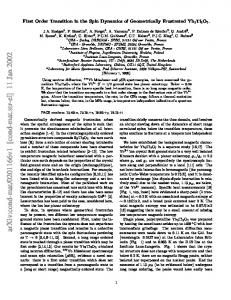
where Si are two component classical vectors of unit length. The sum runs over all nearest neighbor pairs, that is the spin Si has six nearest neighbor spins in the same XY –plane and two in Z–direction in adjacent planes. The ground state is characterized by a planar spin configuration with three spins on each triangle forming a 120◦ structure with either positive or negative chirality (see Fig. 1). The ground state degeneracy is thus twofold like the Ising symmetry, in addition to the continuous degeneracy due to global rotations. In the RG theory one uses the concept of local rigidity which means that the sum of three spins S1 , S2 , S3 on the corners of a triangle is set to zero S1 + S2 + S3 = 0 .

(2)

In this theory the local fluctuations violating this constraint become modes with a gap. Thus they do not contribute to the critical behavior and can be neglected [13]. The constraint in (2) used for an ordinary collinear antiferromagnet with two spins instead of three eliminates also one degree of freedom so that only one is left which means that the critical behavior of antiferromagnet is the same as that of a ferromagnet. In our case we are left with two degrees of freedom. We choose one spin direction and then have one more choice for the chirality, that is the direction of the second spin could be chosen clockwise or counter–clockwise with respect to the first spin. In order to impose local rigidity for the MC simulation, we first partition the lattice into interacting triangles which do not have common corners. This can be done as follows. In each XY –plane one selects in a row one ”supertriangle”. Then one finds two nearest supertriangles which do not share a common corner in the row (they are separated by two head-up and three head-down triangles). This process is repeated. Then one takes the next row until all rows in the XY –planes are filled with triangles which do not share corners, see Fig. 1. All spins are then located on the supertriangles and each spin belongs to only one supertriangle. Local rigidity means that the three spins in each supertriangle form a 120◦ structure. Only in the ground state all the supertriangle have the same orientation. At finite temperature local rigidity means that there are no local fluctuations within a supertriangle, but fluctuations between supertriangles are allowed. The MC updating procedure for the state of the supertriangles is made as follows. At a supertriangle, we take a new random orientation for one of its three spins; next we choose a second spin so as to form a ±120◦ angle with the first spin. For the orientation of the third no freedom is left. The interaction energy between the spins of this supertriangle with the spin of the neighboring supertriangles is calculated in the usual way and we follow the standard Metropolis algorithm to update one supertriangle after the other. We consider L ∗ L ∗ Lz systems , where L ∗ L is the size of the planes, and Lz = 2L/3 the number of planes. L must be a multiple of three so that no frustration occurs because 3

of periodic boundary conditions in the XY –planes. Simulations have been done for systems sizes with L = 12, 18, 24, 30, 36. The order parameter M used in the calculation is M=

3 1 X | Ms | , N s=1

(3)

where Ms (s = 1, 2, 3) is the s-th sublattice magnetization and N = L2 Lz is the total number of the lattice sites. This definition corresponds to the one for the ordinary antiferromagnet with only two sublattices. Instead of alternating signs for the collinear case the non collinear staggered magnetization is obtained by making a rotation of +1200 (−1200 ) for the second (third) magnetization before summing over the three sublattice magnetizations. The chirality κ is defined in the usual way i 2 h κi = √ S1i × S2i + S2i × S3i + S3i × S1i , 3 3 1 X κ= ′| κi | , N i

(4) (5)

where the summation is over all supertriangles and N ′ = N/3 is their number. The chirality κi of one triangle is parallel to the Z-axis and equal to ±1. B. The Stiefel model

The Stiefel model can be derived from the STAR model [13]. We give the main points. In each elementary cell an orthonormal basis ea (i); a = 1, 2

(6)

is defined, where i is the superlattice index. Each spin located in the cell can be represented in this basis Si =

X

sa (i) ea (i) .

(7)

a

If we put this expression into the Hamiltonian (1) we obtain a new Hamiltonian with interactions between the orthogonal vectors ea (x): H=J

Xh ij

e1 (i) · e1 (j) + e2 (i) · e2 (j)

i

.

(8)

The interaction can be chosen negative (or ferromagnetic) and the sum ij is for simplicity over nearest neighbor pairs of a simple cubic lattice instead of a hexagonal lattice since the new spins ea (see Fig. 2 and 3) are no longer frustrated. The chirality κ for the Stiefel model is defined as P

κ =

1 P | i e1 (i) × e2 (i) | . N 4

(9)

The Hamiltonian (8) is similar to the one of the Ashkin-Teller model [14]. Indeed we can give this Hamiltonian a form which is close to it. The interaction energy of two nearest neighbors (ij) with opposite chirality (9) is zero and with the same chirality it is 2 e1 (i)e1 (j) (see Fig. 3). Therefore the Hamiltonian can be written as H=J

X

(1 + σi σj ) Si Sj

(10)

i,j

where σ = ±1 is an Ising spin representing the chirality and Si is an XY –spin. In Hamiltonian of Ashkin and Teller only Ising spins appear. Despite the fact that the Stiefel model is extensively studied, especially in two dimensions, no clear picture emerged. The problem is to know whether there are two transitions, an Ising and a Kosterlitz–Thouless transition, or only one transition of a new type [15,23]. In three dimensions it has been shown that there is only one transition [2,3,5,4]. Here the problem is to determine the order of the transition. The procedure of MC procedure is as follows. At each site one takes a new random orientation for the first vector and chooses for the second vector a perpendicular direction (we have two choices: ±900 , the Ising degrees of freedom). We have two degrees of freedom the same number as for the STAR model. The interaction energy between this dihedral and its neighbors is calculated. If it is lower than the energy of the old state, the new state is accepted. Otherwise, it is accepted only with a probability according to the standard Metropolis algorithm. It is possible to use a cluster MC algorithm [12], but in the case of a strong first order transition there is no reduction of the critical slowing down [17]. Periodic boundary conditions are used. Systems with L = 12, 15, 18, 21, 24 have been simulated. To compare with the size L √ of the STA or the STAR model, we must multiply L by 3. One supertriangle or triangle contains three spins and is represented by one site in the Stiefel model. So we obtain equivalent sizes from 20 to 40. The order parameter M for this model is M=

2 1 X | Ms | , 2N s=1

(11)

where Ms (s = 1, 2) is the magnetization for the vectors eα over all sites and N = L3 is the total number of sites. C. Definitions, histogram methods and finite-size scaling

We use in this work the histogram MC technique developed by Ferrenberg and Swendsen [18,19]. The histogram for the energy PT (E) is very useful for identifing a first order transition. Also the data obtained by simulation at T0 can be used to obtain thermodynamic quantities at temperature T close to T0 . Since the energy spectrum of a Heisenberg spin system is continuous, the data list obtained from a simulation is basically a histogram with one entry per energy value. In order to use the histogram method efficiently, we divided the energy range E < 0 by 10 000 bins. We have verified that we obtain the same results, with our precision, for 30 000 bins. 5

The critical slowing down in a first order transition is greater than in a second order transition because of energy barriers, and thus the time of the simulation, to go from one state to another grows exponentially with the size of the lattice. For this reason we restricted our simulations to systems not too large to have good enough statistics. In each simulation, at least 2 millions (3 millions for the greater sizes) measurements were made after enough Metropolis updating (500 000) were carried out to reach equilibration. For each temperature T we calculate the following quantities (< E 2 > − < E >2 ) C= , NkB T 2 N(< M 2 > − < M >2 ) χ= , kB T N(< κ2 > − < κ >2 ) , χκ = kB T < E4 > , V =1− 3 < E 2 >2

(12) (13) (14) (15)

where M is the order parameter, C the specific heat per site, χ the magnetic susceptibility per site, V the fourth order energy cumulant, < ... > means the thermal average. The finite size scaling (FSS) for a first order transition has been extensively studied [20–22]. A first order transition should be identified by the following properties: a) PT (E) has a double peak. b) The maximum of the specific heat C and the susceptibilities χ and χκ are proportional to the volume Ld . c) The minimum of the fourth order energy cumulant V varies as: V = V ∗ + b L−d ,

(16)

where V ∗ is different from 2/3. d) The temperatures T (L) at which the quantities C, χ or χκ have a maximum should vary as: T (L) = Tc + a L−d .

(17)

All this conditions will be verified for our systems. III. RESULTS

In Fig. 4 the specific heat C of the STAR model is plotted as function of the temperature for various sizes (we note that the maximum is 30 times as large as the usual value of STA which is a sign of a first order transition). The value of the maximum as function of the volume is shown in Fig. 5 for C, χ and χκ . We note that the maxima vary like the volume except for the smaller sizes where further corrections are important. 6

In Fig. 6 the same quantities are shown for the Stiefel model. In all cases the maxima vary for the greater sizes proportional to the volume as they should for a first order transition. In Fig. 7 and 8 we have plotted V as function of T for different sizes L for the STAR and the Stiefel model respectively. We can see that V does not tend to 2/3 (for a second order transition) but to a value V ∗ < 2/3. This value is calculated by fiting the minimum with (16). As result we yield for the STAR model V ∗ = 0.652(2)

(18)

V ∗ = 0.625(3) .

(19)

and for the Stiefel model

The Fig. 9 and 10 show the energy distribution for different sizes at different temperatures for the STAR and Stiefel model. The double peaks observed, even for a very small L, indicate a strong first order transition. With increasing sizes, these two peaks are separated by a region of zero probability, indicating a discontinuity of the energy at the transition. We estimate the correlation length ξ0 by 1/3 of the first size where the two peaks are well separated by a region of zero probability. This is our estimate of the distance needed for two phases to coexist. This method yields the correct answer in the case of Potts models. We obtain ξ0 ∼ 12 for the STAR model and ξ0 ∼ 9 for the Stiefel model (see Fig. 9 and 10). To obtain the critical temperature we can use (17). The results are Tc = 2.2990(5)

(20)

Tc = 2.4428(4)

(21)

for the STAR model and

and for the Stiefel model. We have sizable corrections for the small systems. Comparing the last results with those of Kunz and Zumbach [12] for the case V2,2 similar to ours we agree with their result Tc =2.445. Our results show clearly the first order transition for the STAR and Stiefel model. So we confirm the indication given in [12] for the Stiefel model where in high temperature region ν was determined not too far away from 1/3 which is the value for a first order transition. IV. DISCUSSION

We have shown that the STAR and the Stiefel model have first order transitions. These models are equivalent to the STA in the RG theory, because the constraint of local rigidity is not relevant in the transition region. Consequently the phase transition for the original triangular antiferromagnet STA must also be of first order, and this result holds generally for all systems with a breakdown of symmetry of type O(2) ⊗ Z2 . How can we reconcile our results with those of the MC of the STA model and the experimental results? For the MC simulation of the original frustrated spin system the second order transition is an effect of the finite system size according to Zumbach’s analysis of ”almost second order phase transitions” [25]. The main point of this analysis is that the stable fixed point Fc , 7

known to exist only for the number of components N > Nc , moves into the unphysical complex plane when N < Nc . In our case N = 2, the estimation for Nc is Nc = 3.91 [8] and second order could never occur. Nevertheless this complex fixed point has a large basin of attraction and mimics a behavior of a real fixed point. Only if the system is very large, i.e. if L ≥ ξ0 , where ξ0 is the largest correlation length, the transition will appear of first order. The phenomenon of a crossover between a second order to a first order transition is not so uncommon. An extreme case is the Potts model in two dimensions with q = 5 components, where the transition is known to be of first order [27]. The MC gives always a second order transition with critical exponents of an instable fixed point [28] due to the enormous correlation length ξ0 . If the Hamiltonian is a sum of two terms, one interaction is of the Heisenberg symmetry and the other favors Ising symmetry: H = HHeisenberg + HIsing and if HIsing ≪ HHeisenberg , one has a crossover between a region of Heisenberg type to Ising behavior close to Tc . If the system size is too small we will only see the region controlled by the Heisenberg fixed point and therefore obtain the exponents of the Heisenberg magnet. In a sense we have the same situation if we replace the Heisenberg fixed point by the Zumbach fixed point. However, there is an essential difference: for the fixed point in the complex plane, one has to modify the scaling relation γ/ν = 2 − η + c

(22)

by a constant c different from zero [25]. If the fixed point is real c must be zero. We can use this relation as a criterion for real or complex fixed points. In three dimensions η is usually small, that is ∼ 0.03 (see table VI), but it must be positive [29] and therefore γ/ν ≤ 2 for a genuine second order phase transition. If the ratio γ/ν > 2 the fixed point must be complex. The correction c in the scaling law (22) will depend on the distance of the fixed point from real space. Therefore one expects that c will be greater for the XY (N = 2) case than for the Heisenberg (N = 3) case. For frustrated Heisenberg systems it will be difficult to find out whether ηef f = η − c is negative. With the relation γ/ν = 2−η we obtain η = −0.06 using the results of MC simulation [4] and η = −0.16 from experimental values of Ho [52]. Thus the fixed point is in the complex plan and the second order transition observed in the XY systems has only an “almost second order” character. The effect of imposing local rigidity obviously forces the system to stay away from the region of influence of the complex fixed point Fc and thus permits to ”see” the true first order behavior. Introducing larger coupling constants for inter–plane interactions than for intra–plane interactions [10] seems to have a similar effect as the local rigidity constraint. A further remark concerning MC simulations and the fixed point Fc in the complex plane; Zumbach [25] has shown that the finite size scaling in this case does not hold. The FSS ansatz for the free energy should be replaced by f = L−d g[L/ξ, c2ln(L)] ,

(23)

where g is a function of L/ξ, but also of lnL. The constant c2 is proportional to the constant c of (22). This constant is small and therefore the correction to FSS. Indeed if we take for the true value of η the value of the ferromagnetic case η ∼ 0.03 (see table VI) the value of 8

c will be at most equal to c ∼ 0.03 + 0.06 ∼ 0.1 (see discussion above) and if we compare with 2 − η in (22) this gives an error of 5 %. However, small but not negligible corrections to the standard FSS could explain the differences in MC simulations obtained with different methods (see table V) and also some of the differences in the experimental values (tables I-IV). We will discuss now the experiments in the light of the concepts used. In order to see the first order region the temperature resolution is the limiting factor not the finite size. −1/ν However, they are linked through t0 ∝ ξ0 with ν ∼ 0.5 found by MC and ξ0 depending on the materials studied. The temperature distance t0 = (T − Tc )/Tc could be too small to be measurable. The experiments on CsMnBr3 [31–41], RbMnBr3 [42,43] and CsVBr3 [44] (I) give exponents compatible with those of MC on STA and a second order transition (see table I and V). We can interpret this result by the fact that the systems are under the influence of a complex fixed point and t0 is too small to observe a first order transition. The case CsCuCl3 [47] (table I) is different since the authors observe a crossover from a second order region with exponents compatible with MC on STA for 10−3 < t < 5.10−2 to a region of first order transition for 5.10−5 < t < 5.10−3. For t < t0 ≈ 10−3 one seems to observe the true first order region. Helimagnetic rare earth metals are more complicated as already discussed in the introduction (see also tables II-IV). The results compatible with those of the MC on STA for Ho [51–53] (table II), Dy [53,59,60] (table III) and Tb [64–68] (table IV) can be interpreted as before: the systems are under the influence of Fc . The first order transition for Ho [50] and Dy [57,58] is due to the fact that the measurements were done in the first order region near the critical temperature. The values of the exponent β ∼ 0.39 in the case of Ho and Dy (see table II-III) are not compatible with those found by MC (β ∼ 0.25). This fact can be explained by the presence of a second length scale in the critical fluctuations near Tc related to random strain fields which are localized at or near the sample surface [52]. Thus the critical exponent β measured is of this second length. However the result of β for Tb (table IV) shows values compatible with MC but it has been proved that this second length is present also in Tb [67]. Further measurements to determine β should help in the interpretation. We have tried to give a general picture of the phase transition of frustrated XY spins where the breakdown of symmetry is of type O(2)⊗Z2. We have shown that this transition is first order but usually not seen because of the presence of a fixed point in the complex plane. One way to observe that the behavior is really driven by such a fixed point is the existence of a negative value for η in the Monte Carlo simulations and experimental systems. The method used here is to impose local rigidity. This constraint does not change the behavior of the system but permits the system to stay outside the region of influence of the complex fixed point. So we can rely on the renormalization group study and the true behavior is first order. There is no ”new chiral universality class” in strict sense for our system (N = 2). Another possibility discussed in the literature is that the transition is influenced by the presence of topological defaults which are not visible in the continuum formulation of the RG (for the presence of topological defaults in Stiefel model see [12]). From our experience with the frustrated XY –model we conclude that the true first order transition for the frustrated Heisenberg model cannot be reached in MC simulations. The 9

experimental situation should be similar. However, due to presence of the anisotropies we never reach the Heisenberg first order region but will have a crossover to the Ising or XY region [23]. V. ACKNOWLEDGMENTS

This work was supported by the Alexander von Humboldt Foundation. One of the authors (D.L.) is grateful to Professors B. Delamotte, H.T. Diep and A. Dobry for discussions, and for A.I. Sokolov for the reference to the proof of η ≥ 0.

10

REFERENCES 1

2 3

4 5 6 7 8 9 10 11 12 13

14 15

16 17 18 19 20 21 22 23 24 25

26 27

28 29

30 31

32

Magnetic Systems with Competing Interactions (Frustrated Spin Systems), edited by H.T. Diep (World Scientific, Singapore, 1994). H. Kawamura, Phys. Rev. B 38, 4916(1988), 42, 2610 (1990). H. Kawamura, J. Phys. Soc. Jpn 61, 1299 (1992), 58, 584 (1989), 56,474 (1987), 55, 2095 (1986). M.L. Plumer and A. Mailhot, Phys. Rev. B 50, 16113 (1994). E. H. Boubcheur, D. Loison, and H.T. Diep, Phys. Rev. B 54, 4165 (1996). D. Bailin, A. Love, and M.A. Moore, J. Phys. C 10, 1159 (1977). T. Garel and P. Pfeuty, J. Phys. C L9, L245 (1976). S.A. Antonenko and A.I. Sokolov, Phys. Rev. B 49 15901(1994). S.A. Antonenko, A.I. Sokolov and V.B. Varnoshev, Phys. Lett. A 208, 161 (1995). M.L. Plumer and A. Mailhot, J. Phys.: Cond. Matter. 9i, L165 (1997). H. Kawamura, Prog. Theo. Phys. Supp. 101, 545 (1990). H. Kunz and G. Zumbach,J. Phys. A 26, 3121 (1993). P. Azaria and B. Delamotte, in [1] edited by H.T. Diep (World Scientific, Singapore, 1994), P. Azaria, B. Delamotte,F. Delduc and T. Jolicoeur, Nucl. Phys. B 408, 485 (1993), P. Azaria, B. Delamotte and T. Jolicoeur, Phys. Rev. Lett. 64, 3175 (1990), J. App. Phys. 69, 6170 (1991). J. Askin and E. Teller, Phys. Rev. 64, 178 (1943) E. Granato, J.M. Kosterlitz, J. Lee and M. P. Nightingale, Phys. Rev. Lett. 66, 1090 (1991), J. Lee E. Granato and J.M. Kosterlitz, Phys. Rev. B 44, 4819 (1991), M. P. Nightingale, E. Granato and J. M. Kosterlitz, Phys. Rev. B 52, 7402 (1995), E. Granato and M.P. Nightingale, Physica B 222, 266 (1996). D. Loison and P. Simon, in preparation. W. Janke, Phys. Rev. B 47, 14757 (1993) A. M. Ferrenberg and R. H. Swendsen, Phys. Rev. Let. 61, 2635 (1988). A. M. Ferrenberg and R. H. Swendsen, Phys. Rev. Let. 63, 1195 (1989). V. Privman and M.E. Fisher, J. Stat. Phys. 33, 385 (1983). K. Binder, Rep. Prog. Phys. 50, 783 (1987) A. Billoire, R Lacaze and A. Morel, Nucl. Phys. B 370 773 (1992). D. Loison in preparation. K. Binder, Z. Phys. B 43, 119 (1981). G. Zumbach, Phys. Rev. Lett. 71, 2421 (1993) 2421 (1993), Nucl. Phys. B 413,771 (1994). S.A. Antonenko, A.I. Sokolov, Phys. Rev. E 51, 1894 (1995). R.J. Baxter, Exactly solved models in statistical mechanics. London, Academic Press, 1982. P. Peczak and D.P. Landau, Phys. Rev. B 39, 11 932 (1989). A.Z. Patashinskii and V.I. Pokrovskii, Fluctuation Theory of Phase Transitions, Pergamon press 1979, chap. VII, 6 , The S-matrix method and unitary relations. D. Loison and K.D. Schotte, in preparation. T.E. Mason, Y.S. Yang, M.F. Collins, B.D. Gaulin, K.N. Clausen and A. Harrison, J. Magn. and Magn. Mater 104-107, 197 (1992). T.E. Mason, M.F. Collins and B.D. Gaulin, J. Phys. C 20, L945 (1987). 11

33

34

35 36 37 38

39 40

41 42

43

44 45 46

47

48

49

50 51 53 52

54 55 56

57

58 59 60 61

Y. Ajiro, T. Nakashima, Y. Unno, H. Kadowaki, M. Mekata and N. Achiwa, J. Phys. Soc. Japan 57, 2648 (1988). B.D. Gaulin, T.E. Mason, M.F. Collins and J.F. Larese, Phys. Rev. Lett. 62, 1380 (1989). T.E. Mason, B.D. Gaulin and M.F. Collins, Phys. Rev. B 39, 586 (1989). H. Kadowaki, S.M. Shapiro, T. Inami and Y. Ajiro, J. Phys. Soc. Japan 57, 2640 (1988). J. Wang, D.P. Belanger and B.D. Gaulin, Phys. Rev. Lett. 66, 3195 (1991). H. Weber, D. Beckmann, J. Wosnitza, H.v. L¨ohneysen and D. Visser, Inter. J. Modern Phys. B 9, 1387 (1995). T. Goto, T. Inami and Y. Ajiro, J. Phys. Soc. Japan 59, 2328 (1990). R. Deutschmann, H.v. L¨ohneysen, J. Wosnitza, R.K. Kremer and D. Visser, Euro. Phys. Lett, 17, 637 (1992). M.F. Collins, O.A. Petrenko, Can. J. Phys. 75, 605 (1997) T. Kato, T. Asano, Y. Ajiro, S. Kawano, T. Ihii and K. Iio Physica B 213-214, 182 (1995). T. Kato, K. Iio, T. Hoshimo, T. Mitsui and H. Tanaka, J. Phys. Soc. Japan 61, 275 (1992). H. Tanaka, H. Nakamo and S. Matsumo, J. Phys. Soc. Japan 63, 3169 (1994). H. Hirakawa, H. Yoshizawa and K. Ubukoshi J. Phys. Soc. Japan 51, 1119 (1982). K. Adachi, N. Achiwa and M. Mekata J. Phys. Soc. Japan 49, 545 (1980), U. Schotte, N. St¨ usser, K.D. Schotte, H. Weinfurter, H.M. Mayer and M. Winkelmann, J. Phys.: Condens. Matter 46, 10105 (1994) H. B. Weber, T. Werner, J. Wosnitza H.v. L¨ohneysen and U. Schotte, Phys. Rev. B 54, 15924 (1996). W.C. Koehler, J. App. Phys. 36, 1078 (1965), W.C. Koehler, J.W. Cable, M.K. Wilkinson, and E.O. Wollan, Phys. Rev. 151, 414 (1996). D.A. Tindall, C.P. Adams, M.O. Steinitz and T.M. Holden, J. Appl. Phys. 75, 6318 (1994). D.A. Tindall, M.O. Steinitz and M.L. Plumer, J. Phys. F 7, L263 (1977). K.D. Jayasuriya, S.J. Campbell and A.M. Stewart, J. Phys. F 15, 225 (1985). B.D. Gaulin, M. Hagen and H.R. Child, J. Physique Coll. 49 C8, 327 (1988). T.R. Thurston, G. Helgesen, D. Gibbs, J.P. Hill, B.D. Gaulin and G. Shirane, Phys. Rev. Lett. 70, 3151 (1993) , T.R. Thurston, G. Helgesen,J.P. Hill, D. Gibbs, B.D. Gaulin and P.J. Simpson, Phys. Rev. B 49, 15730 (1994). P. Du Plessis, A.M. Venter and G.H.F. Brits J. Phys. (Cond. Mat.) 7, 9863 (1995). J. Ecker and G. Shirane, Solid State Commun. 19, 911 (1976). G. Helgesen, J.P. Hill, T.R. Thurston, D. Gibbs, J. Kwo and M. Hong, Phys. Rev. B 50, 2990 (1994). S.W. Zochowski, D.A. Tindall, M. Kahrizi, J. Genosser and M.O. Steinitz, J. Magn. Magn. Mater. 54-57, 707 (1986). H.U. ˚ Astr¨om and G. Benediktson, J. Phys. F 18, 2113 (1988). F.L. Lederman and M.B. Salomon, Solid State Commun. 15, 1373 (1974). K.D. Jayasuriya, S.J. Campbell and A.M. Stewart, Phys. Rev B 31, 6032 (1985). P. Du Plessis, C.F. Van Doorn and D.C. Van Delden, J. Magn. Magn. Mater. 40, 91 (1983). 12

62 63 64

65 66

67

68

G.H.F. Brits and P. Du Plessis, J. Phys. F 18, 2659 (1988). E. Loh, C.L. Chien and J.C. Walker, Phys. Lett. 49A, 357 (1974). K.D. Jayasuriya, A.M. Stewart, S.J. Campbell and E.S.R. Gopal, J. Phys. F 14, 1725 (1984). O.W. Dietrich and J. Als-Nielsen, Phys. Rev. 162, 315 (1967). C.C. Tang, P.W. Haycock, W.G. Stirling, C.C. Wilson, D. Keen, and D. Fort, Physica B 205, 105 (1995). K.H. Hirota, G. Shirane, P.M. Gehring and C.F. Majkrzak, Phys. Rev B 49, 11 967 (1994), P.M. Gehring, K.H. Hirota,C.F. Majkrzak and G. Shirane, Phys. Rev L 71, 1087 (1993). C.C. Tang, W.G. Stirling, D.L. Jones, A.J. Rolloson, A.H. Thomas and D. Fort, J. Magn. Magn. Mater. 103, 86 (1992).

13

TABLES Crystal CsMnBr3 CsMnBr3 CsMnBr3 CsMnBr3 CsMnBr3 CsMnBr3 CsMnBr3 RbMnBr3 RbMnBr3 CsCuCl3 CsCuCl3 CsCuCl3

method Neutron Neutron Neutron Neutron Neutron Calorimetry Calorimetry Neutron Calorimetry Neutron Calorimetry Calorimetry

ref. [32] [33] [34] [35] [36] [37] [40] [42] [43] [46] [47] [47]

α

β 0.22(2) 0.25(1) 0.24(2) 0.21(2)

γ

ν

1.01(8) 1.10(5)

0.54(3) 0.57(3)

0.39(9) 0.40(5) 0.28(2) 0.22-0.42 0.25(2) 0.35(5) if 10−3 < t < 5.10−2 > 0.6 if 5.10−5 < t < 5.10−3

TABLE I. Experimental values of critical exponents for compound AXB3

Crystal Thermal expansion Calorimetry Calorimetry Neutron Neutron Neutron Neutron X-ray X-ray

ref. [50] [51] [37] [53] [52] [54] [55] [52] [56]

α order 0.27(2) 0.10-0.22

β

γ

ν

1.14(10) 1.24(15)

0.57(4) 0.54(4)

1st

0.3(1) 0.39(2) 0.39(4) 0.37(1) 0.39(4)

TABLE II. Experimental values of critical exponents for Holmium

14

method Thermal expansion Calorimetry Calorimetry Calorimetry Neutron Neutron Neutron Neutron M¨ossbauer

ref. [57] [58] [59] [60] [53] [54] [61] [62] [63]

α 1st order 1st order 0.18(8) 0.24(2)

β

γ

ν

1.05(7)

0.57(5)

0.38(2) 0.38(3) 0.39(1) 0.335(10)

TABLE III. Experimental values of critical exponents for dysprosium

method Calorimetry Neutron Neutron Neutron X-ray

ref. [64] [65] [66] [67] [68]

α 0.20(3)

β

γ

ν

0.25(1) 0.23(4) 0.53 0.21(2)

TABLE IV. Experimental values of critical exponents for Terbium

ref. [3] [4] [5]

α 0.34(6) 0.46(10) 0.43(10)

β 0.253(10) 0.24(2)

γ 1.13(5) 1.03(4)

ν 0.54(2) 0.50(1) 0.48(2)

η1 -0.09(8) -0.06(4)

βκ 0.45(2) 0.38(2)

γκ 0.77(5) 0.90(9)

νκ 0.55(2) 0.55(1)

TABLE V. Critical exponents by Monte Carlo for O(2) ⊗ Z2 . 1 calculated by γ/ν = 2 − η. The first result [3] comes from a study at high and low temperature and uses of FSS. The second [4] uses the Binder parameter [24] to find Tc and uses the FSS, the third [5] uses the maxima in FSS region. The results βκ , γκ , νκ are the exponents for the chirality.

15

symmetry Z2 O(2) O(3) O(4) O(5) O(6)

α 0.107 -0.010 -0.117 -0.213 -0.297 -0.370

β 0.327 0.348 0.366 0.382 0.396 0.407

γ 1.239 1.315 1.386 1.449 1.506 1.556

ν 0.631 0.670 0.706 0.738 0.766 0.790

TABLE VI. Critical exponents for the ferromagnetic systems calculated by RG [26].

16

η 0.038 0.039 0.038 0.036 0.034 0.031

FIGURES

e (i) 2

e (j)

J

2

e1 (i) -

+

+ -

+ -

+

+ -

+ -

+

+ -

+ -

+

+ -

+ -

+

e1 (j)

a) J

+

+

e2 (i)

FIG. 1. Ground state configuration for the STA and the STAR model. The chirality of each triangle is indicated by + or −. The other ground state configuration with opposite chirality is obtained by reversing all spins. The supertriangles are dark.

e1 (j) e1 (i)

θ

e2 (j)

b)

FIG. 3. a. Dihedral and their interaction. e1 (i) interacts only with e1 (j) not with e2 (j) which interacts with e2 (i). b. Two dihedral with opposite chirality. The energy of the interaction is equal to cos(π − θ) + cos(θ) = 0.

FIG. 2. The dihedral are drawn at the center of each elementary supertriangle.

17

500

C 100

C

400

L=36

χκ

300

50

200

L=30

100

L=24 L=18 0 2.29

2.30

χ

2.31

L=12 2.32

T

2.33

0 0e+00

5e+03

1e+04

V

2e+04

FIG. 6. Maxima of the specific heat C, the FIG. 4. Specific heat for the STAR model susceptibility χ (magnetization) and χκ (chiralfor various sizes as function of temperature. ity) in function of the volume V = L3 for the Stiefel model.

800 χ

0.670

V

600 χκ

0.665

L=36

400

L=30

0.660

L=24

200 C

0.655

0 0e+00

1e+04

2e+04

3e+04

L=18 *

V =0.652(2)

4e+04

V

0.650 2.29

2.30

2.31

2.32

T

FIG. 5. Maxima of the specific heat C, the susceptibility χ (magnetization) and χκ (chiralFIG. 7. V as function of temperature for ity) in function of the volume V = L2 · Lz for different sizes for the STAR model. The . . . line the STAR model. indicate the value of V ∗ = 2/3 for the second order transition. The broken line is our estimate of V ∗ at the critical temperature Tc = 2.2990.

18

FIG. 9. Energy histogram P (E) as function of energy per site E for the STAR model for various sizes L at different temperatures of simulation: T12 = 2.3136, T18 = 2.3065, T24 = 2.3020, T30 = 2.30085, T36 = 2.29968.

0.67

V 0.66

L=24

0.65

L=21 L=18 L=15

0.64

0.63

L=12 *

V =0.625(3)

0.62 2.439

2.449

T

2.459

0.002

P(E)

FIG. 8. V as function of the temperature for different sizes for the Stiefel model. The . . . line indicate the value of V ∗ = 2/3 for the second order transition. The broken line is our estimate of V ∗ at the critical temperature Tc = 2.4428.

L=24

0.002

L=21

0.001

L=18 L=15 L=12

0.001

0.000

P(E) L=36 L=30

0.002

L=24 L=18

0.001 L=12

0.000 −2.0

−4

−3

−2

E

FIG. 10. Energy histogram P (E) as function of energy per site E for the Stiefel model for various sizes L at different temperatures of simulation: T12 = 2.4495, T15 = 2.4468, T18 = 2.44525, T21 = 2.44425, T24 = 2.44377.

0.004

0.003

−5

−1.5

−1.0

E

19