Incomplete Pattern Classification using a Multi

Incomplete Pattern Classification using a Multi-Task Approach ´ ´ Pedro J. GARCIA-LAENCINA, Jos´e-Luis SANCHO-GOMEZ Dpto. Tecnolog´ıas de la Informaci´on y las Comunicaciones, Universidad Polit´ecnica de Cartagena Cartagena-Murcia, 30202, Spain. E-mail: [email protected] An´ıbal R. FIGUEIRAS-VIDAL ˜ y Comunicaciones, Universidad Carlos III de Madrid Dpto. Teor´ıa de Senal Legan´es-Madrid, 28911, Spain.

ABSTRACT Missing data present a challenge to many pattern classification tasks. One of the most recommended ways for dealing with unknown values is missing data imputation. This paper presents an useful neural network approach that combines the classification and the missing data imputation using Multi-Task Learning. An effective cost function is also proposed that tends to provide imputed values for the missing ones that enable to get a better classification accuracy preserving the input data distribution. Its performance is tested using both artificial and real datasets. Keywords: Pattern Classification, Missing Data, Multi-Layer Perceptron, Multi-Task Learning, MAP estimation. 1. INTRODUCTION In many applications of pattern classification [1], [2], a part (sometimes considerable) of the data values is missing. This common drawback is known as Missing Data (incomplete feature vector) [3], [4]. Data may contain unknown features due to different reasons, e.g., data collection procedure can be imperfect, sensor failures producing a distorted or unmeasurable value, data occlusion by noise, non-response in surveys [3]. A recommended approach for dealing with unknown values is missing data imputation, i.e., to estimate and to fill in missing values using all the available information. Following this approach, missing features are estimated from the available data, and after imputation is done, a classifier is trained using the edited training set (i.e., complete patterns and incomplete vectors with imputed values). Up to now, most used incomplete pattern classification techniques divide the problem in two separated and isolated tasks, imputation task and classification task, which are solved by different learners. This paper presents a FeedForward Neural Network (FFNN) approach that combines the classification and the missing data imputation in one architecture using Multi-Task Learning (MTL) [5]–[7]. In particular, this paper extends our recent works on MTL networks for incomplete pattern classification [8], [9]. Our approach uses the incomplete features as extra tasks, and learns them in parallel with the main classification task. Outputs that learn incomplete features are used to estimate missing values during learning process. Imputed values are those that contribute to improve the classification accuracy, because the learning of imputation tasks is oriented by the learning of the main task. During Acknowledgments: This work is partially supported by Ministerio de Educaci´on y Ciencia under grant TEC2006-13338/TCM, and by Fundaci´on S´eneca (Consejer´ıa de Educaci´on y Cultura de Murcia) under grant 03122/PI/05.

the training stage, network weights are updated iteratively in order to minimize a cost function. It has two components, an error function for the classification task (cross-entropy error function), and also, an error function for the imputation tasks. This kind of tasks are regression problems, being the quadratic error function one of most used for solving them. It can provide good results, but this error function does not consider the input data distribution. Besides, obtained imputations can be unlikely in some problems, by considering its input data distribution. For solving these drawbacks, a new MAP-based cost function is proposed to estimate missing data. The goal of this work is to find substitution (imputed) values for the missing ones that enable to get a better classification performance preserving the input data distribution. The remainder of this paper is organized as follows. Section 2 shows the used nomenclature for classification with missing data. Next, in Section 3, an MTL network to classify incomplete patterns is described. Section 4 explains its learning and operation modes, emphasizing both the cost functions to be minimized during the training, and the proposed MAP-based cost function. Section 5 shows obtained results. Finally, conclusions and future works end this paper.

2. PATTERN CLASSIFICATION WITH MISSING DATA Let us assume a set of N labeled incomplete patterns† , D = {(x(n) , t(n) , m(n) )}N n=1 , where x(n) is the n-th input vector with d features (x(n) = (n) (d) {xj }dj=1 ), labeled as t(n) , with c possible classes; mj (n) are binary variables taking value 1 if xj is unknown, 0 otherwise. We also define the vector a = [a1 , a2 , ..., am ], whose components indicate the m incomplete attributes in the data set. Thus, for example, if x2 and x4 are the attributes with missing data in the whole data set (i.e., X presents at least one missing value in the attributes x2 and x4 ), then a = [a1 , a2 ] = [2, 4]. This work assumes that the missing data is missing completely at random (MCAR), meaning that the probability that an input (n) (n) feature xj is missing is independent to the value of xj or to the value of any other variables [3]. For classification tasks, it is convenient to use a 1-of-c codification so that if, for example, there are three possible classes (c = 3) and the n-th pattern belongs to the second one, its target vector will be t(n) = (0, 1, 0). † In the following, the terms pattern, observation, input vector, and sample are used as synonyms.

3. MTL APPROACH TO CLASSIFY INCOMPLETE PATTERNS Suppose that a c-class classification problem is described by N input vectors. Each input vector is composed of d features or attributes. Consider that m features are incomplete, with m ≤ d. Following the MTL framework [8], [9], this problem is composed of a main task, a classification task with c classes, and m secondary tasks, imputation tasks associated to each one of the m features with missing values. All tasks are learned in parallel by means of an MTL network with a common hidden layer, which is shown in Figure 1(a). Output layer has c output units to learn the classification task, y(C) , and one ′ output unit for each secondary task, yk(M) ′ , with k = 1, . . . , m. There is an input unit for each feature, and also, c extra input units associated to the classification target. These extra inputs (classification targets) are used as hints to learn the secondary imputation tasks. In the common hidden layer, the number of hidden neurons (Nh ) depends on the problem to be solved. All units are full-connected by weights. We use this notation for (1) weights: wi,j denotes a weight going from input unit i to hidden (1) (2) unit j, w0,j is the bias for hidden unit j; and so, wj,k denotes a weight in the second layer going from hidden neuron j to (2) output unit k, w0,k is the bias for output unit k. In the MTL network, hyperbolic tangent activation functions are used in the hidden layer [8], [9]. Figure 1(b) shows the implemented hidden neuron. Hidden neurons are different to the classical neuron, because they compute different outputs for the distinct tasks to be learned. In particular, they do not include in the sum product

j

w (1 ) i,j

zj,c

) (1 j d,

zj,c+1

w

(1 d+ ) 1, j

xd t1 x1 xd t1

) (1 j ,

xi

zj,1

w1

x1

tc

d+ c,j

o(M) m

w

o(M) 1

o(C) c

w (1 )

o(C) 1

zj,c+m

(b)

Fig. 1. In (a), an MTL network with a common hidden layer that learns the classification and the imputation tasks at the same time is shown. Fig. 1(b) shows the implemented hidden neuron that computes different outputs depending on the output unit where they are addressed. Biases are implicit for simplicity.

the input signal that they have to learn in the corresponding output unit, for avoiding direct connections to map the input as output [5], [8], [9]. The j-th hidden neuron outputs are computed according to the following expressions, For k = 1, ..., c à d ! X (1) (1) zj,k = f wi,j xi + w0,j (1) i=1

For k = c + 1, ..., c + m 



c d X X  (1) (1) (1) zj,k = f  w x + wd+i,j ti + w0,j  i i,j   i=1 i6=ak′

i=1

(C) yk

=

gC

ÃN h X

(2) wj,k zj,k

+

j=1

(M ) yk′

=

gM

ÃN h X

!

,

+

(2) w0,k′ +c

(2) w0,k

(2) wj,k′ +c zj,k′ +c

(3)

j=1

!

,

(4)

where gC (·) is the softmax activation function and gM (·) is the linear activation function. As we have already mentioned, the total target vector is composed of the classification task target vector, tk , and the components corresponding to each feature with missing values (secondary tasks), xak′ . In the next section, the training procedure of this MTL network is explained by considering different cost functions for estimating missing data. 4. TRAINING AND OPERATION STAGES Cost Functions for Main and Extra Tasks During the training stage, the network weights are changed to obtain outputs that are accurate estimations of the desired outputs. In order to measure how accurate is the estimation, a cost function (or error function) is defined for giving a measure of the discrepancy between the predicted values (supplied by the network) and the desired values. The purpose of the learning is to minimize this cost function. In this work, the cost function is defined as m X C = C (C) + C (M) = C (C) + Ck(M) (5) ′ k′ =1

where C is the cost of the main classification task, and Ck(M) ′ is the cost of the secondary imputation task associated to the learning of the incomplete attribute xak′ . Depending on the type of tasks to be learnt, different choices of cost function can be considered. For classification tasks, the goal is modeling the posterior probabilities of class membership, conditioned on the input variables. In these problems, the targets are binary variables (represented with a 1-of -c coding scheme), and it is convenient to minimize the cross entropy cost function [2]. Therefore, in the MTL network, we consider the cross entropy as the classification cost function C (C) , which for two classes (c = 2) is given by, (C)

tc

(a)

where k′ = k − c in Equation 2 (i.e., k′ = 1, . . . , m), and f (·) is the hyperbolic tangent activation function. Finally, the network outputs are obtained by a combination of the outputs of the Nh hidden neurons using a second layer (2) of processing units wj,k ,

(2)

C (C) = −

N n X

n=1

o t(n) ln y (n,C) + (1 − t(n) ) ln(1 − y (n,C) ) , (6)

and for multiple classes (c > 2) is given by, C (C) = −

c N X X

(n)

(n,C)

tk ln yk

.

(7)

n=1 k=1

On the other hand, for imputation tasks, which are regression problems, the basic goal is to model the conditional distribution of the output variable, given the input data. In this work, we have an estimator (each one of the imputation output of the MTL network) for each incomplete attribute xak′ , i.e., for each

E(δ)

(n)

secondary imputation task. The term δk′ denotes the error of the k′ -th missing data estimator for the n-th observation, ³ ´ (n) (n,M) δk = yk − xa(n) (8) k (n,M)

where yk′ is the estimation of the k′ -th incomplete attribute (n) provided by the MTL network when it is fed with x(n) , and xak′ is the desired imputed value. Since E(δ) is the error function to measure the estimation accuracy for each observation, the cost function has the form (M )

Ck ′

=

N X

(n)

E(δk′ )

(9)

n=1

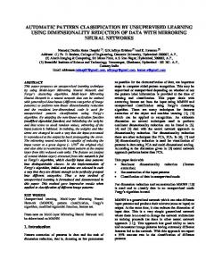
Different choices of E(δ) give different estimators. It is usual to consider the sum-of-squares cost function, where the error function is the quadratic error E(δ) = δ 2 , showed in Figure 2(a). In this case, it is noted that large errors are particularly costly, and so, one of its potential difficulties is that it receives large contributions from outliers. Using a bayesian philosophy [10], this cost function minimization provides a Minimum Mean Square Error (MMSE) estimator, and moreover, the optimal solution of this optimization is the mean of the conditional posterior Probability Density Function (PDF), p(xak′ |x(n) , t(n) )

(10)

Other possible cost function is the “hit-or-miss” error, which is showed in Figure 2(b). It assigns no cost for small error, and a E(δ) = δ 2

E(δ) ___

δ

1

ǫ

−ǫ

(a)

δ

(b)

Fig. 2. Error functions for MMSE and MAP estimation. Quadratic error function is shown in (a); whilst the hit-or-miss error function is shown in (b).

cost of 1 for all errors in excess of a threshold error, i.e., ½ 0 |δ| < ǫ (11) E(δ) = 1 |δ| > ǫ where ǫ is a threshold, which determines the quality of the estimation we want to achieve. When ǫ close to zero, the estimator that minimizes the “hit-or-miss” error is the mode (location of the maximum) of the posterior PDF shown in Eq. (10). It is termed the Maximum A Posteriori (MAP) estimator. From its definitions and from Figure 2, the “hit-or-miss” error is a non smooth function, whist the quadratic error is a differentiable function, which is a necessary condition in a neural network trained by means of gradient information [2]. Besides, the “hitor-miss” function assigns the same cost for different “hits”, without considering how good the estimations are. Based on these observations, we introduce an unified error function given by, E(δ) = 1 − exp(−αδ 2 )

(12)

Figure 3 shows the proposed cost function for different choices of α. For lower values of α, the minimization of Eq. 12 tends to provide an MMSE-based estimator for a large range of δ values,

α > 1 α = 1

__

1

α < 1

δ Fig. 3. Proposed error function. It depends on the parameter α, which determines what kind of estimation (MMSE-based or MAP-based estimation) will be obtained.

whereas for higher values of α, it tends to be an MAP-based estimator. During the learning phase, different values of α are used iteratively; we begin with a lower α and, in each iteration, the MTL network is trained until convergence, and after that, α is increased. In other words, we start with an MMSE-based estimator, and as α is increased, an MAP-based estimator is obtained. This cost function presents desirable and appropriate characteristics to learn secondary imputation tasks, as we show in the next section using a simple classification example with missing data. Unlike the classical quadratic error minimization, the main advantage of the proposed cost function is that the obtained imputed values preserve the input data distribution. All the presented error functions for the secondary tasks (n) depend on the differences δk′ . If x(n) is incomplete, the (n) computation of δk′ for incomplete imputation targets cannot be done because they are unknown, and they cannot contribute to learning process. For this reason, differences associated to every incomplete imputation target is established to zero. After obtaining the differences, the derivatives of Eq. (5) with respect to the weights can be evaluated, and these derivatives are used to find weight values that minimize Eq. (5) by gradient descent method in sequential mode with adaptive learning rate and momentum term. Furthermore, incomplete values are estimated using the imputation outputs during training stage. Learning of the classification task affects to these imputed values, and so, this imputation is oriented to solve the classification task. Imputation is done when the learning of imputation tasks is stopping [8], [9]. After the training is early stopped using the cross validation procedure, the α parameter value is increased, and the training is repeated. Operation Stage Once the network is trained, it is used to classify new input patterns. If x(n) is completely known, the MTL network directly classifies it using the classification output y(n,C) . But if x(n) has (n,M ) unknown values, outputs yk′ associated to the incomplete features (secondary tasks) are used for imputing those values. Nevertheless, these outputs depends on the components of t(n) which are not known. In order to solve that this target class is not available during the operation stage, all possible values of t are checked, and the most consistent value is selected. We define the consistency of a particular value of t as the difference between the target class t and the output y(C) corresponding to the main (classification) task produced by the network. The lower this difference, the larger will be the consistency.

5. EXPERIMENTAL RESULTS

is more complicated with incomplete vectors B and C, but in any case, the MAP-based cost function minimization will obtain more likely imputations than the quadratic error.

2

1.5

A Feature 2

Finally, it must be stressed that the MTL network to classify incomplete patterns is not only a multi-output FFNN, where one output is discrete-valued (classification output) and the other ones are continuous-valued (regression outputs for imputing missing values). The MTL network provides a missing data imputation oriented to solve the classification task, i.e., this method provides imputed values that enable to get a better classification performance. In addition to this, our method combines the classification and the missing data imputation in one FFNN. Experimental results on real and artificial classification data sets are given in the next section to show the usefulness and effectiveness of the MTL approach.

1

B C 0.5

D

In this section, the imputation and classification performances of the MTL network are evaluated. First, a two-dimensional synthetic problem is used to illustrative that the MAP-based cost function provides an accurate estimation of missing values by considering its input data distribution. Secondly, a real incomplete classification problem is used to compare the classification accuraccy provided by the MTL approach and other machine learning procedures.

0

−0.5 −2

−1.5

−1

−0.5

0

0.5

1

1.5

2

Feature 1

(a) 0.8

1 A

0.8

0.6

Two-dimensional synthetic data set

B

0.6 0.4

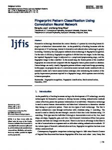
Imputation performance of the MTL approach with the MAPbased cost function is illustrated on a two-dimensional synthetic classification problem composed of five Gaussian components‡ , which is modeled on a dataset used by Ripley [1]. Figure 4(a) shows this synthetic classification problem, where an horizontal line represents the x2 coordinate of an input vector with its first attribute is unknown. Figure 4(b) shows the class conditional posterior PDF of x1 given x2 for each one among the four incomplete patterns labeled in Figure 4(b) as A, B, C and D. As we can see on this figure, missing data estimation and pattern classification can be a hard issue in some cases. Assume that the incomplete vectors A-D are unlabeled. In our approach, an incomplete feature is estimated by means of an MTL network using as inputs the rest of attributes and the target class. Besides, MTL transfer provides that missing data estimation is oriented by the classification learning. As we can see on Figure 4(b), observation A must belong to “circle” class, and its imputed value must be clearly concentrated around x1 = +1, because it provides a high value in the class conditional PDF. In this case, the estimations obtained by the minimization of the quadratic error and proposed error function are identical, because mean and mode are the same. In contrast, it is clear that observation D must also belong to “circle” class, but its imputed value must be near to x1 = −0.7 or x1 = +0.3, which are equally probable. In this case, the MMSE provides an imputation around the mean, i.e., around x1 = −0.2, what is a not accurate estimation because it is an unlikely value; whislt the proposed error minimization, which tends to be a MAP-based estimation, the imputation is located close a maximum of the posterior PDF for the “circle” class. On the other hand, missing data estimation ‡ The mean vectors for each one of the five components are µ = 1 (1, 1)T , µ2 = (−0.7, 0.3)T , µ3 = (0.3, 0.3)T , µ4 = (−0.3, 0.7)T , T µ5 = (0.4, 0.7) ; the covariances are all isotropic: Σj = 0.03I; all five components has the same number of observations, generating 250 samples as training set and 1000 samples as test set.

0.4 0.2

0.2

0 −2

−1

0

1

2

1 0.8

0 −2

0

1

2

−1

0

1

2

1 C

0.8

0.6

0.6

0.4

0.4

0.2

0.2

0 −2

−1

−1

0

1

2

0 −2

D

(b) Fig. 4. Synthetic two-class data. In (a), “circles” and “diamonds” denotes complete patterns from the two classes. Horizontal dashed lines show the x2 coordinate of a pattern with x1 missing. In (b), it is showed the class conditional PDF of x1 given x2 corresponding to the four patterns A-D in (a). A continuous line is used for “circle” class and a dashed line for “diamond” class.

The MTL network performance (using the MAP-based cost function of Equation 12) is evaluated in this synthetic problem inserting 10 % missing data randomly in the first attribute in both training and test set. Figure 5 shows the 2-D synthetic problem, where “circles” and “diamonds” denote the complete patterns, and incomplete patterns are represented by horizontal lines (continuous lines for the “circle” class and dashed lines for the other class). Moreover, the obtained decision frontier by the MTL network is shown for different α values in the proposed function, and also the input vectors with imputed values, which are represented in black color. As we can see on the Figure 5(a), imputed data are around the mean of the conditional PDF. The MTL network provides more likely imputations as the α values are higher, i.e., the imputation output y1(M) tends to provide an MAP estimator of the incomplete feature x1 . Moreover, these imputed values are focused to solve the classification task.

MTL Neural Network (Nh=5) using Proposed Cost Function with α=1/3 4

3

3

2

2

1

1

Feature 2

Feature 2

MTL Neural Network (Nh=5) using Proposed Cost Function with α=1/5 4

0

0

−1

−1

−2

−2

−3

−3

−4 −3

−2

−1

0

1

2

−4 −3

3

−2

−1

Feature 1

(a) α =

1 5

(b) α =

3

3

2

2

1

1

0

−1

−2

−2

−3

−3

−1

0

1

2

−4 −3

3

−2

−1

Feature 1

(c) α =

1 2 4

3

2

2

1

1

Feature 2

Feature 2

0

1

2

3

(d) α = 1.0

3

0

0

−1

−1

−2

−2

−3

−3

−1

1 3

MTL Neural Network (Nh=5) using Proposed Cost Function with α=3.0

4

−2

3

Feature 1

MTL Neural Network (Nh=5) using Proposed Cost Function with α=2

−4 −3

2

0

−1

−2

1

MTL Neural Network (Nh=5) using Proposed Cost Function with α=1.0 4

Feature 2

Feature 2

MTL Neural Network (Nh=5) using Proposed Cost Function with α=1/2 4

−4 −3

0

Feature 1

0

1

2

−4 −3

3

−2

−1

Feature 1

0

1

2

3

Feature 1

(e) α = 2.0

(f) α = 3.0 MTL Neural Network (N =5) using Proposed Cost Function with α=5.0 h

4

3

2

Feature 2

1

0

−1

−2

−3

−4 −3

−2

−1

0

1

2

3

Feature 1

(g) α = 5.0 Fig. 5. Obtained results in the synthetic two-class dataset (10% of missing data in the first attribute) using the MTL network (with Nh = 5 neurons) for different α values in the proposed cost function. Input data have been normalized to zero mean and unity variance.

Pima Indians Data This problem consists of a training set with 300 samples, where 100 samples are incomplete; and a test set of 332 samples [1]. Each input vector has eight attributes. In particular, three attributes are incomplete: x3 , x4 and x5 , with 4.33%, 32.67% and 1.00% as missing data percentages respectively. The document⋆ missclassification test error rate without imputation is around 22.5%. The MTL approach with the MAP-based cost function for the extra tasks (labeled as MAP-MTL) is compared with the MTL network which uses the quadratic error as the cost function to be minimized (labeled as MMSE-MTL). In addition, we also compare with other methods for classifying patterns with missing values, such as the K-Nearest Neighbour (KNN) imputation approach [11]; and also, the Reduced Neural Networks (Reduced NNs) method [12], where a set of FFNNs is created, and each one of them is trained to learn each possible combination of features with unknown values using as inputs the remaining complete features. Table 1 summarizes the obtained results (they are the averages over ten trials). In both procedures, another model (i.e., a FFNN) performs the classification with the imputed set. In all tested methods, the model parameters has been selected by the 10-fold stratified cross validation procedure. As we can see on it, the MTL approaches outperform the other tested procedures. Method KNN Reduced NNs MMSE-MTL MAP-MTL

% Error (mean ± standard deviation) 21.02 ± 0.33 19.76 ± 0.58 19.68 ± 0.18 19.59 ± 0.54

Table 1. Obtained misclassification test error rates for Pima Indians.

6. CONCLUSIONS AND FUTURE WORKS Missing data is a common drawback in a huge number of real-life classification problems. A classical way to deal with unknown values is missing data imputation. This paper describes an useful FFNN approach which combines the classification and the missing data imputation using MTL. In addition to this, an efficient cost function has been proposed for obtaining MAPbased missing data estimators. This cost function depends on the parameter α, which determines what kind of estimation (MMSEbased or MAP-based estimation) will be obtained. Using it, the MTL network provides more likely imputations as the α values are higher. Our approach provides a missing data imputation oriented to solve the classification task preserving the input data distribution. Obtained results on two classification problems show the usefulness of the MTL approach. This paper will stimulate future works in several directions. Some of them are doing an extensive comparison with other solutions for classifying incomplete input data [13]–[15], testing in more decision problems, and using measures of relationship between tasks [6]. 7. REFERENCES [1] B. D. Ripley, Pattern Recognition and Neural Networks. New York, USA: Cambridge University Press, 1996. ⋆ http://www.is.umk.pl/projects/datasets.html Last accessed on December 2007.

[2] C. M. Bishop, Neural Networks for Pattern Recognition. Oxford, UK: Oxford University Press, 1995. [3] R. J. A. Little and D. B. Rubin, Statistical Analysis with Missing Data, 2nd ed. New Jersey, USA: John Wiley & Sons, 2002. [4] J. L. Schafer, Analysis of Incomplete Multivariate Data. Florida, USA: Chapman & Hall, 1997. [5] R. Caruana, “Multitask learning,” Ph.D. dissertation, Carnegie Mellon University, 1997. [6] D. L. Silver, “Selective transfer of neural network task knowledge,” Ph.D. dissertation, University of Western Ontario, 2000. [7] P. J. Garc´ıa-Laencina, A. R. Figueiras-Vidal, J. Serrano-Garc´ıa, and J. L. Sancho-G´omez, “Exploiting multitask learning schemes using private subnetworks.” in International Work-Conference in Artificial Neural Networks (IWANN 2005), ser. Lecture Notes in Computer Science, J. Cabestany, A. Prieto, and F. S. Hern´andez, Eds., vol. 3512. Springer, 2005, pp. 233–240. [8] P. J. Garc´ıa-Laencina, J.-L. Sancho-G´omez, and A. R. FigueirasVidal, “Pattern classification with missing values using multitask learning,” in International Joint Conference on Neural Networks (IJCNN 2006). Vancouver, BC, Canada: IEEE Computer Society, 16-21 July 2006, pp. 3594–3601. [9] P. J. Garc´ıa-Laencina, J. Serrano-Garc´ıa, A. R. Figueiras-Vidal, and J.-L. Sancho-G´omez, “Multi-task neural networks for dealing with missing inputs,” in Bio-Inspired Modeling of Cognotive Tasks (IWINAC 2007), ser. Lecture Notes in Computer Science, J. Mira and J. R. Alvarez, Eds., vol. 4527. Springer, 2007, pp. 282–291. [10] S. M. Kay, Fundamentals of Statistical Signal Processing: Estimation Theory. Prentice Hall, 1993. [11] G. Batista and M. C. Monard, “A study of k-nearest neighbour as an imputation method.” in Hybrid Intelligent Systems, ser. Frontiers in Artificial Intelligence and Applications, A. Abraham, J. R. del Solar, and M. K¨oppen, Eds., vol. 87. IOS Press, 2002, pp. 251–260. [12] P. K. Sharpe and R. J. Solly, “Dealing with missing values in neural network-based diagnostic systems,” Neural Computing and Applications, vol. 3, no. 2, pp. 73–77, 1995. [13] Z. Ghahramani and M. I. Jordan, “Supervised learning from incomplete data via an EM approach,” in Advances in NIPS, J. D. Cowan, G. Tesauro, and J. Alspector, Eds., vol. 6. Morgan Kaufmann Publishers, Inc., 1994, pp. 120–127. [14] T. Marwala and S. Chakraverty, “Fault classification in structures with incomplete measured data using autoassociative neural networks and genetic algorithm,” Current Science, vol. 90, no. 4, pp. 542–548, 2006. [15] K. Jian, H. Chen, and S. Yuan, “Classification for incomplete data using classifier ensembles,” in International Conference on Neural Networks and Brain, M. Zhao and Z. Shi, Eds., Beijing, China, October 2005, pp. 559–563.