rating error recovery in the imprecise computation model. In that model each task ... In a hard real-time system each task must provide a logi- cally correct output ...
Incorporating Error Recovery into the Imprecise Computation Model � Hakan Aydın, Rami Melhem, Daniel Moss´e Department of Computer Science University of Pittsburgh Pittsburgh, PA 15260 (aydin, melhem, mosse)@cs.pitt.edu
Abstract In this paper, we describe optimal algorithms for incorporating error recovery in the imprecise computation model. In that model each task comprises a mandatory and an optional part. The mandatory part must be completed within the task’s deadline even in the presence of faults and a reward function is associated with the execution of each optional part. We address the problem of optimal scheduling in an imprecise computation environment so as to maximize total reward while simultaneously guaranteeing timely completion of recovery operations when faults occur. Furthermore, in order to prevent run-time overhead we enforce that no changes in the optimal schedule should be necessary as long as no error is detected in mandatory parts. Independent imprecise computation tasks as well as tasks with an end-to-end deadline and linear precedence constraints are considered. We present polynomial-time optimal algorithms for models with upper and lower bounds on execution times of the optional parts and for reward functions represented by general nondecreasing linear and concave functions.
1 Introduction and Related Work In a hard real-time system each task must provide a logically correct output before its deadline. The consequences of missing a deadline in a hard real-time environment may be serious, even catastrophic. On the aother hand, an approximate but timely result may be acceptable in many application areas. Examples of such applications are multimedia applications [15], image and speech processing [6, 8, 18], time-dependent planning [5], robot control/navigation systems [20], medical decision making [10], information gathering [9], real-time heuristic search [11] and database query processing [19]. The imprecise computation approach is a technique of improving the responsiveness and resource utilization of systems where requirements are less stringent than hard-real time envi� This work has been supported by the Defense Advanced Research Projects Agency (Contract DABT63-96-C-0044).
ronments [17, 12]. In this model, every real-time task is composed of a mandatory part and an optional part. The mandatory part should be completed by the task’s deadline to yield an output of minimal quality. The optional part may be executed after the mandatory part while still before the deadline, if the application objectives justify doing so. The quality of the final result improves as the optional part runs longer. In the previous studies it is generally assumed that the quality improvement is a linear function of the optional service time; more general and possibly non-linear functions are usually not considered. An alternative model is Increasing-reward-with-increasingservice (IRIS model) [7], where each task can be considered as entirely optional and a task executes for as long as the scheduler allows. However, the more general case of non-linear concave reward functions are addressed in this work. Extensions to models with mandatory parts and dynamic arrivals are described in [7]. The notion of reward in the IRIS model is analogous to that of precision error in the Imprecise Computation model. Linear and general concave functions represent most of the real-world applications such as those mentioned above [6, 8, 18, 15, 5, 20, 11, 9, 19]. Note that the first derivative of a nondecreasing concave function is nonincreasing. In this paper, we focus on linear and concave reward functions. Maximization of the total reward in a system of tasks with 0/1 constraints, where no reward is accrued for a partial execution was shown to be NP-Complete [17]. Continuous convex reward functions results also in an NP-Hard problem [2]. Although the imprecise computation models allow for greater scheduling flexibility, the timely completion of mandatory parts, even in the presence of faults, is still of utmost importance. A first study incorporating error recovery operat ions in the imprecise computation model has appeared in [3]. An extension to on-line scheduling was described in [4]. An important assumption of these works is the a priori knowledge of worst-case fault profile per task. This information is much more difficult to obtain as compared to the maximum number of faults of the entire task set: without information about the fault profile one should provison for simultaneous occurrences of all the faults for all the tasks, which may yield the rejec-
tion of many task sets and the low CPU utilization. Furthermore, even when the task set is accepted, the schedule needs to be updated on-line whenever a mandatory part completes successfully (without failure). As the authors observe in [3], this approach becomes prohibitively expensive in systems with low fault rates, which is usually the case. Also, the reward (error) functions are assumed to be all linear and all tasks independent. In this paper, we consider the more general case of concave reward functions and also examine task sets with linear precedence constraints along with independent tasks. Moreover, our fault model assumes at most k faults within the system and requires that the FT-Optimality of the schedule be preserved as long as no fault occurs. This drastically reduces the run-time overhead when compared with [3], since faults are unusual events in every practical system. The work in this paper is based on the observation that, even when the system is overloaded, the time assigned to optional parts in the imprecise computation model provides opportunities for recovery of tasks, in case an error is detected. We address the problem of optimally assigning service times to tasks in order to simultaneously guarantee error recovery and maximize total reward. Further, our solution has the desirable property that it eliminates any dynamic re-adjustment of the schedule (hence, run-time overhead), as long as no errors are encountered. We present polynomial-time solutions to faulttolerant scheduling problems with upper bounds on service times; our solution works for arbitrary non-decreasing concave reward functions.
2 System Model
2.1 Task Model
We consider a set T composed of n imprecise computation tasks T1 ; T2; : : :; Tn , all ready to run on a uniprocessor system. Each task Ti consists of a mandatory part Mi and an optional part Oi . The length of the mandatory part is denoted by mi ; each task must receive at least mi units of service time in order to provide output of acceptable quality. The optional part Oi becomes ready for execution only when the mandatory part Mi completes. We analyze and provide solutions for two models which differ by the nature of precedence relations. The chain model considers linear precedence constraints among tasks with a common end-to-end deadline D, which is also equal to the period if the task set is periodic. In view of precedence constraints, an optional part Oi must execute after the mandatory part Mi and before Mi+1 . The independent tasks model is identical to the chain model with the only exception that different tasks have no dependence relations. However, a mandatory part Mi must still complete before Oi may start. Associated with each optional part of a task is a reward function Ri(t) which indicates the reward accrued by task Ti when it receives t units of service beyond its mandatory portion. Ri (t) is of the form:
�
if 0 � t � o R (t) = FF (t) (1) (o ) if t > o where F is a nondecreasing, concave and continuously differentiable function over nonnegative real numbers and o is the length of entire optional part O . Note also that in this formulation, by the time the task’s optional execution time t reaches the threshold value o , the reward accrued ceases to i
i
i
i
i
i
i
i
i
i
increase. Given a task set T, a schedule for T determines the amount of service each task receives. A feasible schedule exists if and only if it is possible to complete all the mandatory parts before the deadline; it is clear that Pn this condition is equivalent to P n . If d = D ? mi is the slack available for m � D i i=1 i=1 optional portions, then the foregoing discussion indicates that no feasible schedule exists if d < 0. The Total Reward of an imprecise computation schedule S is REWS
=
P n
=1
R (t ) where t i
i
i
is the amount of service that
optional part Oi receives in S. A feasible schedule is optimal if it maximizes the total reward accrued. i
2.2 Fault Model
We assume that at most k faults may occur during the execution of the task set. However, we develop and present our methodology first in the context of a single fault model (that is k = 1) for the sake of simplicity. The extension of this framework to the multiple faults case is straightforward and presented in Section 4.2. The results are produced or committed at the end of Mi and then again at the end of Oi . Consistency or acceptance checks are performed before the results are committed. If an error in a task Ti is detected at the end of its mandatory part Mi , then a recovery mechanism is invoked, either to re-execute the mandatory part of the task, or to invoke a recovery block. We refer to this as the recovery of a faulty task. The execution time of the recovery block associated with Mi is indicated by ri. If an error is detected at the end of the optional part Oi , the result of the optional part is not committed. In general, a feasible schedule is said to be Fault-Tolerant (FT) if it allows the timely recovery of an error detected in any of the mandatory parts. A schedule which allows for recovery of any single fault while maximizing the total reward is called a Fault-Tolerant Optimal Schedule (FT-Optimal). Similarly a k-FT-Optimal Schedule may be defined for k faults. We note that in an Imprecise Computation environment, optional parts do not impose stringent hard real-time requirements and provide intrinsically a sort of slack for recovery operations of mandatory parts. However, one needs to keep track of the optional parts and schedule them appropriately so as to be able to use their CPU allotments for recovery. Furthermore, we need a systematic approach to generate an FTOptimal schedule.
For a task set T, Fault Tolerant Reward Ratio (FTRR) is deREWF T , where REWN F T and REWF T fined as the ratio REW NF T are the total rewards of the Optimal schedule and the FTOptimal schedule for T, respectively. It is clear that FTRR is a real number in the range [0; 1] unless an FT schedule does not exist for T (in which case FTRR is undefined).
3 Generating FT-Optimal Schedules Before dealing with the optimality issue, we first present a few fundamental results regarding the existence of FT schedules for a given task set T. Let Slack(i; S) be the sum of optional service times scheduled after Mi in schedule S. We will omit the parameter S whenever the schedule involved is clear from the context. A task Ti will be said to satisfy the slack constraint if Slack(i; S) � ri. Proposition 1 A schedule S of imprecise computation tasks is Fault Tolerant if the slack constraint is satisfied by every task (i.e., 8i Slack(i; S) � ri ). Proof: Consider a system in which the slack constraint is satisfied by each task Tj . If an error is detected when Mj was expected to complete, we initiate the recovery operation which will take at most rj time units. Due to this additional workload, the execution of mandatory parts which are scheduled after Mj now may have to be delayed. However, each of them will be able to complete by the deadline, since the sum of optional parts which will ”provide” slack for recovery of Mj is at least rj . Notice that the optional parts scheduled after Mj may not execute as a result of the recovery of Mj . 2 Theorem 1 An FT schedule exists for P a set of imprecise comn putation tasks T if and only if d = D ? i=1 mi � maxfrig.
Proof: If S is an FT schedule, then all the slack constraints and in particular, that of the task with the largest recovery time (maxfrig) should be satisfied. This implies that the ”total slack” of the system should be at least equal to this amount. Conversely, if d � maxfrig, then there exists at least one FT schedule, namely the one in which first all the mandatory parts are scheduled and then the optional part of last task Tn with tn = d. 2
3.1 The Independent Tasks Model
Let T= fT1 ; : : :; Tng be a set of imprecise computation tasks with no precedence constraints. In other words, we have the flexibility of scheduling the mandatory and optional parts in any order, except for the restriction that an optional part Oi may not start executing before Mi completes successfully. Consider first the (Non-FT) optimal solution of the problem. Definitely, all mandatory parts should complete before D. The optional parts may execute only for d units of time, where d is the total slack. Furthermore, since all the reward functions are
nondecreasing by assumption, this slack may be used fully by optional parts. However, when we intend to generate an FT-Optimal schedule, we should make sure that all the slack constraints are satisfied. Consider the schedule in Figure 1. Having independent tasks allows us to schedule all optional parts after all mandatory parts. It should be obvious that this choice enforces Slack(i) for every task Ti to be d, which is the maximum that can be achieved. So this form of schedule should satisfy the slack constraints automatically, if an FT schedule exists for T. In fact, no FT-Schedule exists if this one is not fault tolerant. Note that one still needs to determine the optimal distribution of the total slack d among optional parts. M1
M2
M3
.....
Mn
O1
O2
.....
O n-1
On
Figure 1. An FT-optimal schedule for independent tasks
Thus, we obtain the formulation of the following nonlinear optimization problem. Find t1; : : :; tn so as to:
P n
maximize
=1
i
R (t ) i
i
Pt =d =1 0 � t i = 1:::n
(2)
n
subject to
i
(3)
i
i
(4)
The distribution of available slack d to optional parts should satisfy the constraints 0 � ti (i = 1; 2 : : :n), since negative service times do not have any physical interpretation. The formulation just obtained is an instance of a generic nonlinear optimization problem (denoted by MAX) in which the inequalities in Equation (4) are replaced by the more general form:
l � t i = 1:::n i
i
(5)
The algorithm ALG-MAX(R; L; d) solves this problem and is presented in Section 5. It takes as input the set R = fR1; : : :; Rng of reward functions, the set L = fl1 ; : : :; ln g of lower bounds, and the available slack d and produces optimal ti values maximizing (2) and satisfying (3) and (5). Observation 1 For an independent task set T, FTRR = 1 if a Fault Tolerant schedule exists for T (that is, maxfrig � d). The observation is based on the fact that optimal ti values for Non-FT and FT versions of the problem are the same: both sets of optimal solutions are provided by ALG-MAX. In case of the Non-FT schedules, it is possible to schedule the mandatory and optional parts in any order, subject to the constraint that Oi executes after Mi . However, one needs to commit to the generic schedule of Figure 1 for the FT case to guarantee that FTRR is 1.
3.2 The Chain Model
i
In case that T1 ; : : :; Tn have linear precedence constraints among them (i.e., they form a chain), the order of execution is pre-determined as shown in Figure 2. M1
O1
M2
O2
.........
M
O n-1
n-1
Mn
On
Figure 2. A chain of imprecise computation tasks
For a chain of imprecise computation tasks, achieving fault tolerance is not always without cost. To see this, consider the chain of tasks T1 ; T2 and T3 with D = 20, shown in the table that follows.
id m 1 3 2 6 3 5
i
o r F (t) 8 3 10t 4 6 5t 5 5 9t i
i
i
Since O1 is the optional part with the largest marginal reward, the optimal schedule can be easily found to be the one shown in Figure 3a. However, this optimal schedule does not satisfy fault tolerance requirements, since there is insufficient slack to recover from a possible error detected in M2 or M3 . The ”best” schedule which maximizes the total reward while guaranteeing timely recovery operations is given in Figure 3b. M1
O1 3
M2 9
(a)
M1
M3 15
0�t i = 1; 2; :::n P r � t i = 1; 2; :::n
M2 3
20
O2
M3
9 10
i
j
20
Figure 3. (a) An optimal but Non Fault Tolerant schedule
(b) An FT-Optimal schedule
P n
maximize
=1
i
P n
subject to
=1
i
R (t )
(6)
t =d
(7)
i
i
i
(9)
i
Algorithm ALG-CHAIN
1 2 3 4 5 6 7 8 9 10 11 12 13 14 15 16 17
(b)
Note that the FT-Optimal schedule has a total reward of 50, in contrast to the reward of 60 for the Non-FT optimal schedule. Unlike the case of independent tasks, in a chain, optional parts cannot be arbitrarily swapped with mandatory parts. Hence, we have no freedom of scheduling optional parts late and automatically satisfying the slack constraints. If an error is detected at the end of Mn ’s execution, then the recovery operation has to rely solely on time reserved for On. Therefore, tn should be at least as large as rn . Similarly, if a fault occurs in Mn?1, the recovery will succeed if and only if the sum of optional service times tn and tn?1 is not less than rn?1. As a consequence, ALG-MAX needs to be modified to explicitly incorporate slack constraints optimization probPn t infortheeach lem. Clearly, Slack(i) = task Ti . Also, j =i j slack constraints can be expressed as Slack(i) � ri for i = 1; 2 : : :n. Thus, the problem CHAIN can be formalized as:
j
=
This is another nonlinear optimization problem with equality and inequality constraints. Even though the addition of new constraints makes the problem more difficult, it is still tractable. The Algorithm ALG-CHAIN (see Figure 4) invokes ALG-MAX repeatedly (lines 7 and 15), but with different lower bound sets (L) each time. Informally, the solution is based on the observation that once the slack constraints are satisfied, the problem merely reduces to an instance of MAX. However, care must be taken not to get a sub-optimal solution while trying to satisfy slack constraints. ALG-CHAIN, which assigns FT-Optimal ti values, proceeds in two phases. In the first phase, we focus solely on satisfying the slack constraints by processing the chain in a bottom-up manner. During this phase, we apply a least commitment strategy in that we provide only optimal distribution of minimum slack maxfrig which can yield an FT schedule. During the second phase, we make optimal distribution of the total slack d to all the tasks in the chain, considering the output of the first phase as lower bounds on the execution times.
O3 15
(8)
n
Set t1 = t2 = : : : tn = 0 Set l1 = l2 = : : : ln = 0 /*initial lower bounds */ /* First phase: Bottom-up processing of the chain */ Set tn = slack = ln = rn /* Process Tn first */ For j = n 1 downto 1 do if rj > slack
f
?
/* distribute rj among Tj : : : Tn */ Invoke ALG-MAX( Rj ; : : : ; Rn ; lj ; : : : ; ln ; rj ) Set slack = rj For p = j to n do set lp = tp /* Adjust lower bounds */
f
gf
g
g
/* Second Phase */ /* Slack constraints being satisfied, distribute the entire slack d optimally while adhering to current lower bounds li */ Invoke ALG-MAX( R1 ; : : : ; Rn ; l1 ; : : : ; ln ; d) Output t1 ; t2 : : : tn
f
gf
f g
g
Figure 4. Algorithm to solve CHAIN
Initially, all ti values are set to 0. We start by setting tn = (note that, from (9), this is minimum requirement for the last task of the chain). We also increase the lower bound ln for the last task from 0 to tn = rn, thereby ensuring that tn will not be decreased in the iterations yet to come. Then we consider the next slack constraint, or rather its ”least committed form” which is tn + tn?1 = rn?1. If this is already satisfied by the tn = rn assignment (i.e., if rn?1 � rn), we do not make any changes to tn?1 or tn . Otherwise, the total slack should be
r
n
increased to the minimum acceptable level of rn?1. Hence, we invoke ALG-MAX to distribute rn?1 optimally between tn and tn?1 (line 7). Finally, before processing the next task (Tn?2), we commit to the current tn and tn?1 values as the lower bounds for the next iteration (line 9), since they can not be reduced because of FT considerations. We continue processing the remaining slack constraints in the same fashion. Notice that during the first phase, after ALG-CHAIN processes Tj , the value of slack is equal Pn to the sum of optional assignments made so far, that is, k=j tk . This in turn, is equal to maxfrj ; : : :; rng (minimum acceptable slack to obtain an FT-schedule for the subchain Tj ; : : :; Tn). When we finish processing the whole chain in this fashion, Phase 2 invokes ALG-MAX to distribute optimally any remaining slack among all optional parts. This is done by distributing the slack d among all tasks while adhering to the lower bounds provided by the outcome of the first phase (which has satisfied slack constraints while still remaining in the search space containing optimal values, as proven in Section 6). We emphasize the fact that the optimality of the least commitment strategy is based on concave and nondecreasing properties of reward functions. A formal correctness proof is presented in the Appendix. The time complexity of ALG-CHAIN is closely related to that of ALG-MAX and is discussed in Section 5. Before examining the FTRR, let us consider the Non-FT Optimal solution for the case of chain. In this case, slack constraints do not need to be incorporated into the optimization problem and the pre-determined order of execution does not introduce any complications: it is sufficient to solve the problem MAX to compute optimal ti values and then produce a schedule with the order shown in Figure 2. Theorem 2 For a chain, FTRR = 1 if and only if the solution of the nonlinear optimization problem MAX satisfies the slack constraints given by inequalities (9) of problem CHAIN. Proof: Suppose that the solution of MAX (Non-FT optimal solution) satisfies all the slack constraints given by inequalities (9) of problem CHAIN. Then clearly it is contained in the search space (which is a rectangular region) of the algorithm that solves CHAIN. Hence, this algorithm, assuming that it behaves correctly, will produce the solution with the same reREWF T ward. Thus the ratio REW NF T is 1. Conversely, suppose that FTRR= 1. This can only happen if the algorithm ALG-MAX and ALG-CHAIN produce two solutions with the same total reward. For the sake of contradiction, assume that the solution of MAX violates some of the slack constraints of CHAIN and yet FTRR is 1. However, observe that any solution of CHAIN should satisfy the constraints (3) and (4), since they are common in both problems. This implies that the solution of CHAIN which yielded a FTRR of 1,
would also be the solution of MAX and satisfy all the slack constraints; contradicting the assumption.
2 Theorem 2 implies that, in general, an FTRR of 1 may not be achievable and one needs to invoke ALG-MAX and ALGCHAIN to compute actual FTRR. Nevertheless, in case that the reward functions are all linear, there is a class of task sets (those with identical rewards) in which FTRR is always 1.
4 Refinements and Extensions
4.1 Adaptive Scheme The algorithms presented in Section 3 provide the optimal static schedules, in the sense that they simultaneously maximize the total reward while guaranteeing timely completion of recovery operations. However, they do not (and should not) make any assumptions about the mandatory part during which a fault occurs. Furthermore, it is assumed that once a fault has occurred in some Mi and recovery is completed, no optional part is allowed to run due to the possibility of interfering with other mandatory parts. Optimal redistribution of the remaining slack among optional parts yet to execute can provide an adaptive FTOptimal schedule. For example, consider the FT-Optimal schedule given in Figure 3b. If an error is detected at the end of M1 , the recovery operation will be initiated. At the end of the recovery (at t = 6), the system has still a total slack of 3 time units for the remaining optional parts. Furthermore, we can assume that no more faults will occur, since the fault has been already encountered. By re-distributing optimally the slack available, we could execute O3 for 3 time units, thereby obtaining a total reward of 27 units. The resulting adaptive schedule is shown in Figure 5. Error Detected M1
1111 0000 0000 1111 0000 1111 0000 1111 Recovery
3
6
M2
M 3 12
O3 17
20
Figure 5. Adaptive adjustment of FT-Optimal schedule
The foregoing discussion shows that, after recovering from an error, we can dynamically invoke ALG-MAX to redistribute optimally the available slack. Alternatively, instead of invoking ALG-MAX after a fault, one may produce and store n alternative schedules a priori, corresponding to the n possible fault scenarios. In this case, the run-time system should be responsible for “switching” to the appropriate schedule when a fault occurs; in other words, we provide optimality dynamically in a way similar to that of scenario or mode changes [13, 14].
4.2 Extension to k Faults Model
Suppose that k faults are to be tolerated during the execution of the task set T, instead of a single fault. In this case, we might have more than one recovery block associated with subsequent errors of a task. We assume that the execution time of all recovery blocks of task Ti is ri . Clearly, the worst-case happens if all k errors occur during the execution and subsequent recovery (or recoveries, as the case may be) of the task that has the largest recovery time. Hence, it is possible to generalize Theorem 1, with an analogous proof: Theorem 3 A set of imprecise computation tasks T can be scheduled while tolerating k faults if and only if d � k � maxfrig.
problem specification, which is usually a result of fault tolerance requirements. As a preprocessing phase, we check a few conditions which immediately yield trivial solutions. Specifically,
�
if the available slack d is not large enough to accommodate bounds l1 ; l2 ; : : :; ln (in other words if Pn all lower ), then the constraint set is inconsistent and l > d i=1 i no solution exists.
� if P =1 l = d, then the unique solution is t = l , 1 � i � n. � if the available slack d is large enoughPto accommodate all optional parts entirely (i.e. if d � =1 maxfl ; o g) then we first set t = maxfl ; o g 8i. That is, we use optional part fully. Any remaining slack d ? P every maxfl ; o g can be arbitrarily distributed among n i
i
i
n i
i
If T comprises only independent tasks, then it is not difficult to check that the form of the schedule shown in Figure 1 is again optimal. Once and when the condition expressed in Theorem 3 is satisfied, we can invoke ALG-MAX and compute optimal ti values. If T is composed of a chain of tasks, then the “slack constraints” have to be modified (tightened) accordingly. It should be clear that, in this case, the necessary and sufficient condition to recover from k errors is to have the sum of the remaining optional parts (i.e., Slack(i)) at least equal to k � max frag.
=
a
Then the slack constraints can be restated as:
k � =max fr g � a
i;:::;n
a
X n
=
a
t
i;:::;n
i = 1; 2; : : :; n
a
(10)
i
In other words, it is sufficient to scale the lower bounds up in order to tolerate any k faults and Algorithm ALG-CHAIN may be used as it is. Indeed, it is easy to see that when k = 1, Equation (10) is equivalent to the set of slack constraints given in Equation (9).
=1
i
i
P n
=1
i
R (t ) i
i
Pt =d =1 l � t i = 1:::n n
subject to
i
optional parts of tasks choose to increase tn .
T1 ; : : :; T
i
i
n
. For simplicity, we
If none of the above conditions holds, then for every task Tj such that lj � oj we set tj = lj and we reduce the available slack d accordingly. Note that tj does not need to be set to a value larger than lj since the reward of Tj does not increase beyond oj . Finally, the preprocessing procedure completes by obtaining another optimization problem, which involves only the tasks such that li < oi . For every remaining task Ti , we first reserve li units of slack, reduce d and oi by li , define fi (ti ) as Fi(ti +li ), and get the formulation of the concave optimization problem OPT-LU (i.e., with lower and upper bounds):
P f (t )
(11)
P
(12)
n
maximize
=1
i
i
i
n
subject to
t =d t � o i = 1; 2; :::n 0 � t i = 1; 2; :::n =1
i
i
i
i
i
In this section, we present the solution of the generic nonlinear optimization problem MAX, characterized by 3-tuple (R; L; d) where R is the set of the reward functions, L is the set of lower bounds that any solution must adhere to and d is the total slack. MAX consists of finding t1 ; : : :; tn so as to:
i
i
n
5 Solution of MAX
maximize
i
i
(13) (14)
Note that after the preprocessing phase (i.e., for problem Pn o and oi > 0 8i. The conOPT-LU), 0 < d < i i=1 cave optimization problem OPT-LU can be solved in time O(n � log n) if all fi ()’s are linear, otherwise the time complexity is O(n2 � log n). The algorithm is discussed in [2], full details can be found in [1]. Note that the complexity of ALGCHAIN turns out to be O(n3 logn), if the successive calls to ALG-MAX are accounted for (O(n2 logn) for all-linear functions).
i
i
i
The reward functions Ri(ti ) in the above formulation are as in Equation 1 and hence are non-differentiable at ti = oi 8i. In the following discussion, we denote by “entire optional part of task Ti ” the quantity maxfli ; oi g. Note that a lower bound li may be larger than the reward function’s upper bound oi in the
6 Conclusion In this paper, we presented a framework for incorporating error recovery in the imprecise computation model. We have developed optimal fault-tolerant scheduling algorithms to maximize the total reward while allowing time for recovery from errors in the mandatory parts. The polynomial-time algorithms
may be used with any nondecreasing differentiable concave reward functions and with upper bounds on execution times. In this regard, our work also produces the first efficient solution of the problem of scheduling a set of imprecise computation tasks where general concave reward functions (e.g., a mixture of linear and non-linear functions) and upper bounds on the optional parts are allowed, with or without FT requirements. Further, our solution has the desirable property that FT-Optimality is preserved (hence, the run-time overhead is eliminated) as long as faults are not encountered. We addressed the FT-Optimality issue in the context of independent and dependent tasks separately. Remarkably, generating FT-Optimal schedules for a set of dependent tasks requires a more complex procedure than the case of independent tasks, unlike the conventional Non-FT optimality problem of imprecise computation theory. It should be also underlined that it is always possible to produce an FT schedule of independent tasks whose total reward is the same as the Non-FT optimal schedule. This can not be achieved for tasks with precedence constraints. However, for some types of reward functions (e.g., exponential) the loss of reward for adding fault tolerance is usually marginal. The future work includes extending the framework to more general settings with more complex precedence constraints (such as those given by trees and forests).
References [1] H. Aydın, R. Melhem and D. Moss´e. A Polynomial-time Algorithm to solve Reward-Based Scheduling Problem. Technical Report 99-10, Department of Computer Science, University of Pittsburgh, April 1999. [2] H. Aydın, R. Melhem, D. Moss´e and P.M. Alvarez. Optimal Reward-Based Scheduling of Periodic Real-Time Tasks In Proceedings of 20th IEEE Real-Time Systems Symposium, December 1999. [3] R. Bettati, N.S. Bowen and J.Y. Chung. Checkpointing Imprecise Computation. Proceedings of the IEEE Workshop on Imprecise and Approximate Computation, Dec. 1992. [4] R. Bettati, N.S. Bowen and J.Y. Chung. On-Line Scheduling for Checkpointing Imprecise Computation. Proceedings of the Fifth Euromicro Workshop on Real-Time Systems, June 1993. [5] M. Boddy and T. Dean. Solving time-dependent planning problems. Proceedings of the Eleventh International Joint Conference on Artificial Intelligence, IJCAI-89, pp. 979-984, August 1989. [6] E. Chang and A. Zakhor. Scalable Video Coding using 3-D Subband Velocity Coding and Multi-Rate Quantization. In IEEE Int. Conf. on Acoustics, Speech and Signal processing, July 1993. [7] J. K. Dey, J. Kurose and D. Towsley. On-Line Scheduling Policies for a class of IRIS (Increasing Reward with Increasing Service) Real-Time Tasks. IEEE Transactions on Computers 45(7):802-813, July 1996. [8] W. Feng and J. W.-S. Liu. An extended imprecise computation model for time-constrained speech processing and generation. In Proceedings of the IEEE Workshop on Real-Time Applications, May 1993.
[9] J. Grass and S. Zilberstein. Value-Driven Information Gathering. AAAI Workshop on Building Resource-Bounded Reasoning Systems, Rhode Island, 1997. [10] E.J. Horvitz. Reasoning under varying and uncertain resource constraints Proceedings of the Seventh National Conference on Artificial Intelligence, AAAI-88, pp. 111-116, August 1988. [11] R. E. Korf. Real-time heuristic search. Artificial Intelligence, 42(2): pp.189 -212, 1990. [12] Jane W.-S. Liu, K.-J. Lin, W.-K. Shih, A. C.-S. Yu, C. Chung, J. Yao and W. Zhao. Algorithms for scheduling imprecise computations. IEEE Computer, 24(5): 58-68, May 1991. [13] D Moss´e. Mechanisms for System-Level Fault Tolerance in Real-Time Systems. In Int’l Conf on Robotics, Vision, and Parallel Processing for Industrial Automation, June 1994. [14] P. Pedro and A. Burns. Schedulability Analysis for Mode Changes in Flexible Real-Time Systems. In Proceedings of the 10th Euromicro Workshop on Real-Time Systems, June 1998. [15] R. Rajkumar, C. Lee, J. P. Lehozcky and D. P. Siewiorek. A Resource Allocation Model for QoS Management. In Proceedings of 18th IEEE Real-Time Systems Symposium, December 1997. [16] B. Randell. System Structure for Software Fault Tolerance. IEEE Transactions on Software Engineering, 1(2):220–232, June 1975. [17] W.-K. Shih, J. W.-S. Liu, and J.-Y. Chung. Algorithms for scheduling imprecise computations to minimize total error. SIAM Journal on Computing, 20(3), July 1991. [18] C. J. Turner and L. L. Peterson. Image Transfer: An end-to-end design. In SIGCOMM Symposium on Communications Architectures and Protocols, August 1992. [19] S. V. Vrbsky and J. W. S. Liu. Producing monotonically improving approximate answers to relational algebra queries. In Proceedings of IEEE Workshop on Imprecise and Approximate Computation, December 1992. [20] S. Zilberstein and S.J. Russell. Anytime Sensing, Planning and Action: A practical model for Robot Control. In IJCAI 13, France, 1993. APPENDIX: The Optimality of the Least Commitment Strategy We present the proof of the statement that ALG-CHAIN given in Figure 4 provides an FT-Optimal distribution of optional execution times. During Phase-1 we process the chain in reverse order and compute the optimal ti values that would lead to a FT schedule with a minimum slack. In other words, we first commit to the least slack necessary for an FT schedule and we distribute it optimally among t1 ; t2 ; : : : ; tn . The assignments that satisfy all the slack constraints optimally in this way, are used as lower bounds (for fault tolerance) during the second phase. This phase makes the final distribution of the entire available slack d among all optional parts by invoking ALGMAX. In the first part of the proof, we show that ALG-CHAIN effectively solves the two subproblems mentioned above. Finally, we will prove that solving these two subproblems is equivalent to solving the problem CHAIN. Proposition 2 ALG-CHAIN is effectively equivalent to first solving P1 which finds t01 : : : t0n so as to:
n P R (t0 )
maximize
i=1 n
i i
P t0 = maxfr ; : : : ; r g 1 n i 0 0 � ti i = 1; 2; :::n n P 0 ri � tj i = 1; 2; :::n
subject to
i=1
j=i
and then solving P2 which is computing t001 : : : t00n so as to: n Ri (t00i ) maximize i=1 n t00i = d subject to i=1
(15) (16) (17)
P
P
t0i � t00i
i = 1; 2; :::n
(18) (19)
f g
Lemma 1 After Phase-1 processes Ti in ALG-CHAIN, the particular n slack constraint ri tk is satisfied. k=i
�P
Proof: This follows from the actions performed by the algorithm ALG-CHAIN whenever it encounters an ri such that ri > slack (lines 7-9). Observe that after Phase-1 processes Tj in ALG-CHAIN, n 2 slack = k=j tk = max rj ; : : : ; rn = Slack(j ).
f
g
Pf
g
Lemma 2 After Phase-1 processes Tj in ALG-CHAIN, tj ; : : : ; tn n = is an FT-optimal assignment of slack = k=j tk max rj ; : : : ; rn to the subchain Tj ; : : : ; Tn .
f
g
Proof: We prove the FT-Optimality by induction. The statement is clearly true after Tn is processed. Assume that it holds up to and including the mth task. We denote by Tj the task considered by Phase-1 at the m + 1th iteration (i.e., j = n m). First, observe that the slack available for every subchain Tv ; : : : ; Tn (v = j + 1; j + 2; : : : ; n) is the minimum that can yield an FT schedule (by Theorem 1), hence the total slack available to any of the involved subchains can not be reduced. We distinguish two cases. If rj slack, then max rj ; : : : ; rn = max rj +1 ; : : : ; rn and the total slack is not increased. Notice that Slack(j ) is sufficient to tolerate an error detected in Mj . In this case, we may not increase tj which was set to 0, since this would imply decreasing some tk (k > j ) creating a Non-FT schedule for the subchain Tk ; : : : ; Tn . This shows that tj should remain 0. Furthermore, since we do not increase the total slack and we already have an FT-Optimal schedule for Tj+1 ; : : : ; Tn by the induction assumption, tj = 0; tj+1 ; : : : ; tn is an FT-Optimal distribution of slack to Tj ; : : : ; T n . If rj > slack we may consider increasing tj . Note that, after processing every task, the algorithm commits to the current assignments ti as the lower bounds li (line 9). All further re-assignments done by ALG-MAX adhere to these lower bounds. Hence, in order to exclude the possibility of having a better distribution outside of the rectangular region of these constraints, we need to show that the optimal distribution of rj to Tj ; : : : ; Tn may never result in a decrease in the current assignments.
?
f
g
f g
�
f
f g
ber that, the problem CHAIN provides FT-Optimal solution for any chain with a given slack. Hence, t�j+1 ; : : : ; t�n is also a solution to CHAIN when invoked for the subchain Tj+1 ; : : : ; Tn and with the n slack i=j+1 t�i = E + e where e 0. Therefore, the proof will be complete if we show that, there is always a solution set t�j+1 ; : : : ; t�n to CHAIN such that t�v tv v = j + 1; : : : ; n when invoked for the same subchain Tj+1 ; : : : ; Tn , but with the slack E + e where e 0. The full proof of this last statement is based on Kuhn-Tucker optimality conditions for nonlinear optimization. It is omitted here for the lack of space, but can be found in [1]. Informally, this holds in view of the concave and non-decreasing properties of reward functions, where all the derivatives (marginal returns) are non-increasing: If there exists an index i such that i > j and t�i < ti , then there should exist an index k such that k > i and t�k > tk (otherwise, the subchain Ti ; : : : ; Tn would not be FT). This could happen only when the optimization algorithm preferred increasing tk by decreasing ti even if the total available slack increased. Now, according to the best marginal rate principle, CHAIN would have assigned t�i to Ti even for the first invocation, leaving a larger slack for other tasks. 2 We are now ready to prove Proposition 2: Lemma 1 and 2 show that Phase-1 solves the problem P1. Similarly, it can be seen that the second phase of the ALG-CHAIN solves P2 (lines 15-16 of Figure 4). With the help of Proposition 2, we can finally establish the optimality of the least commitment strategy as follows.
f
P
Note that the lower bounds t0i of P2, used in the constraint set (19), are determined by the outcome of P1. We need to prove two lemmas before establishing the validity of Proposition 2.
P
Now, let ftj+1 ; : : : ; tn g be the FT-Optimal distribution of maxfrj+1 ; : : : ; rn g to Tj+1 ; : : : ; Tn (observe that tj = 0). Also, let ft�j ; : : : ; t�n g be the FT-Optimal solution for distributing the slack rj > maxfrj+1 P;n: : : ; rtn�g to� TjP; :n: : ; Tnt. = maxfr ; : : : ; r g, Note that j+1 n i=j+1 i i=j+1 i since the subchain Tj+1 ; : : : ; Tn would not be FT by Theorem 1. In other words, the total slack available for Tj+1 never P;n: : : ; Ttn .may Rememdecrease. Let E = maxfrj+1 ; : : : ; rn g = i i=j+1
g
g
�
f
�
g
�
Theorem 4 ALG-CHAIN solves optimally the CHAIN problem.
f g
Proof: Let t�i be the solution set of Problem CHAIN. If we consider Proposition 2, all we need to show is that the t00i values obtained from the invocation of P2 equal t�i i = 1; : : : ; n. First, notice that the slack constraints are already satisfied by P1. Also, the solution set t0i of P1 serves as lower bounds in the constraint set (19) of P2. Thus, if i t�i t0i then it will be within the search space (feasible region) of Problem P2. Consequently an algorithm that solves P2 will return a solution set t00i with the same total reward as the one yielded by t�i . Hence, if we prove that there is always a solution t�i to CHAIN such that i t�i t0i the proof will be completed. In fact, since d max r1 ; : : : ; rn a reasoning completely analogous to that exposed in the proof of Lemma 2 can establish that such a choice would violate “best marginal rate” principle and/or produce a non-FT schedule. 2
f g
f g
8
�
f g
f g
�
8 � f
g