Incorporating External Evidence in Reinforcement Learning via Power

Incorporating External Evidence in Reinforcement Learning via Power Prior Bayesian Analysis

Funlade T. Sunmola Wolfson Computer Laboratory, University Hospital Birmingham, NHS Foundation Trust, Edgbaston, Birmingham, B15 2TH. UK. Jeremy L. Wyatt School of Computer Science, University of Birmingham, Edgbaston, Birmingham, B15 2TT. UK.

Abstract Power priors allow us to introduce into a Bayesian algorithm a relative precision parameter that controls the influence of external evidence on a new task. Such evidence, often available as historical data, can be quite useful when learning a new task from reinforcement. In this paper, we study the use of power priors in Bayesian reinforcement learning. We start by describing the basics of power prior distributions. We then develop power priors for unknown Markov decision processes incorporating historical data. Finally, we apply the power priors approach to learning an intervention timing task.

1

Introduction

It is often the case that decision makers may have access to evidence on previously accomplished tasks. Such evidence, typically in the form of historical data, can be very useful when learning to accomplish a new task. In lifelong robotic tasks, for example, historical data gathered from previous time periods and on one or more tasks may provide useful prior information for new tasks. This is especially so when the new tasks only differ slightly from the previous tasks. In general, historical data may be elicited from diverse sources of which raw historical data obtained from similar previous tasks is the most natural. Other sources include expert opinion, case-specific information, and functional model of data - empirical and/or theoretical. When historical data is available, we would like to incorporate the data into the current task by appropriately weighing the historical data in our quantification of prior distribution on the task’s model parameters. Unfortunately, translating external evidence into a prior distribution is one of the most difficult and controversial aspect of Bayesian framework especially when such evidence is subjective and pre-learning. Nevertheless, a variety of approaches exists for incorporating external evidence into Bayesian framework ([18], pages (148–157)), one of such is the power priors Bayesian analysis. The basic idea of power priors is to introduce into the inference algorithm a relative precision parameter that controls the influence of the historical data on the current task. The power prior is constructed by raising the likelihood function of the model parameters, based on the historical data, to a suitable power to discount the historical data relative to the current data. The initial idea of the power priors originated from studies of conjugate priors for exponential families by Diaconis and Ylvisaker [5] and Morris [14]. Ibrahim and Chen [7] developed the idea further. 1

Following the seminal work of Ibrahim, Chen and Sinha [9] in their extensive study of the theoretical properties of power priors, the power priors approach has gained wide popularity and has been applied to a wide variety of Bayesian inference problems which predominantly involve parametric and non-parametric regression modelling (see [8] for numerous examples). Our focus in this paper is on extending the power priors approach to Bayesian inference in reinforcement learning based on models of unknown Markov decision processes (MDPs). Bayesian framework have been considered from the outset for MDPs [3, 13] and interest has re-emerged in this framework (see, for example, [16, 19, 23]). Our work on power priors complements emerging research on model transfer for reinforcement learning where prior information from previous tasks are used to speed up learning on a new task [11, 20, 21]. The remainder of this paper is structured into four sections. Section two contains an overview of the power priors approach. We introduce in section three the development of power priors for process models and in section four we report on a numerical example that applies the power priors approach to learning an MDP-based optimal intervention timing task. We conclude the paper in section five.

2

The Power Priors & Related Work

Let us consider a model that has unknown parameters θ that is of interest. We would like to incorporate historical data, denoted by Dh , when making inference about θ. We assume that θ follows a probability distribution and that, given θ, the historical data Dh and current data D are independent random samples. Let L(θ; Dh ) be the likelihood function of θ based on the historical data. Ibrahim and Chen [7] define the power prior of θ as: δ

f (θ|Dh , δ) ∝ L(θ; Dh ) f (θ)

(1)

in which, f (θ) is the initial prior (‘pre-prior’) distribution about θ before any historical data is made available and δ (0 ≤ δ ≤ 1) is a relative precision parameter that weights the historical data relative to the likelihood of the current task. The boundary values of δ gives two interesting cases. The contribution of historical data to the power prior is nil when δ = 0. The case of δ = 1 results in full incorporation of the historical data. In the latter case, equal weight is given to both L(θ; Dh ) and the initial prior distribution f (θ). δ controls the heaviness of the tails of the prior for θ. The tails of the power prior become heavier as the value of δ reduces. A full weight (δ = 1) is seldom practical because the historical and current datasets may not be homogenous, and the size of the historical data may overwhelm information contained in the pre-prior. Taking account of the marginal probability of the historical data, the posterior probability of θ given the historical data is expressed for a fixed δ as follows f (θ|Dh , δ) = R

L(θ; Dh )δ f (θ) L(θ; Dh )δ f (θ)dθ Θ

(2)

Rather than have a fixed relative precision parameter in (1 and 2) above, more flexibility may be achieved in weighting the historical data by making the precision parameter a random variable. This is particularly appealing since, typically, the precision parameter is not necessarily pre-determined. In essence, the power prior f (θ|Dh , δ) in (1 and 2) can be extended by specifying a prior distribution for θ and including the distribution in a joint power prior of (θ, δ) of the form [7]: f (θ, δ|Dh ) ∝ L(θ; Dh )δ f (θ)f (δ)

(3)

in which f (δ) is the prior distribution for the precision parameter δ taken as a random variable. In the same vein, we can extend (2) as follows, L(θ; Dh )δ f (θ)f (δ) f (θ, δ|Dh ) ∝ R L(θ; Dh )δ f (θ)dθ Θ

(4)

constrained to δ’s that makes the denominator of (4) finite [6]. There are advantages associated with making δ a random variable instead of a fixed variable. First, a random δ allows the tails of the marginal distribution of θ to be heavier than the tails with δ fixed. 2

Secondly, a random δ brings about flexibility in expressing uncertainty associated with δ via a prior distribution. A natural prior for δ would be a Beta(α, β) distribution or, since 0 ≤ δ ≤ 1, simply a Beta(α = 1, β = 1) distribution i.e. the uniform[0, 1] distribution which presumes an equal likelihood for δ to fall anywhere between 0 and 1. The former, i.e. Beta prior, is mostly preferred [4, 6, 7, 9] for its simplicity. The later, i.e. the uniform prior, expresses the idea of a ‘vague’ prior information on δ. The decision maker may influence the prior weight on the historical data by adjusting the hyper parameters α, β that specify the prior distribution for δ. The power priors approach falls within the realms of prior engineering, i.e. the quantification / construction of prior distributions, for which there is a sizeable literature. Specifically, a number of authors have described techniques for using ‘imaginary’ or ‘fictitious’ data to modify a pre-prior distribution [10, 15, 22]. K´arn´y et. al. [10] focused on deriving quantitative expressions of prior information contained both in prior data and individual pieces of expert information. They expressed the individual pieces of expert information in a common form called ‘fictitious’ data. Neal [15] showed how a prior distribution formulated for a simpler, more easily understood, model can be used to modify the prior distribution of a more complex model. He used imaginary data drawn from the simpler ‘donor’ model to condition the more complex ‘recipient’ model. Tesar’s [22] approach centres on minimizing Kullback-Leibler distance between empirical and model distributions.

3

Power Priors for Process Models

We assume that the task to accomplish is modelled as a standard Markov decision processes (MDP) hS, A, R, Pi with finite state and action sets S, A, reward function R : S 7→ R, and dynamics P . The dynamics P refers to a set of transition distributions pass0 that captures the probability of reaching state s0 after we execute an action a at state s such that s, s0 ∈ S. We assume throughout that R is known but not the dynamics P of the MDP. Once the dynamics is learnt, the problem in the MDP is straightforwardly finding a policy π : S 7→ A that optimise the expected discounted total P∞ reward V = E( t=1 γ t−1 rt ), where rt is the reward received t steps into the future and γ ∈ [0, 1] is a discount factor. In a standard Bayesian framework, we assume that there is a space P of unknown transition functions (parametric process models) for the MDP and that there exists a belief state over this space. The belief state defines a probability density f (P |M ) over the MDPs. The density is parameterised by M ∈ M. In the Bayesian approach, the unknown parameter P is treated as a random variable, and a prior distribution f (P |M ) is chosen to represent what one knows about the parameter before observing transitions. In particular, f (P |M ) is the task-specific prior describing actual beliefs which may be a non-informative prior when we have no prior knowledge about P . At each step in the environment, we start at state s, choose an action a and then observe a new state s0 and a reward r. We summarise our experience by a sequence of experience tuple < s, a, r, s0 >. When we observe transitions, we update the prior with the new experience. Given an experience tuple < s, a, r, s0 > we can compute the posterior belief state by Bayes rule: f (< s, a, r, s0 > |P )f (P |M ) f (< s, a, r, s0 >) 1 = f (< s, a, r, s0 > |P )f (P |M ) (5) Z in which Z is a normalising constant. Thus, the standard Bayesian approach starts with a prior probability distribution over all possible MDPs (we assume that the sets of possible states, actions, and rewards are delimited in advance). As we gain experience, the approach focuses the mass of the posterior distribution on those MDPs in which the observed experience tuples are most probable. In summary, we update the prior with each data point hs, a, r, s0 i to obtain a posterior M which we use to approximate the expected state values. The Bayesian estimator of expected return under the optimal policy is: Z Vs (M ) = E[V˜s |M ] = Vs (P )f (P |M )dP (6) f (P |M )

=

P

where Vs (P ) is the value of s given the transition function P . When this integral is evaluated we transform our problem into one of solving an MDP with unknown transition probabilities, defined 3

on the information space M × S: X a a Vs (M ) = maxa { p¯ass0 (M )(rss 0 + γVs0 (Tss0 (M )))}

(7)

s a,r

in which, for convenience, the transformation on M due to a single observed transition s ; s0 a a is denoted (Tss ¯ass0 (M ) is the marginal expectation of the posterior distribution, and rss 0 (M )), p 0 a,r 0 is the reward associated with the transition s ; s . The optimal policy is to act greedily with respect to the Bayes Q-values. Typically, prior update and computation of posterior distribution are rendered tractable by assuming a convenient, natural conjugate, prior M which is a product of local independent densities for each transition distribution. Suppose there is an historical dataset Dh from related ‘donor’ tasks that contains a sequence of experience tuples < s, a, r, s0 >, with the same state and action space as that of the current ‘recipient’ task. We assume that the prior distribution f (P |M ) is a pre-prior that was formulated prior to a knowledge of Dh . Now consider a binomial transition model for a two-state MDP where the unknown process parameter P follows a binomial distribution. The accepted family of conjugate priors for a binomial distribution is the beta family. The probability density of the Beta distribution ~ as : ∀s ∈ S ∀a ∈ A] is defined by: for variables p~sa with parameters M = [m f (P |M ) =

A S ma 1 Y Y a mas1 −1 s2 −1 (ps1 ) (1 − ps1a ) mas1 , mas2 > 0 ∀s ∈ S ∀a ∈ A Z(M ) a=1 s=1

(8)

The parameters m ~ sa = {mas1 , mas2 } can be interpreted as prior observation counts for events gova erned by p~s . The normalisation constant Z(M ) is: A QS A QS a a Y Y ~ as ) s=1 Γ(m s=1 Γ(ms1 )Γ(ms2 ) = (9) Z(M ) = PS P S Γ( s=1 m ~ as ) ~ as ) a=1 Γ( a=1 s=1 m The power prior distribution of f (P |M, M h , δ) can be written as: f (P |M, M h , δ) =

S A Y a,h a a Y Γ(δma,h s1 + ms1 + δms2 + ms2 ) a,h a=1 s=1 Γ(δms1

+

mas1 )Γ(δma,h s2

+ mas2 )

a,h

(pas1 )δm1

+ma s1 −1

a,h

(1 − pas1 )δms2

+ma s2 −1

(10) QA

QS

a,h a a this is a product of local independent Beta densities a=1 s=1 Beta(δma,h s1 + ms1 , δms2 + ms2 ). h a,h In (10), the parameter M = [m ~ s : ∀s ∈ S ∀a ∈ A] captures the historical data and δ is the relative precision parameter. Combining the power prior distribution with the likelihood based on the current data M d from a sequence of experience tuple < s, a, r, s0 > on the current task, we QA QS a obtain the posterior distribution f (P |M, M h , δ, M d ) of the form a=1 s=1 Beta(δma,h s1 + ms1 + a,d a,h a,d a ms1 , δms2 + ms2 + ms2 ).

In learning a new RL task, a salient problem is how to establish an optimal relative precision parameter δ at the start of learning when no current data is available. As learning progresses, experience is increasingly acquired on the current task and the actual weight of external evidence becomes clearer. The temporal distribution of δ can be accurately represented by a Beta distribution parameterized by two positive shape parameters, denoted by αδ and βδ , i.e. f (δ) = Beta(αδ , βδ ). Assuming that αδ and βδ are both known for a class of tasks to which the new task belongs, the joint posterior distribution for (P, δ) for a binomial transition model is: f (P, δ|M, M h , αδ , βδ ) =

a,h a,h a a A Y S Y (pas1 )δms1 +ms1 −1 (1 − pas1 )δms2 +ms2 −1 δ αδ −1 (1 − δ)βδ −1 a,h a a B(αδ , βδ ) B(δma,h s1 + ms1 , δms2 + ms2 ) a=1 s=1 (11)

where B(i, j)stands for Γ(i)Γ(j) Γ(i+j) . The marginal posterior distribution of δ can be obtained by integrating P out in equation (11). Similarly, the marginal posterior distribution of P can be derived by integrating δ out in equation (11). 4

While a Beta prior for δ may be mathematically convenient it may be too restrictive and not readily account for ‘margin of novelty’ of the new (recipient) task. An alternative to the prior for δ in (11) lies in using a mixture of Beta distribution with density: β −1

f (δ) = ρ

δ αδ −1 (1 − δ) δ B(αδ , βδ )

+ (1 − ρ)

(12)

that is a two component mixture Beta(αδ , βδ ) and Beta(1, 1) of δ combined with weights ρ ∈ [0, 1] and (1 − ρ) respectively. ρ is a ‘knowledge factor’ that measures the similarity between the donors and the recipient task and (1 − ρ) is an ‘innovation factor’ that measures the newness quality of the recipient task. For multiple donors, with some donors more similar than others to the recipient task, the mixture of Beta distribution concept (12) can be extended to incorporate multiple knowledge P factors ρi where ρ = i ρi ∀i ∈ {recipient tasks}: X  δ αδ,i −1 (1 − δ, i)βδ,i −1  f (δ) = ρi + (1 − ρ) (13) B(αδ,i , βδ,i ) i This development of power priors for a two-state MDP generalises straightforwardly to MDPs with more that two states modelled using a multinomial distribution. The Dirichlet distribution is the conjugate prior of the parameters of the multinomial distribution and can be seen as a multivariate generalisation of the Beta distribution.

4

Numerical Example

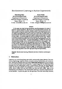
An important challenge a decision maker (DM) often face is deciding when to intervene so as to alter or prevent the progression of a condition. Instances of this challenge abound. In health service, for example, physicians are often faced with decisions about medical interventions when precipitating events threaten patients life or when patients wellbeing is severely affected[1, 12, 17]. The challenge typically requires the DM to choose between two actions i) ‘watchful waiting’ i.e. postpone the decision up to a critical point, and ii) ‘intervene’. While seemingly straightforward, such tasks (referred to as intervention timing tasks) involve uncertainty, complexity and dynamic change. We apply the power priors approach to learning a simplified abstraction of the intervention timing task I that we formulate as an MDP with unknown transition probabilities. The states of I comprise of an intervention state 0 and health states 1, 2, . . . , H + 1 in order of decreasing health (see figure (1)). The action space consists of {watchful waiting labelled w, intervene labelled i }.

Figure 1: A simplified MDP model of the intervention timing task. Transitions under watchful waiting actions are shown as solid lines while those for intervene actions are shown in broken lines. Not all possible transitions are shown in the figure. The transition probabilities for I under the watchful waiting action is of increasing failure rate (IFR). After Barlow and Proschan[2], the transition probability matrix P w is said to be IFR if the PH+1 rows of P w are increasing stochastic order, that is, s0 =i pw ss0 is monotonically increasing in s for i = 1, . . . , H + 1. The transition probabilities pw from the health states 1 ≤ s ≤ H + 1 to the s0 5

intervention state is zero under the watchful waiting action. The transition probabilities pis0 from the health states 1 ≤ s ≤ H + 1 to the intervention state is 1 under the intervene action. States 0 and i H + 1 are terminating states. The reward function rss 0 is non-negative and monotone decreasing w in s. The reward function rss0 is monotone decreasing in s. The objective is to find a policy that optimises the expected discounted total reward. In the experiments, we set H to 48 and assume that the non-zero transition probabilities pw ss0 1 ≤ −1 s, s0 ≤ H + 1 are given by pw , s ≤ s0 ≤ H + 1. This means that when the ss0 = (H + 1 − s) process is in state s then the next state is uniformly distributed in the set {s, s + 1, . . . , H + 1}. PH+1 H+1−max(i,s) These probabilities satisfy the IFR condition since, the IFR quantity s0 =i pw is ss0 = H+1−s0 monotonically increasing in s for i = 1, . . . , H + 1. The IFR quantity for the experimental settings is shown in Figure 2.

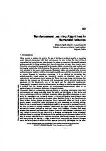
Figure 2: IFR setting for the numerical example

Figure 3: Plot of discounted total rewards over time for scenarios 1 (non informative prior) and 2 (noninformative prior + historical data) of the intervention timing task compared to optimal policy.

We use an optimistic model selection (OMS) algorithm [23] to obtain value estimates. Performance of the learning agent can be measured in several ways. To account for exploration and exploitation trade-off we measured the discounted total reward to-go at each point at each time step. More precisely, suppose the agent receives the following rewards r1 , r2 , . . . , rt in a run of time length t. P 0 The reward to go at time t0 is defined to be t0 ≥t rt 0 γ (t −t) . We experiment with two learning scenarios. In scenario 1, we assume that there is no historical data and prior distribution is non-informative with every entry of M set to 0 except for transitions to an imaginary state whose observation counts were set to 1. In scenario 2 we assume that historical data is available alongside the non-informative prior distribution of scenario 1. We draw 500 samples from the actual transition probability of I to form the historical data. For scenario 2, we used a Beta distribution (ρ = 1 in equation (13) ) to model δ with a fixed set of parameters αδ = 5 and βδ = 1. We set γ to 0.99. The results of the experiments are illustrated in Figure 3 showing the first 300 time steps. The results (average of 20 runs, 5000 trials) show that, with the δ settings used in scenario 2, the power prior approach resulted in an improvement over the performance obtained in scenario 1.

5

Conclusions

We studied in this paper the use of power priors in reinforcement learning as an approach for incorporating external evidence in the form of historical data. The main driver for the power prior approach is its relative precision parameter that weighs the external evidence relative to the likelihood of the current task. Numerical example shown in this paper indicates that the power priors approach does improve learning performance. Further work is required to quantify the gains from using power priors in Bayesian reinforcement learning. How to effectively establish an optimal setting for the precision parameter is an outstanding issue that is subject of future work. In addition, important areas of future work concerns how structural properties of a new task impacts on the precision parameter. Finally, when there are multiple historical data sets, it is possible to incorporate the whole of the historical data sets in power priors by generalising the approach we described above for single historical data. 6

References [1] A LAGOZ , O., M AILLART, L. M., S CHAEFER , A. J., AND ROBERTS , M. S. The Optimal Timing of Living-Donor Liver Transplantation. Management Science 50, 10 (2004), 1420–1430. [2] BARLOW, R. E., York, 1965.

AND

P ROSCHAN , F. Mathematical Theory of Reliability. John Wiley and Sons, New

[3] B ELLMAN , R. E. Adaptive control processes: A guided tour. Princeton University Press, 1961. [4] C HEN , M. H., I BRAHIM , J. G., AND S HAO , Q. M. Power prior distributions for generalized linear models. Journal of Statistical Planning and Inference 84 (2000), 121–137. [5] D IACONIS , P., AND Y LVISAKER , D. Conjugate priors for exponential families. Annals of Statistics 7 (1979), 269–281. [6] D UAN , Y. A Modified Bayesian Power Prior Approach with Applications in Water Quality Evaluation. PhD thesis, Faculty of Virginia Polytechnic Institute and State University, Blacksburg, Virginia, 2005. [7] I BRAHIM , J. G., AND C HEN , M. H. Power prior distributions for regression models. Statistical Science 15 (2000), 46–60. [8] I BRAHIM , J. G., C HEN , M. H., AND S INHA , D. Bayesian Survival analysis. Springer Series in Statistics, New York Heidelberg Berlin, 2002. [9] I BRAHIM , J. G., C HEN , M. H., AND S INHA , D. On optimality properties of the power prior. Journal of the American Statistical Association 98 (2003), 204–213. ´ Y´ , M., K HAILOVA , N., N EDOMA , P., AND B OHM ¨ [10] K ARN , J. Quantification of prior information revised. International Journal of Adaptive Control and Signal Processing (2001). [11] L AZARIC , A., R ESTELLI , M., AND B ONARINI , A. Transfer of Samples in Batch Reinforcement Learning. International Conference on Machine Learning (ICML) (2008). [12] M AGNI , P., Q UAGLINI , S., M ARCHETTI , M., AND BAROSI , G. Deciding when to intervene: a Markov decision process approach. International Journal of Medical Informatics 50 (2000), 237–253. [13] M ARTIN , J. Bayesian decision problems and Markov chains. Wiley, New York, 1967. [14] M ORRIS , C. N. Natural exponential families with quadratic variance functions: statistical theory. Annals of Statistics 11 (1983), 515–529. [15] N EAL , R. M. Transferring prior information between models using imaginary data. Tech. rep., University of Toronto, Toronto, Ontario, Canada, 2001. [16] P OUPART, P., V LASSIS , N., H OEY, J., AND R EGAN , K. An analytic solution to discrete Bayesian reinforcement learning. In ICML ’06: Proceedings of the 23rd International Conference on Machine learning (New York, NY, USA, 2006), ACM, pp. 697–704. [17] S HECHTER , S. M., BAILEY, M. D., S CHAEFER , A. J., AND ROBERTS , M. S. The optimal time to initiate hiv therapy under ordered health states. Operations Research 56, 1 (2007), 20–33. [18] S PIEGELHALTER , D. J., A BRAMS , K. R., AND M YLES , J. P. Bayesian Approaches to Clinical Trials and Health-care Evaluation. Chichester England: John Wiley & Sons, 2004. [19] S TRENS , M. A Bayesian framework for reinforcement learning. In ICML ’00: Proceedings of the Seventeenth International Conference on Machine Learning (2000), Stanford University, pp. 943–950. [20] S UNMOLA , F. T., AND W YATT, J. L. Model transfer for Markov decision tasks via parameter matching. Workshop of the UK Planning and Scheduling Special Interest Group (2006). [21] TAYLOR , M. E., J ONG , N. K., AND S TONE , P. Transferring Instances for Model-Based Reinforcement Learning. In The European Conference on Machine Learning & Principles and Practice of Knowledge Discovery in Databases ECML- PKDD (September 2008), Antwerp, Belgium. [22] T ESAR , L. Processing of prior information as function of data. Tech. rep., Institute of Information Theory and Automation Academy of Sciences of the Czech Republic, 2004. [23] W YATT, J. L. Exploration control in reinforcement learning using optimistic model selection. In ICML ’01: International Conference on Machine Learning (2001), A. Danyluk and C. Brodley, Eds.

7