tutorial. In practical terms, this means that we can walk the Markov chain, occasionally outputting samples, and that ..
Incorporating Non-local Information into Information Extraction Systems by Gibbs Sampling Jenny Rose Finkel, Trond Grenager, and Christopher Manning Computer Science Department Stanford University Stanford, CA 94305 {jrfinkel, grenager, manning}@cs.stanford.edu
Abstract Most current statistical natural language processing models use only local features so as to permit dynamic programming in inference, but this makes them unable to fully account for the long distance structure that is prevalent in language use. We show how to solve this dilemma with Gibbs sampling, a simple Monte Carlo method used to perform approximate inference in factored probabilistic models. By using simulated annealing in place of Viterbi decoding in sequence models such as HMMs, CMMs, and CRFs, it is possible to incorporate non-local structure while preserving tractable inference. We use this technique to augment an existing CRF-based information extraction system with long-distance dependency models, enforcing label consistency and extraction template consistency constraints. This technique results in an error reduction of up to 9% over state-of-the-art systems on two established information extraction tasks.
1 Introduction Most statistical models currently used in natural language processing represent only local structure. Although this constraint is critical in enabling tractable model inference, it is a key limitation in many tasks, since natural language contains a great deal of nonlocal structure. A general method for solving this problem is to relax the requirement of exact inference, substituting approximate inference algorithms instead, thereby permitting tractable inference in models with non-local structure. One such algorithm is Gibbs sampling, a simple Monte Carlo algorithm that is appropriate for inference in any factored probabilistic model, including sequence models and probabilistic context free grammars (Geman and Geman, 1984). Although Gibbs sampling is widely used elsewhere, there has been extremely little use
of it in natural language processing.1 Here, we use it to add non-local dependencies to sequence models for information extraction. Statistical hidden state sequence models, such as Hidden Markov Models (HMMs) (Leek, 1997; Freitag and McCallum, 1999), Conditional Markov Models (CMMs) (Borthwick, 1999), and Conditional Random Fields (CRFs) (Lafferty et al., 2001) are a prominent recent approach to information extraction tasks. These models all encode the Markov property: decisions about the state at a particular position in the sequence can depend only on a small local window. It is this property which allows tractable computation: the Viterbi, Forward Backward, and Clique Calibration algorithms all become intractable without it. However, information extraction tasks can benefit from modeling non-local structure. As an example, several authors (see Section 8) mention the value of enforcing label consistency in named entity recognition (NER) tasks. In the example given in Figure 1, the second occurrence of the token Tanjug is mislabeled by our CRF-based statistical NER system, because by looking only at local evidence it is unclear whether it is a person or organization. The first occurrence of Tanjug provides ample evidence that it is an organization, however, and by enforcing label consistency the system should be able to get it right. We show how to incorporate constraints of this form into a CRF model by using Gibbs sampling instead of the Viterbi algorithm as our inference procedure, and demonstrate that this technique yields significant improvements on two established IE tasks. 1 Prior uses in NLP of which we are aware include: Kim et
al. (1995), Della Pietra et al. (1997) and Abney (1997).
the
news
agency
Tanjug
reported
...
airport
,
Tanjug
said
.
Figure 1: An example of the label consistency problem excerpted from a document in the CoNLL 2003 English dataset.
2 Gibbs Sampling for Inference in Sequence Models In hidden state sequence models such as HMMs, CMMs, and CRFs, it is standard to use the Viterbi algorithm, a dynamic programming algorithm, to infer the most likely hidden state sequence given the input and the model (see, e.g., Rabiner (1989)). Although this is the only tractable method for exact computation, there are other methods for computing an approximate solution. Monte Carlo methods are a simple and effective class of methods for approximate inference based on sampling. Imagine we have a hidden state sequence model which defines a probability distribution over state sequences conditioned on any given input. With such a model M we should be able to compute the conditional probability P M (s|o) of any state sequence s = {s0 , . . . , s N } given some observed input sequence o = {o0 , . . . , o N }. One can then sample sequences from the conditional distribution defined by the model. These samples are likely to be in high probability areas, increasing our chances of finding the maximum. The challenge is how to sample sequences efficiently from the conditional distribution defined by the model. Gibbs sampling provides a clever solution (Geman and Geman, 1984). Gibbs sampling defines a Markov chain in the space of possible variable assignments (in this case, hidden state sequences) such that the stationary distribution of the Markov chain is the joint distribution over the variables. Thus it is called a Markov Chain Monte Carlo (MCMC) method; see Andrieu et al. (2003) for a good MCMC tutorial. In practical terms, this means that we can walk the Markov chain, occasionally outputting samples, and that these samples are guaranteed to be drawn from the target distribution. Furthermore, the chain is defined in very simple terms: from each state sequence we can only transition to a state se-
quence obtained by changing the state at any one position i, and the distribution over these possible transitions is just PG (s(t ) |s(t −1)) = P M (si(t ) |s(t−i−1) , o).
(1)
where s−i is all states except si . In other words, the transition probability of the Markov chain is the conditional distribution of the label at the position given the rest of the sequence. This quantity is easy to compute in any Markov sequence model, including HMMs, CMMs, and CRFs. One easy way to walk the Markov chain is to loop through the positions i from 1 to N , and for each one, to resample the hidden state at that position from the distribution given in Equation 1. By outputting complete sequences at regular intervals (such as after resampling all N positions), we can sample sequences from the conditional distribution defined by the model. This is still a gravely inefficient process, however. Random sampling may be a good way to estimate the shape of a probability distribution, but it is not an efficient way to do what we want: find the maximum. However, we cannot just transition greedily to higher probability sequences at each step, because the space is extremely non-convex. We can, however, borrow a technique from the study of non-convex optimization and use simulated annealing (Kirkpatrick et al., 1983). Geman and Geman (1984) show that it is easy to modify a Gibbs Markov chain to do annealing; at time t we replace the distribution in (1) with P M (si(t ) |s(t−i−1), o)1/ct P A (s(t ) |s(t −1)) = P (t ) (t −1) 1/ct j P M (s j |s− j , o)
(2)
where c = {c0 , . . . , cT } defines a cooling schedule. At each step, we raise each value in the conditional distribution to an exponent and renormalize before sampling from it. Note that when c = 1 the distribution is unchanged, and as c → 0 the distribution
Inference Viterbi Gibbs Sampling
Mean Std. Dev.
CoNLL 85.51 85.54 85.51 85.49 85.51 85.51 85.51 85.51 85.51 85.51 85.51 0.01
Seminars 91.85 91.85 91.85 91.85 91.85 91.85 91.85 91.85 91.85 91.86 91.85 0.004
Table 1: An illustration of the effectiveness of Gibbs sampling, compared to Viterbi inference, for the two tasks addressed in this paper: the CoNLL named entity recognition task, and the CMU Seminar Announcements information extraction task. We show 10 runs of Gibbs sampling in the same CRF model that was used for Viterbi. For each run the sampler was initialized to a random sequence, and used a linear annealing schedule that sampled the complete sequence 1000 times. CoNLL performance is measured as per-entity F1 , and CMU Seminar Announcements performance is measured as per-token F1 .
becomes sharper, and when c = 0 the distribution places all of its mass on the maximal outcome, having the effect that the Markov chain always climbs uphill. Thus if we gradually decrease c from 1 to 0, the Markov chain increasingly tends to go uphill. This annealing technique has been shown to be an effective technique for stochastic optimization (Laarhoven and Arts, 1987). To verify the effectiveness of Gibbs sampling and simulated annealing as an inference technique for hidden state sequence models, we compare Gibbs and Viterbi inference methods for a basic CRF, without the addition of any non-local model. The results, given in Table 1, show that if the Gibbs sampler is run long enough, its accuracy is the same as a Viterbi decoder.
3 A Conditional Random Field Model Our basic CRF model follows that of Lafferty et al. (2001). We choose a CRF because it represents the state of the art in sequence modeling, allowing both discriminative training and the bi-directional flow of probabilistic information across the sequence. A CRF is a conditional sequence model which represents the probability of a hidden state sequence given some observations. In order to facilitate obtaining the conditional probabilities we need for Gibbs sampling, we generalize the CRF model in a
Feature Current Word Previous Word Next Word Current Word Character n-gram Current POS Tag Surrounding POS Tag Sequence Current Word Shape Surrounding Word Shape Sequence Presence of Word in Left Window Presence of Word in Right Window
NER
TF
X X X
X X X
all
length ≤ 6
X X X X
X X
size 4 size 4
size 9 size 9
Table 2: Features used by the CRF for the two tasks: named entity recognition (NER) and template filling (TF).
way that is consistent with the Markov Network literature (see Cowell et al. (1999)): we create a linear chain of cliques, where each clique, c, represents the probabilistic relationship between an adjacent pair of states2 using a clique potential φc , which is just a table containing a value for each possible state assignment. The table is not a true probability distribution, as it only accounts for local interactions within the clique. The clique potentials themselves are defined in terms of exponential models conditioned on features of the observation sequence, and must be instantiated for each new observation sequence. The sequence of potentials in the clique chain then defines the probability of a state sequence (given the observation sequence) as PCRF (s|o) ∝
N Y
φi (si−1 , si )
(3)
i=1
where φi (si−1 , si ) is the element of the clique potential at position i corresponding to states si−1 and si .3 Although a full treatment of CRF training is beyond the scope of this paper (our technique assumes the model is already trained), we list the features used by our CRF for the two tasks we address in Table 2. During training, we regularized our exponential models with a quadratic prior and used the quasi-Newton method for parameter optimization. As is customary, we used the Viterbi algorithm to infer the most likely state sequence in a CRF. The clique potentials of the CRF, instantiated for some observation sequence, can be used to easily 2 CRFs with larger cliques are also possible, in which case the potentials represent the relationship between a subsequence of k adjacent states, and contain |S|k elements. 3 To handle the start condition properly, imagine also that we define a distinguished start state s0 .
compute the conditional distribution over states at a position given in Equation 1. Recall that at position i we want to condition on the states in the rest of the sequence. The state at this position can be influenced by any other state that it shares a clique with; in particular, when the clique size is 2, there are 2 such cliques. In this case the Markov blanket of the state (the minimal set of states that renders a state conditionally independent of all other states) consists of the two neighboring states and the observation sequence, all of which are observed. The conditional distribution at position i can then be computed simply as PCRF (si |s−i , o) ∝ φi (si−1 , si )φi+1 (si , si+1 )
(4)
where the factor tables F in the clique chain are already conditioned on the observation sequence.
4.2
The CMU Seminar Announcements Task
This dataset was developed as part of Dayne Freitag’s dissertation research Freitag (1998).5 It consists of 485 emails containing seminar announcements at Carnegie Mellon University. It is annotated for four fields: speaker, location, start time, and end time. Sutton and McCallum (2004) used 5-fold cross validation when evaluating on this dataset, so we obtained and used their data splits, so that results can be properly compared. Because the entire dataset is used for testing, there is no development set. We also used their evaluation metric, which is slightly different from the method for CoNLL data. Instead of evaluating precision and recall on a per-entity basis, they are evaluated on a per-token basis. Then, to calculate the overall F1 score, the F1 scores for each class are averaged.
4 Datasets and Evaluation
5 Models of Non-local Structure
We test the effectiveness of our technique on two established datasets: the CoNLL 2003 English named entity recognition dataset, and the CMU Seminar Announcements information extraction dataset.
Our models of non-local structure are themselves just sequence models, defining a probability distribution over all possible state sequences. It is possible to flexibly model various forms of constraints in a way that is sensitive to the linguistic structure of the data (e.g., one can go beyond imposing just exact identity conditions). One could imagine many ways of defining such models; for simplicity we use the form Y #(λ,s,o) P M (s|o) ∝ θλ (5)
4.1
The CoNLL NER Task
This dataset was created for the shared task of the Seventh Conference on Computational Natural Language Learning (CoNLL),4 which concerned named entity recognition. The English data is a collection of Reuters newswire articles annotated with four entity types: person (PER), location (LOC), organization (ORG), and miscellaneous (MISC). The data is separated into a training set, a development set (testa), and a test set (testb). The training set contains 945 documents, and approximately 203,000 tokens. The development set has 216 documents and approximately 51,000 tokens, and the test set has 231 documents and approximately 46,000 tokens. We evaluate performance on this task in the manner dictated by the competition so that results can be properly compared. Precision and recall are evaluated on a per-entity basis (and combined into an F1 score). There is no partial credit; an incorrect entity boundary is penalized as both a false positive and as a false negative. 4 Available at http://cnts.uia.ac.be/conll2003/ner/.
λ∈3
where the product is over a set of violation types 3, and for each violation type λ we specify a penalty parameter θλ . The exponent #(λ, s, o) is the count of the number of times that the violation λ occurs in the state sequence s with respect to the observation sequence o. This has the effect of assigning sequences with more violations a lower probability. The particular violation types are defined specifically for each task, and are described in the following two sections. This model, as defined above, is not normalized, and clearly it would be expensive to do so. This doesn’t matter, however, because we only use the model for Gibbs sampling, and so only need to compute the conditional distribution at a single position i (as defined in Equation 1). One (inefficient) way 5 Available at http://nlp.shef.ac.uk/dot.kom/resources.html.
PER LOC ORG MISC
PER
LOC
ORG
MISC
3141
4 6436
5 188 2975
0 3 0 2030
Table 3: Counts of the number of times multiple occurrences of a token sequence is labeled as different entity types in the same document. Taken from the CoNLL training set.
PER LOC ORG MISC
PER
LOC
ORG
MISC
1941 0 22 14
5 167 328 224
2 6 819 7
3 63 191 365
Table 4: Counts of the number of times an entity sequence is labeled differently from an occurrence of a subsequence of it elsewhere in the document. Rows correspond to sequences, and columns to subsequences. Taken from the CoNLL training set.
to compute this quantity is to enumerate all possible sequences differing only at position i, compute the score assigned to each by the model, and renormalize. Although it seems expensive, this computation can be made very efficient with a straightforward memoization technique: at all times we maintain data structures representing the relationship between entity labels and token sequences, from which we can quickly compute counts of different types of violations. 5.1
CoNLL Consistency Model
Label consistency structure derives from the fact that within a particular document, different occurrences of a particular token sequence are unlikely to be labeled as different entity types. Although any one occurrence may be ambiguous, it is unlikely that all instances are unclear when taken together. The CoNLL training data empirically supports the strength of the label consistency constraint. Table 3 shows the counts of entity labels for each pair of identical token sequences within a document, where both are labeled as an entity. Note that inconsistent labelings are very rare.6 In addition, we also want to model subsequence constraints: having seen Geoff Woods earlier in a document as a person is a good indicator that a subsequent occurrence of 6 A notable exception is the labeling of the same text as both
organization and location within the same document. This is a consequence of the large portion of sports news in the CoNLL dataset, so that city names are often also team names.
Woods should also be labeled as a person. However, if we examine all cases of the labelings of other occurrences of subsequences of a labeled entity, we find that the consistency constraint does not hold nearly so strictly in this case. As an example, one document contains references to both The China Daily, a newspaper, and China, the country. Counts of subsequence labelings within a document are listed in Table 4. Note that there are many offdiagonal entries: the China Daily case is the most common, occurring 328 times in the dataset. The penalties used in the long distance constraint model for CoNLL are the Empirical Bayes estimates taken directly from the data (Tables 3 and 4), except that we change counts of 0 to be 1, so that the distribution remains positive. So the estimate of a PER 5 also being an ORG is 3151 ; there were 5 instance of an entity being labeled as both, PER appeared 3150 times in the data, and we add 1 to this for smoothing, because PER-MISC never occured. However, when we have a phrase labeled differently in two different places, continuing with the PER-ORG example, it is unclear if we should penalize it as PER that is also an ORG or an ORG that is also a PER. To deal with this, we multiply the square roots of each estimate together to form the penalty term. The penalty term is then multiplied in a number of times equal to the length of the offending entity; this is meant to “encourage” the entity to shrink.7 For example, say we have a document with three entities, Rotor Volgograd twice, once labeled as PER and once as ORG, and Rotor, labeled as an ORG. The likelihood of a 5 PER also being an ORG is 3151 , and of an ORG also 5 being a PER is 3169 , so the penalty for this violation q q 5 5 2 is ( 3151 × 3151 ) . The likelihood of a ORG be2 ing a subphrase of a PER is 842 . So the total penalty 5 2 5 would be 3151 × 3169 × 842 .
5.2
CMU Seminar Announcements Consistency Model
Due to the lack of a development set, our consistency model for the CMU Seminar Announcements is much simpler than the CoNLL model, the numbers where selected due to our intuitions, and we did not spend much time hand optimizing the model. 7 While there is no theoretical justification for this, we found
it to work well in practice.
Specifically, we had three constraints. The first is that all entities labeled as start time are normalized, and are penalized if they are inconsistent. The second is a corresponding constraint for end times. The last constraint attempts to consistently label the speakers. If a phrase is labeled as a speaker, we assume that the last word is the speaker’s last name, and we penalize for each occurrance of that word which is not also labeled speaker. For the start and end times the penalty is multiplied in based on how many words are in the entity. For the speaker, the penalty is only multiplied in once. We used a hand selected penalty of exp(−4.0).
6 Combining Sequence Models In the previous section we defined two models of non-local structure. Now we would like to incorporate them into the local model (in our case, the trained CRF), and use Gibbs sampling to find the most likely state sequence. Because both the trained CRF and the non-local models are themselves sequence models, we simply combine the two models into a factored sequence model of the following form P F (s|o) ∝ P M (s|o)P L (s|o) (6) where M is the local CRF model, L is the new nonlocal model, and F is the factored model.8 In this form, the probability again looks difficult to compute (because of the normalizing factor, a sum over all hidden state sequences of length N ). However, since we are only using the model for Gibbs sampling, we never need to compute the distribution explicitly. Instead, we need only the conditional probability of each position in the sequence, which can be computed as P F (si |s−i , o) ∝ P M (si |s−i , o)P L (si |s−i , o).
(7)
At inference time, we then sample from the Markov chain defined by this transition probability.
7 Results and Discussion In our experiments we compare the impact of adding the non-local models with Gibbs sampling to our 8 This model double-generates the state sequence conditioned on the observations. In practice we don’t find this to be a problem.
CoNLL Approach B & M LT- RMN B & M GLT- RMN Local+Viterbi NonLoc+Gibbs
LOC
ORG
MISC
PER
ALL
– – 88.16 88.51
– – 80.83 81.72
– – 78.51 80.43
– – 90.36 92.29
80.09 82.30 85.51 86.86
Table 5: F1 scores of the local CRF and non-local models on the CoNLL 2003 named entity recognition dataset. We also provide the results from Bunescu and Mooney (2004) for comparison. CMU Seminar Announcements Approach STIME ETIME SPEAK LOC S & M CRF 97.5 97.5 88.3 77.3 S & M Skip- CRF 96.7 97.2 88.1 80.4 Local+Viterbi 96.67 97.36 83.39 89.98 NonLoc+Gibbs 97.11 97.89 84.16 90.00
ALL
90.2 90.6 91.85 92.29
Table 6: F1 scores of the local CRF and non-local models on the CMU Seminar Announcements dataset. We also provide the results from Sutton and McCallum (2004) for comparison.
baseline CRF implementation. In the CoNLL named entity recognition task, the non-local models increase the F1 accuracy by about 1.3%. Although such gains may appear modest, note that they are achieved relative to a near state-of-the-art NER system: the winner of the CoNLL English task reported an F1 score of 88.76. In contrast, the increases published by Bunescu and Mooney (2004) are relative to a baseline system which scores only 80.9% on the same task. Our performance is similar on the CMU Seminar Announcements dataset. We show the per-field F1 results that were reported by Sutton and McCallum (2004) for comparison, and note that we are again achieving gains against a more competitive baseline system. For all experiments involving Gibbs sampling, we used a linear cooling schedule. For the CoNLL dataset we collected 200 samples per trial, and for the CMU Seminar Announcements we collected 100 samples. We report the average of all trials, and in all cases we outperform the baseline with greater than 95% confidence, using the standard t-test. The trials had low standard deviations – 0.083% and 0.007% – and high minimun F-scores – 86.72%, and 92.28% – for the CoNLL and CMU Seminar Announcements respectively, demonstrating the stability of our method. The biggest drawback to our model is the computational cost. Taking 100 samples dramatically increases test time. Averaged over 3 runs on both
Viterbi and Gibbs, CoNLL testing time increased from 55 to 1738 seconds, and CMU Seminar Announcements testing time increases from 189 to 6436 seconds.
8 Related Work Several authors have successfully incorporated a label consistency constraint into probabilistic sequence model named entity recognition systems. Mikheev et al. (1999) and Finkel et al. (2004) incorporate label consistency information by using adhoc multi-stage labeling procedures that are effective but special-purpose. Malouf (2002) and Curran and Clark (2003) condition the label of a token at a particular position on the label of the most recent previous instance of that same token in a prior sentence of the same document. Note that this violates the Markov property, but is achieved by slightly relaxing the requirement of exact inference. Instead of finding the maximum likelihood sequence over the entire document, they classify one sentence at a time, allowing them to condition on the maximum likelihood sequence of previous sentences. This approach is quite effective for enforcing label consistency in many NLP tasks, however, it permits a forward flow of information only, which is not sufficient for all cases of interest. Chieu and Ng (2002) propose a solution to this problem: for each token, they define additional features taken from other occurrences of the same token in the document. This approach has the added advantage of allowing the training procedure to automatically learn good weightings for these “global” features relative to the local ones. However, this approach cannot easily be extended to incorporate other types of non-local structure. The most relevant prior works are Bunescu and Mooney (2004), who use a Relational Markov Network (RMN) (Taskar et al., 2002) to explicitly models long-distance dependencies, and Sutton and McCallum (2004), who introduce skip-chain CRFs, which maintain the underlying CRF sequence model (which (Bunescu and Mooney, 2004) lack) while adding skip edges between distant nodes. Unfortunately, in the RMN model, the dependencies must be defined in the model structure before doing any inference, and so the authors use crude heuristic
part-of-speech patterns, and then add dependencies between these text spans using clique templates. This generates a extremely large number of overlapping candidate entities, which then necessitates additional templates to enforce the constraint that text subsequences cannot both be different entities, something that is more naturally modeled by a CRF. Another disadvantage of this approach is that it uses loopy belief propagation and a voted perceptron for approximate learning and inference – ill-founded and inherently unstable algorithms which are noted by the authors to have caused convergence problems. In the skip-chain CRFs model, the decision of which nodes to connect is also made heuristically, and because the authors focus on named entity recognition, they chose to connect all pairs of identical capitalized words. They also utilize loopy belief propagation for approximate learning and inference. While the technique we propose is similar mathematically and in spirit to the above approaches, it differs in some important ways. Our model is implemented by adding additional constraints into the model at inference time, and does not require the preprocessing step necessary in the two previously mentioned works. This allows for a broader class of long-distance dependencies, because we do not need to make any initial assumptions about which nodes should be connected, and is helpful when you wish to model relationships between nodes which are the same class, but may not be similar in any other way. For instance, in the CMU Seminar Announcements dataset, we can normalize all entities labeled as a start time and penalize the model if multiple, nonconsistent times are labeled. This type of constraint cannot be modeled in an RMN or a skip-CRF, because it requires the knowledge that both entities are given the same class label. We also allow dependencies between multi-word phrases, and not just single words. Additionally, our model can be applied on top of a pre-existing trained sequence model. As such, our method does not require complex training procedures, and can instead leverage all of the established methods for training high accuracy sequence models. It can indeed be used in conjunction with any statistical hidden state sequence model: HMMs, CMMs, CRFs, or even heuristic models. Third, our technique employs Gibbs sampling for approximate inference, a simple
and probabilistically well-founded algorithm. As a consequence of these differences, our approach is easier to understand, implement, and adapt to new applications.
9 Conclusions We have shown that a constraint model can be effectively combined with an existing sequence model in a factored architecture to successfully impose various sorts of long distance constraints. Our model generalizes naturally to other statistical models and other tasks. In particular, it could in the future be applied to statistical parsing. Statistical context free grammars provide another example of statistical models which are restricted to limiting local structure, and which could benefit from modeling nonlocal structure.
Acknowledgements This work was supported in part by the Advanced Research and Development Activity (ARDA)’s Advanced Question Answering for Intelligence (AQUAINT) Program. Additionally, we would like to thank our reviewers for their helpful comments.
References S. Abney. 1997. Stochastic attribute-value grammars. Computational Linguistics, 23:597–618. C. Andrieu, N. de Freitas, A. Doucet, and M. I. Jordan. 2003. An introduction to MCMC for machine learning. Machine Learning, 50:5–43. A. Borthwick. 1999. A Maximum Entropy Approach to Named Entity Recognition. Ph.D. thesis, New York University. R. Bunescu and R. J. Mooney. 2004. Collective information extraction with relational Markov networks. In Proceedings of the 42nd ACL, pages 439–446. H. L. Chieu and H. T. Ng. 2002. Named entity recognition: a maximum entropy approach using global information. In Proceedings of the 19th Coling, pages 190–196. R. G. Cowell, A. Philip Dawid, S. L. Lauritzen, and D. J. Spiegelhalter. 1999. Probabilistic Networks and Expert Systems. Springer-Verlag, New York. J. R. Curran and S. Clark. 2003. Language independent NER using a maximum entropy tagger. In Proceedings of the 7th CoNLL, pages 164–167. S. Della Pietra, V. Della Pietra, and J. Lafferty. 1997. Inducing features of random fields. IEEE Transactions on Pattern Analysis and Machine Intelligence, 19:380–393. J. Finkel, S. Dingare, H. Nguyen, M. Nissim, and C. D. Manning. 2004. Exploiting context for biomedical entity recognition: from syntax to the web. In Joint Workshop on Natural Language Processing in Biomedicine and Its Applications at Coling 2004.
D. Freitag and A. McCallum. 1999. Information extraction with HMMs and shrinkage. In Proceedings of the AAAI-99 Workshop on Machine Learning for Information Extraction. D. Freitag. 1998. Machine learning for information extraction in informal domains. Ph.D. thesis, Carnegie Mellon University. S. Geman and D. Geman. 1984. Stochastic relaxation, Gibbs distributions, and the Bayesian restoration of images. IEEE Transitions on Pattern Analysis and Machine Intelligence, 6:721–741. M. Kim, Y. S. Han, and K. Choi. 1995. Collocation map for overcoming data sparseness. In Proceedings of the 7th EACL, pages 53–59. S. Kirkpatrick, C. D. Gelatt, and M. P. Vecchi. 1983. Optimization by simulated annealing. Science, 220:671–680. P. J. Van Laarhoven and E. H. L. Arts. 1987. Simulated Annealing: Theory and Applications. Reidel Publishers. J. Lafferty, A. McCallum, and F. Pereira. 2001. Conditional Random Fields: Probabilistic models for segmenting and labeling sequence data. In Proceedings of the 18th ICML, pages 282–289. Morgan Kaufmann, San Francisco, CA. T. R. Leek. 1997. Information extraction using hidden Markov models. Master’s thesis, U.C. San Diego. R. Malouf. 2002. Markov models for language-independent named entity recognition. In Proceedings of the 6th CoNLL, pages 187–190. A. Mikheev, M. Moens, and C. Grover. 1999. Named entity recognition without gazetteers. In Proceedings of the 9th EACL, pages 1–8. L. R. Rabiner. 1989. A tutorial on Hidden Markov Models and selected applications in speech recognition. Proceedings of the IEEE, 77(2):257–286. C. Sutton and A. McCallum. 2004. Collective segmentation and labeling of distant entities in information extraction. In ICML Workshop on Statistical Relational Learning and Its connections to Other Fields. B. Taskar, P. Abbeel, and D. Koller. 2002. Discriminative probabilistic models for relational data. In Proceedings of the 18th Conference on Uncertianty in Artificial Intelligence (UAI-02), pages 485–494, Edmonton, Canada.