Incorporating Prior Information in Machine Learning by ... - CiteSeerX

Incorporating Prior Information in Machine Learning by Creating Virtual Examples P. Niyogi, F. Girosi, and T. Poggio MIT Center for Biological and Computational Learning Cambridge, MA 02139. September 2, 1998

Abstract

One of the key problems in supervised learning is the insucient size of the training set. The natural way for an intelligent learner to counter this problem and successfully generalize is to exploit prior information that may be available about the domain or that can be learned from prototypical examples. We discuss the notion of using prior knowledge by creating virtual examples and thereby expanding the eective training set size. We show that in some contexts, this idea is mathematically equivalent to incorporating the prior knowledge as a regularizer, suggesting that the strategy is well-motivated. The process of creating virtual examples in real world pattern recognition tasks is highly non-trivial. We provide demonstrative examples from object recognition and speech recognition to illustrate the idea.

1

1 Learning from Examples Recently, machine learning techniques have become increasingly popular as an alternative to knowledge-based approaches to arti cial intelligence problems in a variety of elds. The hope is that automatic learning from examples will eliminate the need for laborious handcrafting of domain-speci c knowledge about the task at hand. However, analyses of the complexity of learning problems suggest that this hope might be overly optimistic | often the number of examples needed to solve the problem might be prohibitive. Clearly, a middle ground is needed and a useful direction of research is the study of how to incorporate prior world knowledge of the task within a learning from examples framework. The current paper deals with this subject. We rst begin by providing some background about how the problem of learning from examples is usually formulated. In the next section, we discuss brie y the complexity of the learning problem and why, in the absence of any prior knowledge, one might require a large number of examples to learn well. In section 3, we introduce the idea of virtual examples, i.e., creating additional examples from the current set of examples by utitilizing speci c knowledge about the task at hand. While the overall framework is similar to learning from hints (Abu-Mostafa,1995), our emphasis in this paper is to describe some speci c non-trivial transformations that allow us to create virtual examples for real world pattern recognition problems. We rst show in section 4 that in certain function learning contexts, the framework of virtual examples is equivalent to imposing prior knowledge as a regularizer. Thus, the idea of virtual examples can be more than an ad hoc strategy. We then discuss in section 5, some speci c examples from computer vision and speech recognition. Finally, we conclude by reiterating some of our main points in section 6.

1.1 Background: Learning as Function Approximation

The problem of learning from examples can be usefully modeled as trying to approximate some unknown target function f from (x; y ) pairs that are consistent with this function (modulo noise). The target function f belongs to some target class of functions denoted by F : The learner has access to a data set consisting of (say) n (x; y ) pairs ((xi; yi ) : i = 1; : : :; n) and picks a function h chosen from some hypothesis class H on the basis of this data set. The hope is that if "enough" examples are drawn, the learner's hypothesis 2

will be suciently close to the target resulting in successful generalization to novel unlabelled examples that the learner might encounter. Numerous problems in pattern recognition, speech, vision, handwriting, nance, robotics, etc. can be cast within this framework and research typically focuses on dierent kinds of hypothesis classes ( H) and dierent ways of choosing an optimal function in this class (training algorithms). Thus, multilayer perceptrons (Rumelhart, Mcllelland and Hinton, 1986), radial basis function networks (Poggio and Girosi, 1990; Moody and Darken, 1988), decision trees (Breiman etal, 1984), all correspond to dierent choices of hypothesis classes on which popular learning machines have been based. Similarly, dierent kinds of gradient descent schemes from backpropagation to the EM algorithm correspond to ways of choosing an optimal function from such a class given a nite data set. By varying the choices of hypothesis classes and training algorithms, a profusion of learning paradigms have emerged. The most signi cant issue of interest in each of these learning paradigms is how they generalize to new unseen data. In the next section, we discuss the factors upon which the generalization performance of a learning machine depends.

2 Prior Information and the Problem of Sample Complexity In any learning from examples system, the number of examples (l) that needs to be collected for successful generalization is a key issue. This sample complexity is typically characterized by the theory of Vapnik and Chervonenkis (1982,1995) that describes the general laws that all probabilistically based learning machines have to obey. It turns out that if the learner picks a hypothesis (^h 2 H) on the basis of the example set, then the of q V Cnumber ( H ) examples it needs in order to generalize well is of the order of l : Here V C (H) is the VC-dimension of the class H | a combinatorial measure of the complexity of the hypothesis class. Roughly speaking, the VC dimension (see Vapnik, 1982 for further details) is a measure of how many dierent kinds of functions there are in H: For example, if H were the parametric class of univariate polynomials of degree n; its VC dimension1 is n + 1. In While in this case, the VC dimension is related in a simple way to the number of parameters, this need not be true in general. One can think of classes with many parameters having a small VC dimension and vice versa. Thus the VC dimension is a better and more direct measure of learning complexity than simply the number of parameters. 1

3

general, large or complex hypothesis classes that can accomodate many different data sets would have a higher VC dimension than smaller, restricted hypothesis classes. Thus we see that the number of examples needed is proportional to the VC-dimension, and in this sense, to the eective size of the hypothesis class. Consequently, it is in our interest to use small hypothesis classes in learning machines. However, using a small hypothesis class is not enough. Recall that the target function f belongs to F and if our hypothesis class H is too small, then, even if we choose the best function in it, the distance from the target (generalization error) might be too high. To appreciate this point better, let us consider a situation of learning using neural networks in a least-squares setting. Recall that ideally, we would like to \learn" the target function that is given by the following (the expectation is with respect to the true probability distribution generating the data):

f0  arg min E [(y ? f (x))2] f 2F

However, in practice, we don't know the true distribution and so cannot compute the true expectation; nor do we typically minimize over the class F : For example, consider the typical situation if we were using neural networks to learn the function f0 : We draw a nite data set (x; y pairs), construct an empirical approximation to the objective function and then minimize this over a class of neural networks with a nite number of parameters. If we collected l data points and minimized over a neural network with n nodes in its hidden layer (say), we are in eect computing the following function f^n;l : l 2]  min 1 X(y ? h(x ))2 E [( y ? h ( x )) f^n;l = arg hmin i h2Hn l i=1 i 2Hn emp Thus, when we attempt to learn the function f0 using a nite amount of data (l points) and a hypothesis class with a nite number of parameters (Hn ) then, the function we obtain in practice is given by f^n;l : This is the

function we use to predict future, unknown values and naturally, we would like to know how good this function is, i.e., how far this function is from the true target. In general, one can show that the generalization error (k f0 ? f^n;l k) can be decomposed into an approximation component and an estimation component, i.e., 4

k f0 ? f^n;l k eapp(n) + eest( V C (lHn) ) The approximation error eapp(n) is due to the nite size of the hypothesis class. As the number of hidden nodes, n; increases, the representational

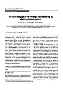
power of the hypothesis class increases and the approximation error goes to zero. The estimation error eest ( V C (lHn ) ) is due to the nite amount of data that is available to the learner. It is a monotonically decreasing function and depends upon the VC dimension of the hypothesis class Hn and the amount of data (l). As the number of hidden nodes increases, the VC dimension of Hn increases and consequently the estimation error increases as well (keeping the data xed). Thus to make the approximation error small, we need large sized networks (n large); to make the estimation error small, we need small sized networks (n small). This trade-o between the approximation error and estimation error arises in all learning paradigms and has been investigated for a number of dierent hypothesis classes ranging from multilayer perceptrons (Barron, 1994) to radial basis functions (Niyogi and Girosi, 1996). The following theorem states a canonical result for radial basis functions and g. 1 below describes the generalization error surface as a function of the number of parameters and the number of data.

Theorem 1 (Niyogi and Girosi,1996) Let Hn be the class of Gaussian

Radial Basis Function networks with k input nodes and n hidden nodes, i.e.,

Hn =

n X i=1

ciGi( xi ? ti ) i

k Let f0 be an element of the Bessel potential space2 Lm 1 (R ) of order m; with m > k=2 (the class F ). Assume that a data set f(xi; yi )gli=1 has been obtained by randomly sampling the function f0 in presence of noise, and that the noise distribution has compact support. Then, for any 0 <  < 1, with probability greater than 1 ?  , the following bound for the generalization error

This is de ned as the set of functions f that can be written as f =   Gm , where  stands for the convolution operation,  2 Lp and Gm is the Bessel-Macdonald kernel, i.e., the function whose Fourier transform is: 1 ~ m (s) = G (1 + 42 ksk2 )m=2 2

5

holds:

kf0 ? f^n;l k2L2(P )  O

1

n +O

 nk ln(nl) ? ln  1=2! l

(1)

Figure 1: The generalization error, the number of examples (l) and the number of basis functions (n) as a function of each other. What do we conclude from all this? First, that if we work with unconstrained hypothesis classes, the number of examples needed for low estimation error will almost certainly be prohibitive. On the other hand, if we work with highly constrained hypothesis classes, the approximation error will be too high for successful generalization. The only way around this dilemma is if the target class itself (F ) can be made small | but this is precisely the prior information we have about the problem being solved. Thus, if we have more prior information about the target function, it would correspond 6

to a smaller target class and the problems with poor generalization would be ameliorated. In essence, prior information is more than a good idea. The mathematics of generalization (from the no-free-lunch theorems of Wolpert (1995) to the statistical theory of Vapnik (1995)) all point to one thing | incorporation of prior knowledge might be the only way for learning machines to tractably generalize from nite data. One way of incorporating prior knowledge is the idea of virtual examples: utilizing prior information about the target function to generate novel examples from old data thereby enlarging our eective data set. We discuss this in the next section.

3 Virtual Examples: A Framework for Prior Information As we have discussed above, a signi cant problem in learning from examples is the large amount of data (examples) needed for adequate learning. Consequently, it becomes crucial to exploit any form of prior knowledge we might have about the task at hand. A well known technique for incorporating prior information is to restrict the class of hypotheses | this would also reduce the data requirements by the Vapnik Chervonenkis theory as discussed in the previous section. Another alternative might be to expand the set of available examples in some fashion so that the learner has access to an eectively larger set of examples resulting in more accurate learning. These additional examples, created from the existing ones by the application of prior knowledge, will be referred to as virtual examples ( rst introduced by Poggio and Vetter, 1992 and dierent from the notion of virtual examples introduced by Abu Mostafa (1990,1992,1993) as discussed later). We rst lay the general framework for virtual examples in section 3.1. Of course, virtual examples is only one way of incorporating prior information and we will brie y review some alternate methods and their relationship to our approach in section 3.2. At rst, the idea of virtual examples might seem like an ad-hoc one but we show in section 4 the connection between the virtual examples approach and using regularization as a technique for incorporating prior information. For the example discussed, it is possible to prove that both techniques yield the same solution. The heart of the virtual examples idea involves the actual creation of the virtual examples |- this is the main focus of our paper and we discuss several substantive real world, practical demonstrations of this 7

approach in later sections.

3.1 The General Framework

As discussed earlier, the primary goal of the learner is to approximate some unknown target function (f ) from examples ((x; y ) pairs) of this function. The unknown target function might be a real-valued, multivariate function (as in sec. 4), or even a characteristic funtion de ned over some manifold (as in sec. 5). In the absence of any prior information, the learner would attempt to t a function from H to the data set and use it to predict future values. Suppose, however, that we have prior knowledge of a set of transformations that allow us to obtain new examples from old. For example, the target function might be invariant with respect to a particular group of transformations. A simple case is when the target function is known to be even or odd. A more complex case might be if the target function is a characteristic function de ned over a manifold of 3D objects. Correspondingly, in some cases, obtaining the new examples might be easy, in other cases | as in the case for object recognition | it is quite dicult. Thus, suppose we know some transformation T such that if (x; f (x)) is a valid example, then (Tx; yT (f (x))) is also a valid example. For an invariant transformation, yT is the identity mapping. In general, of course, the relation of yT to T depends upon the prior knowledge of the problem and might be quite complex. Then, given a set of n examples: D = f(x1; y1); : : :; (xn; yn)g and knowledge of this transformation T; we generate the set of virtual examples: D0 = f(x01; y10 ); : : :; (x0n ; yn0 )g such that x0i = Tx and yi0 = yT (yi ): (x; f (x)) T;y ?!T (Tx; yT (f (x))) For many interesting cases, prior knowledge of the problem might allow us to de ne a group of transformations T such that for every T 2 T ; we can create new, virtual examples from the old data set. For example, rotations (in the image plane or in 3D) might de ne such a group for object recognition problems. Thus, the creation of virtual examples allows us to expand the example set and consequently move towards better generalization.

8

3.2 Techniques for Prior Information and Related Research Needless to say, the idea of virtual examples is only one possible way of incorporating prior information. We discuss in this section various ways in which researchers have tried to utilize prior knowledge.

1. Prior Knowledge in the Choice of Variables or Features: Prior knowledge could be used in the choice of the variables or features that are used to represent the problem. Let us consider the case of object recognition. A simple form of prior knowledge is that the rotated version (in 2D) of an object still represents that object. Therefore one could think of using, as input to the network, features that are invariant under rotations in the image plane. In this case, rotation invariant recognition would be achieved with just one example. This approach is somehow limited in vision applications, because it is very dicult to nd features that are invariant for \interesting" transformations. For example it does not seem likely that one can nd features of face images that are invariant with respect to rotation in 3D space, apart from \trivial" ones such as the colour of the person's hair etc. (for more details on the possibilities of such an approach, see Mundy et al, 1992). Another kind of prior knowledge could be that certain features always appear in conjunction (or disjunction), or certain variables are always linked together in a certain form. In this case one could explicitly add these new variables to the set of original variables, making the learning task much easier. For example, in robotics it is known that for certain mechanical systems, the relation between torques and state variables is represented by certain combinations of trigonometric functions. Therefore, explicitly adding sine and cosine transformation of the state space variables usually makes the problem much easier to solve. This technique is also not uncommon in statistics, where often new variables are created by means of nonlinear transformation of the original ones. 2. Prior Knowledge in the Learning Technique: Another way to incorporate prior knowledge is to embed it in the learning technique. Examples of this are the recent transformation distance technique introduced by Simard, Le Cun and Denker (1993). The idea underlying this technique is the following: suppose a pattern classi cation 9

problem has to be solved, and we know that the outcome of the classi cation scheme should be invariant with respect to a certain transformation R(w), where w is a set of parameters (for example the rotation angle in the image plane for object recognition). This means that for every input pattern x there is a manifold S x on which the output should be constant. Therefore, if we desire to use a classi cation technique such as Nearest Neighbors, that is based on a notion of distance, we should use as distance between two patterns x and z not the Euclidean distance between them, but the Euclidean distance between the manifolds S (x) and S (z). This quantity cannot be computed analytically, in general, but Simard, Le Cun and Denker (1993) show how to estimate it using a local approximation of the manifold S (x) by its tangent plane that can be experimentally computed. In this case the prior knowledge has been embedded in the de nition of distance, and therefore in the learning technique, rather than in the choice of the variables, as described above. Another case in which prior knowledge is embedded in the learning technique is regularization theory, a set of mathematical tools introduced by Tikhonov in order to deal with ill-posed problems (Tikhonov, 1963; Tikhonov and Arsenin, 1977; Morozov, 1984; Bertero, 1986; Wahba, 1990; Poggio and Girosi, 1990; Girosi, Jones and Poggio, 1995). In regularization theory an ill-posed problem is transformed into a well-posed one using some prior knowledge. The most common form of prior knowledge is smoothness, whose role in the theory of learning from examples has been investigated at length by Poggio and Girosi (1990). However, other forms of prior knowledge can be used in the framework of regularization theory. This topic has been investigated by Verri and Poggio (1986), who gave sucient conditions for a constraint to be embedded in the regularization framework. Examples of the prior knowledge they considered include monotonicity, convexity and positivity. 3. Generating New Examples with Prior Knowledge: Another form of utilising prior knowledge for learning is the idea of generating new examples from the existing data set. This is the idea of virtual examples (from Poggio and Vetter, 1992) that we consider in this paper. An example of a similar technique can be found in the work of Pomerleau (1989, 1991) on ALVINN, an autonomous navigation vehicle that learns to drive on a highway. The system consists of a camera mounted 10

on a vehicle, and a neural network that takes that the image of the road as an input and produces as output a set of steering commands. The examples are acquired by recording the actions of a human driver. Since humans are very good at keeping the vehicle in the right lane, the images of the road look all alike, and there are no examples of what action to take if the vehicle is in an \unusual attitude", that is, too far to the right or to the left. Therefore the network is not able to give correct answers if it nds itself in these kinds of situations, of which it has no examples. Pomerleau used prior knowledge on the geometry of the problem in order to create examples of what to do in the case of unusual attitudes. Knowing the location of the camera, with respect to the vehicle, and based on examples belonging to the data set created by the human driver, he was able to create images of what the road would look like if the vehicle were in an unusual attitude, say too close to the centerline. Given these new images and the corresponding locations of the vehicle he computed what the steering command should be for each one of them, creating a whole new set of images, now containing many examples of unusual attitudes, and allowing the system to achieve excellent performance. 4. Incorporating Prior Knowledge as Hints: Another technique is the one proposed by Abu-Mostafa (1990, 1992, 1993). Here we list very brie y the main points of his concept of hints. The approach overlaps to a good extent but not completely with our own ideas of virtual examples. Consider (a) a function f to be learned with domain, X; and range, Y ; (b) the hypothesis g provided by the learning process, say by a Regularization Network approximation of f ; (c) the functional E (g; f ) measuring the error. Then a hint Hm is a test that f must satisfy. One generates one example of the hint and measures em , the amount of error of g on that example (if the hint is that f is odd then one chooses an x and uses em = (g(x) + g(?x))2). The total disagreement between g and Hm is then Em = E (em) Here are some examples of hints 11

 Invariance hint: f (x) = f (x0) for certain examples (x; x0). The associated error can be em = (g (x) ? g (x0))2  Monotonicity hint: f (z) < f (z0) for certain examples (z; z0) for which z  z 0 . Then the associated error can be em = (g (z ) ? g(z 0))2 if g(z) > g(z 0) and em = 0 otherwise.  Example hint: the set of examples of f can be treated as a hint, H0 Abu-Mostafa (1992, 1993) describes how to represent hints by virtual examples. It is important for us to distinguish our notion of virtual examples from that of Abu-Mostafa. For Abu-Mostafa, a virtual example is typically a pair, (x; x0) that are related in some way by the hint. Minimization is then done over all virtual examples. On the other hand, Abu-Mostafa also introduces the notion of duplicate examples. These are (x; y ) pairs in the traditional sense that are somehow created by knowledge of the hint. They are often associated with invariant sets and are essentially the same as our virtual examples. While Abu-Mostafa focuses on the learning mechanism (a kind of adaptive minimization scheme) to use the hint once it has been represented by the creation of virtual examples (or duplicate examples), our focus here is on the actual creation of the virtual examples for some non-trivial learning problems.

4 Virtual Examples and Regularization We begin by showing that the idea of virtual examples can lead to a solution that is identical to that obtained by incorporating the prior knowledge as a regularizer. Related results have also been obtained by Leen (1995) and Bishop (1995).

4.1 Regularization Theory and RBF

Suppose that the set D = f(xi; yi) 2 Rd  RgNi=1 is a random, noisy sample of some multivariate function h. The problem of recovering the function h from the data D is ill-posed, and can be formulated in the framework of regularization theory (Tikhonov, 1963; Wahba, 1990; Poggio and Girosi, 1990). In this framework the solution is found by minimizing a functional of the form: 12

H [f ] =

N X i=1

(f (xi ) ? yi )2 + [f ] :

(2)

where  is a positive number that is usually called the regularization parameter and [f ] is a cost functional that constrains the space of possible solutions according to some form of prior knowledge. The most common form of prior knowledge is smoothness, that, in words, ensures that if two inputs are close the two corresponding outputs are also close. We consider here a very general class of rotation invariant smoothness functionals (Girosi, Jones and Poggio, 1995), de ned as Z ~ 2 [f ] = d ds jf~(s)j G(s) R where~ indicates the Fourier transform, G~ is some positive radial function that tends to zero as ksk ! 1 (so that G1~ is a high-pass lter). We consider here for simplicity of subsequent notations the case in which G (the Fourier transform of G~ ) is positive de nite, rather than conditionally positive de nite (Micchelli, 1986), and therefore is a bell-shaped function. It is possible to show (see the paper by Girosi, Jones and Poggio, 1995, for a sketch of the proof) that the function that minimizes the functional (2) is a classical Radial Basis Functions approximation scheme (Micchelli, 1986; Moody and Darken, 1989): N X

ciG(x ? xi ) (3) i=1 where the vector of coecients (c)i = ci satis es the following linear system: f (x) =

(G + I )c = y (4) where I is the identity matrix, and we have de ned the vector of output values (y)i = yi and the matrix (G)ij = G(xi ? xj ). Classical examples of basis functions G include the Gaussian (G(x) = exp(?kxk2)) and the inverse multiquadric (G(x) = (1 + kxk2)? 21 ). In the next section we will show how to embed the prior knowledge about radial symmetry in this framework and we will derive the corresponding solution.

13

4.2 Regularization Theory in Presence of Radial Symmetry

In the standard regularization theory approach, the minimization of the functional H [f ] is usually done on the space of functions  for which [f ] is nite. If additional knowledge of the solution is known, that can be used to further constrain the space of solutions. If we know that the solution is a function with radial symmetry, then we can restrict ourselves to minimize H [f ] over  T R, where R is the set of radial functions. The problem we have to solve now is therefore the following: N X

min T H [f ] = minT

f 2 R

f 2 R i=1

(f (xi) ? yi )2 + [f ] :

(5)

We now notice that any function in R uniquely de nes a one dimensional function f  as follows

f (x)  f  (kxk) :

(6) Using this notation and standard results from Fourier theory, we can represent elements of R by their Hankel transform (Dautray and Lions, 1988)

Z

f (x) = C kxk? 2d +1 ds f~(s)s 2d J d2 ?1 (skxk) (7) where C is a known number, J 2d ?1 is a Bessel function of the rst kind (Gradshtein and Ryzhik, 1981) and f~ (s) is de ned by f~(s)  f~ (ksk). The functional of eq. (5) can now be thought as a functional of f~ (s), and the solution of the minimization problem can be found by imposing [f ] the stationarity condition H f~ (s) = 0. After some lengthy calculations it is found that the solution of the approximation problem can be written in the following form:

f (x) = where we have de ned

N X i=1

H (kxk; kxik) = (kxkkxik)? 2d +1

Z

ci H (kxk; kxik)

(8)

dsG~  (s)sJ d2 ?1 (skxk)J 2d ?1 (skxik) (9)

Although the basis function H does not have a friendly look, notice the similarity of the solution (8) with the standard solution (3). In both cases 14

the nal approximating function is a linear superposition of basis functions, and there is one basis function for each data point. From a computational point of view, in both cases the coecients ci are found by solving a linear system, with the only dierence that in the case (8) the matrix (G)ij of eq. (4) is replaced by the matrix (H )ij = H (kxik; kxj k). However, while it is clear that the standard solution is obtained by placing a \bump" function at each data point, this interpretation is not evident from the solution (8). As the following example shows, a very similar thing happens indeed, and this will become clearer in the next section, when we will discuss the creation of \virtual" examples.

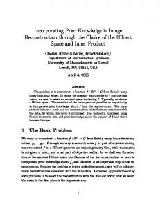
Example Let us consider the very common case in which the basis function G(x) is Gaussian. In this case its Fourier transform is also a Gaussian, and therefore G(s) = exp (?s2 ). The integral of eq. (9) can be performed

(Gradshtein and Ryzhik, 1981), to obtain the following form for H :

H (kxk; kxik) = e?(kxk2 +kxik2 )I 2d ?1 (2kxkkxik)

(10) where I d2 ?1 is the Bessel function of rst kind of imaginary argument (Gradshtein and Ryzhik, 1981, par. 8.406). A plot of this function in 2 dimensions is presented in gure (2), where we have set kxik = 2. It is clear that this function is a radial \bump" function, whose bump is concentrated on a circle of radius kxik. Any radial section of this function looks like a Gaussian function centered at kxik, providing a local, radially symmetric, form of approximation.

4.3 Radial Symmetry and \Virtual" Examples

In this section, we use the prior knowledge to generate new, \virtual" examples, from the existing data set. Let D = f(xi; yi ) 2 Rd  RgNi=1 be our data set, and let us assume that we know that the function h underlying the data has radial symmetry. This means that f (x) = f (R x) for all the possible rotation matrices R in d dimensions. Here  is a d ? 1 dimensional vector of parameters that represents a point of d?1 , the surface of the d-dimensional unit sphere. This property implies that if (xi; yi ) is an example of h, the points (R xi ; yi), for all  2 d?1 , are also examples of h, and we call these additional points the \virtual" examples. 15

circle of radius ||x||

H

y

x

Figure 2: The basis function H (kxk; kxik), for xi = (2; 0). Let us now consider a standard Radial Basis Functions approximation technique, of the form (3). Suppose for the moment that the function is invariant with respect to a nite number of rotations R1 ; : : :; Rn . Each example xi will therefore generate n virtual examples R1 xi ; : : :Rn xi , that can now be included in the expansion (3) together with the regular examples. It is trivial to see that, because of the invariance property of h, the coecients of the basis functions corresponding to the virtual examples will be equal to the coecients of the corresponding, original example. As a result we have that eq. (3) has to be replaced by

f (x) =

N X n X

ci G(x ? R xi) i=1 =0 0 = 0, so that R0 xi = xi.

where we have de ned We now relax the assumption that the function is invariant with respect to only a nite number of rotations, and allow  to span the entire surface d?1 . The equation above suggests to replace eq. (3) with the following:

f (x) =

N Z X i=1

ci

d?1

d d?1 () G(x ? R xi ) 16

(11)

where d d?1 () is the uniform measure over d?1 . Using the Hankel representation (7) for the radial function G in eq. (11), the integral over d?1 can be performed, and provides the result:

f (x) =

N X i=1

ci H (kxk; kxik)

where H (kxk; kxik) is given precisely be expression (9)! From this derivation it is clear that the basis function H (kxk; kxik) is an in nite superposition of Gaussian functions, whose centers uniformly cover the surface of the sphere of radius kxik. Therefore creating virtual examples seems to be, in a sense, the \right thing" to do, leading to the same result that one gets from the more \principled" and sophisticated approach of regularization theory. The appealing feature of the virtual examples technique is the fact that it can be applied in very general cases, in which it might be impossible to derive analytical results as the one derived in section 3.

5 Virtual Examples in Vision and Speech The goal of this paper is to suggest the creation of virtual examples as a technique to incorporate prior information in machine learning problems. The previous section shows how creating virtual examples can be equivalent to incorporation of the prior information as a regularizer within a framework for function learning. Thus the virtual example strategy can often be more than a good heuristic. We now turn our attention to some real world problems that arise in computer vision and speech recognition and give examples of how one might generate virtual examples under certain conditions. In the examples we are about to consider, the non-trivial part of the virtual example strategy is identifying the set of legal transformations that allow a new, valid, example to be created. In previous treatments of the machine learning problem that concentrated on function learning, the legal transformations were typically very simple and could easily be used to create examples. For example, whether the function is even or odd, or whether it has radial symmetry is easy to deal with. Imagine, instead, that one were interested in object recognition. How does one generate a new example? There are certain obvious cases. For example, by translating the image in the image plane or dilating the image (scale transformation) one could generate some trivial cases of new examples. However, there are some other 17

non obvious ones like rotation in depth, or changing the expression of a face that are signi cantly harder to realize. In the next section, we discuss the problem of object recognition, how to view it within a function learning paradigm, and how to generate non-trivial virtual examples for it.

5.1 Virtual Views for Object Recognition

Consider the problem of recognizing 3D objects from their 2D images. A particular class of 3D objects (like cars, or cubes, or faces) can be de ned in terms of pointwise features that have been put in correspondence with each other. If, for example, there are n features, and each feature is represented by its location in a 3D coordinate system (say by its x; y; z coordinates) then a particular view of a particular 3D object can be represented as a point in R3n: However, note that not all points in R3n correspond to valid views of 3D objects. Trying to learn this object class could be regarded as trying to learn a characteristic function in R3n ; i.e., a function of the form:

2 E  R3n 1E (x) : R3n ?! f0; 1g = 10 xotherwise When the 3D view is projected to 2D, then each 2D view can now be represented as a characteristic function over R2n : For problems such as these, one can rarely specify simple mathematical constraints (like radial symmetry etc.) on the characteristic functions. This makes the recognition problem particularly challenging. Consider, for example, the face recognition problem studied by Beymer (1994). The goal is to recognize faces of dierent people under a variety of views. One approach to this is to collect a large number of views from each person and train a classi er to recognize them. Shown in g. 3 are fteen views of one particular face that have been collected as training examples for that face. This relatively straightforward approach works but usually requires a large number of training examples. In contrast, an alternative strategy is to use some kind of prior knowledge about the class of faces in order to generate virtual examples or virtual \views". One could then train a view independent system on the basis of these virtual examples. This raises the question: if we are given examples of images belonging to some class, then can we generate new examples of images belonging to the same class? In order to do this we need to uncover the set of legal transformations that allow us to take elements of E and come up with other elements of E: Prior knowledge about the class of objects allow us to uncover such a set of valid transformation. 18

Figure 3: The pose-invariant, view-based face recognizer uses 15 views to model a person's face. From Beymer, 1994.

19

5.2 Symmetry as Prior Information

Poggio and Vetter (1992) examined in particular the case of bilateral symmetry of certain 3D objects, such as faces. Suppose that we have a model 2D view of an object and a pair of symmetric points in this 2D view. For our purposes, we can de ne an object to be bilaterally symmetric if the following transformation of any 2D view of a pair of symmetric points of the object yields a legal view of the pair, that is the orthographic projection of a rigid rotation of the object with

Dxpair = xpair

0 x1 1 xpair = BB@ xy2 CCA

0 ?x2 1 xpair = BB@ ?yx1 CCA

1

and

(12)

2

y2

y1

0 0 ?1 0 0 1 B ?1 0 0 0 CC D=B @ 0 0 0 1A:

0 0 1 0 Notice that symmetric pairs are the elementary features in this situations and points lying on the symmetry plane are degenerate cases of symmetric pairs. Geometrically, this simply means that for bilaterally symmetric objects simple transformations of a 2D view yield other views that are legal. The transformations are similar to mirroring one view around an axis in the image plane, as shown in Figure 4 top (where the left image is \mirrored" into the right one) and correspond { but only for a bilaterally symmetric object { to proper rotations of a rigid 3D object and their orthographic projection on the image plane. Using the transformation of equation 12 an additional view is generated from the one model view. If the two views are linearly independent, then one can resort to the 1.5 views theorem3 Using the notation introduced earlier, the set E de nes the space of valid image views of a particular object. The 1.5 views theorem states essentially that E can be regarded as a 6-dimensional vector space. Furthermore this basis can be computed from two linearly independent views. For further details on this, see Poggio and Vetter (1992). 3

20

Figure 4: Given a single 2D view (upper left), a new view (upper right) is generated under the assumption of bilateral symmetry. The two views are sucient to verify that a novel view (second row) corresponds to the same object as the rst. to compute a 3D basis that spans the space of the object. This allows us to compute a recognition function with just one true view. Bilateral symmetry has been used in face recognition systems (Beymer and Poggio, 1995) and psychophysical evidence supports its use by the human visual system (Schyns and Bultho, 1993; Troje and Bultho, 1995; Vetter, Poggio, and Bultho, 1994).

5.3 More General Transformations: Linear Object Classes

A more exible way to acquire information about how images of objects of a certain class change under pose, illumination and other transformations, is to learn the possible pattern of variabilities and class-speci c deformations from a representative training set of views of generic or prototypical objects of the same class { such as other faces. In particular, if the objects belong to a well behaved class known as a linear object class, the transformations can be easily learned. In this manner prior knowledge that the object class is linear can be utilized eectively to generate novel views that can be incorporated in the training process. Although this approach of linear classes originates from the proposal of Poggio and Vetter (1992) for countering the curse-of-dimensionality in applications of supervised learning techniques, more powerful versions have been developed recently. Techniques based on non-linear learning networks have been developed by Beymer, Shashua and Poggio (1993) as well as Beymer and Poggio (1995). For our purposes here, we now provide a brief 21

overview of the technique of linear classes for generating novel views of objects.

5.3.1 3D Objects, 2D Projections, and Linear Classes Consider a 3D view of a three-dimensional object that is de ned in terms of pointwise features (Poggio and Vetter, 1992). Such a 3D view can be represented by a vector X = (x1 ; y1; z1; x2; :::::; yn; zn )T , that is by the x; y; z coordinates of its n feature points. Further, assume that X 2