Compressed Sensing With Prior Information - CiteSeerX

IEEE TRANSACTIONS ON SIGNAL PROCESSING, VOL. 61, NO. 2, JANUARY 15, 2013

427

Compressed Sensing With Prior Information: Information-Theoretic Limits and Practical Decoders Jonathan Scarlett, Jamie S. Evans, Member, IEEE, and Subhrakanti Dey, Senior Member, IEEE

Abstract—This paper considers the problem of sparse signal recovery when the decoder has prior information on the sparsity pathas a rantern of the data. The data vector domly generated sparsity pattern, where the -th entry is non-zero with probability . Given knowledge of these probabilities, the random noisy projecdecoder attempts to recover based on tions. Information-theoretic limits on the number of measurements needed to recover the support set of perfectly are given, and it is shown that significantly fewer measurements can be used if the prior distribution is sufficiently non-uniform. Furthermore, extensions of Basis Pursuit, LASSO, and Orthogonal Matching Pursuit which exploit the prior information are presented. The improved performance of these methods over their standard counterparts is demonstrated using simulations. Index Terms—Basis pursuit, compressed sensing, compressive sampling, information-theoretic bounds, Lasso, orthogonal matching pursuit, prior information, sparsity pattern recovery, support recovery.

I. INTRODUCTION

T

HE problem of estimating an unknown vector from a number of noisy linear projections arises frequently in signal processing. Given a data vector and a known measurement matrix , the observation vector is of the form (1) where is additive noise. In the absence of any additional information on , this problem is well-posed only in the case that , where techniques such as least squares can be used. However, if is known to be sparse, i.e. where is the number of non-zero elements of , then an accurate estimate of can be obtained even with [1]. This phenomenon is known as compressed sensing or compressive sampling. A closely related problem is that of sparsity pattern recovery or support recovery, where the aim is to recover the support set of

Manuscript received August 25, 2011; revised January 27, 2012 and July 31, 2012; accepted September 22, 2012. Date of publication October 16, 2012; date of current version December 24, 2012. The associate editor coordinating the review of this manuscript and approving it for publication was Prof. Namrata Vaswani. J. Scarlett is with the Department of Engineering, University of Cambridge, Cambridge CB2 1PZ, U.K. (e-mail: [email protected]). J. S. Evans is with the Department of Electrical and Computer Systems Engineering, Monash University, Clayton, Victoria 3800, Australia (e-mail: jamie. [email protected]). S. Dey is with the Department of Electrical and Electronic Engineering, University of Melbourne, Parkville, Victoria 3052, Australia (e-mail: [email protected]). Color versions of one or more of the figures in this paper are available online at http://ieeexplore.ieee.org. Digital Object Identifier 10.1109/TSP.2012.2225051

, defined the be the positions of its non-zero entries. It is easy to see that if this problem is solved then the problem of sparse signal estimation is essentially solved as well, since one can then apply least squares restricted to the known support set. Recently there has been a great deal of work on the design and analysis of both tractable and intractable methods for compressed sensing and sparsity pattern recovery. The focus of this paper is on developing and analyzing methods which exploit prior information (other than being sparse). We are interested in information-theoretic limits on the performance of any decoder, as well as the design of tractable methods. These are complementary and both of great interest, with tractable methods being useful for practical systems, and information-theoretic limits being highly valuable for assessing the performance of tractable methods and determining the level of further improvement possible. The motivation for our work is the availability of prior information in several applications of compressed sensing. In sensor networks [2] the information obtained via a particular sensor could be used as information for another sensor. In functional medical resonance imaging [3], the prior information may arise from knowing which parts of the brain are usually associated with various decision making processes. In other applications, one may be interested in performing compressed sensing at multiple time instants, where the support set is correlated between times. This occurs, for example, in multipath channel estimation [4] and real time video reconstruction [5]. Finally, in some applications compressed sensing is one of several stages of an estimation problem, and additional information can be passed from an earlier stage [6]. The above applications involve many different types of prior information, making it difficult to obtain a tractable mathematical model which is suitable for each one. However, valuable insight can still be gained by analyzing specific models. In this paper, we assume prior information on the sparsity pattern of , but not the values of the non-zero entries. Specifically, we assume that the sparsity pattern is generated at random, with each entry of being non-zero with a given probability which is known at the decoder. A similar model is used in [7], and in [6] it is shown that such a model can provide insight into the compressed sensing problem even when prior information is not available. Specifically, [6] proposes a two-step recovery algorithm in which a hypothetical non-uniform sparsity model is generated in the first step, and a compressed sensing technique which exploits prior information is used in the second step. A. Notation We use the following notation throughout this paper. denotes the probability of an event, and denotes statistical expectation.

1053-587X/$31.00 © 2012 IEEE

means “distributed as”,

means “approximately

428


distributed as”, and means “proportional to” in a probabilistic sense. The Gaussian distribution is denoted by . The support of a vector is denoted by . All logarithms have base , and is the binary entropy function in nats. denotes magnitude when applied to a number, and denotes cardinality when applied to a finite set. denotes the -norm of a vector if , and the number of non-zero elements in a vector (commonly referred to as the -norm) if . For an index set and matrix , denotes the submatrix of containing the columns indexed by . Similarly, for a vector , denotes the subvector of containing the elements indexed by . The transpose of a vector or matrix is denoted by . For two functions and , we write if for some constant when is sufficiently large, if , if , if , and if both and hold.

TABLE I SUMMARY OF DEFINITIONS

B. Problem Statement The data vector and measurement vector are related by and has en(1). We assume that has entries for and .1 tries The -th column of is denoted by . The data vector is generated as follows. The -th entry of is given by (2) is a deterministic non-zero value, and where is a random variable indicating whether the entry is non-zero. The probability of being equal to one is denoted by , and we assume that the random variables are independent. The support set of is therefore distributed according to (3) The task of the decoder is to estimate from the observation vector given in (1), using as prior information. We refer to as the support probability of the -th entry of . We model the support probabilities as follows. For a proportion of the coefficients have support and for probability equal to , where all . That is, the coefficients are divided into groups, where the support probabilities of all coefficients in a given group are equal. The number of coefficients in group is denoted by . We define the average binary entropy of the support probabilities as (4) where entropy function.

is the binary

1Some authors use different normalizations, such as each entry of and having variance and respectively. This does not affect the results provided the SNR is the same.

For a given support set , we denote the number of non-zero entries by . The average of with respect to the distribution in (3) is denoted by , i.e. (5) For a given data vector , the smallest and largest magnitudes are denoted by and respectively. The smallest and largest magnitudes of are denoted by and respectively. For reference, the definitions of the main symbols used throughout the paper are summarized in Table I. C. Contributions and Previous Work 1) Overview of Standard Techniques: Before summarizing our contributions, we outline the practical methods for compressed sensing without prior information (other than being sparse) most relevant to this paper. Two commonly used -based methods are Basis Pursuit (BP) [8] and Least Absolute Shrinkage and Selection Operator (LASSO) [9], which are respectively described by (6) (7) where is a parameter to LASSO which controls the tradeoff between sparsity and goodness of fit. These techniques are closely related, with BP being the convex relaxation of the intractable minimization problem , and LASSO being the convex relaxation of least squares with an penalty. Both have been shown to give good performance in practical systems, with the required number of measurements generally ranging from to

SCARLETT et al.: COMPRESSED SENSING WITH PRIOR INFORMATION

depending on the performance requirements; see [8], [10] for details. Orthogonal Matching Pursuit (OMP) uses a greedy approach rather than optimization of an objective [11]. We outline the algorithm here and refer the reader to [11] for details. The decoder repeatedly adds to the support estimate the coefficient whose column of is most highly correlated with a residual vector . The first residual vector used is , and subsequent residuals are computed as where is the least squares estimate of restricted to the support set obtained so far. The algorithm terminates when the number of iterations exceeds a threshold, or when the norm of the residual falls below a threshold. This technique is computationally efficient and has been shown to exhibit performance which is comparable to BP and LASSO [12]. 2) Contributions: A summary of our contributions is as follows: • We extend the techniques of [13] to obtain both sufficient and necessary conditions on the number of measurements required for exact recovery of the support set as and grow large, with known at the decoder. Sufficient conditions are obtained via the analysis of a joint typicality decoder, and necessary conditions are obtained by an analogy to a multiple input single output (MISO) communication channel in which the decoder attempts to recover the support set. We show that the introduction of prior information can significantly reduce the number of measurements required. In particular, it is shown that measurements suffice under various assumptions. • We present three practical decoding techniques for compressed sensing with prior information, which are extensions of BP, LASSO and OMP. The idea is to introduce weights which depend on the support probabilities, so that coefficients with higher probability are favored. For the extensions of BP and LASSO, the term in the objective is replaced by , and we motivate the use of the weights . For the extension of OMP the decoder greedily makes a decision based on the sum of a correlation term and a weighting term, rather than just the correlation term. We motivate the use of weights proportional to . • Using simulations, we demonstrate the improved performance of our practical decoding techniques compared to their standard counterparts. It is seen empirically that has a significant effect on performance when using these techniques. Furthermore, we explore the impact on performance of noise and mismatch. 3) Previous Work on Information-Theoretic Limits: Previous work on information-theoretic limits on exact sparsity pattern recovery is as follows. In [14], necessary conditions for the maximum likelihood (ML) decoder are obtained, and a simple maximum correlation decoder is analyzed. In [15] an analogy is drawn between sparsity pattern recovery and the Gaussian multiple access channel in order to find both necessary and sufficient conditions on . In [16], sufficient conditions are obtained for the ML decoder, and necessary conditions are found based on Fano’s inequality. These necessary conditions are tightened in [17], and a comparison between dense and sparse ensembles is performed. In [18], sufficient conditions are derived and shown to be tight in a scaling-law sense by comparison to the necessary

429

conditions of [17]. For information-theoretic limits with respect to other performance metrics, see [13], [19], [20]. In contrast to our work, these papers consider the case that all support sets of a given cardinality are equiprobable. 4) Previous Work on Exploiting Prior Information: In [21] a method called Modified-CS is proposed, in which the objective function only penalizes coefficients outside a partially known support. In [7] a Grassman angle approach is used to provide a comprehensive analysis of a weighted minimization problem, focusing primarily on the case that there are only two different probabilities, and hence only two weights. The authors provide a method for optimizing the weights with respect to various metrics, but due to the highly non-convex nature of the problem, significant computation is needed. The introduction of weights into LASSO and OMP is proposed in [22] for the dual problem of sparse signal approximation with prior information. We present a comparison of our techniques to those of [7], [21], [22] in Section IV-D. In [23] the method of model-based compressed sensing is introduced, in which the support is known to have a particular structure. Specifically, only a subset of the supports of a given cardinality can occur. Among others, this includes block sparsity [24] and tree sparsity [25] as special cases; see [23] for a complete set of references. While the framework of [23] does not include our setup as a special case, we draw some connections between the two in Section II-C-4. In [26], a Kalman filter is used to exploit correlations between the values of under the assumption that the support changes very slowly. In [27], a Bayesian learning approach is used to account for correlations in the measurement vectors, but again the focus is on correlations between the values of , rather than the support. D. Paper Organization In Section II we present a summary and discussion of our information-theoretic results, which are given in Theorems 1 and 2. In Section III we give proofs of these theorems. In Section IV we present our practical decoding techniques and compare them to existing methods, as well as analyzing their performance via simulations. Conclusions are drawn in Section V. II. INFORMATION-THEORETIC RESULTS Before stating the main theorems, we give a precise definition of the performance metric. For each , let the number of groups and the corresponding and be given, along . The support set is generated according with the gains to (3), yielding the data vector . The measurement matrix and noise vector are generated at random, yielding the observation vector . The decoder takes as input and forms an estimate of the support set ; the quantities , , , and are assumed to be known. An error is said to have occurred if . For a given support set , we define the error probability (8) where the probability is taken with respect to statistics of . Similarly, we define

and (9)

430


where the probability is taken with respect to statistics of , and . That is, the quantity in (9) is obtained by averaging (8) over the distribution of in (3). The value in (4) represents the average uncertainty of whether the coefficients are going to be non-zero or not. It plays a major role in both the necessary and sufficient conditions of the number of measurements, as we will see in Section II-B. We remark that while can be independent of in the linear regime , it tends to zero for large in the sublinear regime , so the presence of the term in the number of measurements does not imply that the overall value is . Throughout this section, we will sometimes use a superscript to make the dependence of a variable on explicit (e.g. ). The superscript will be omitted when no confusion arises from doing so. A. Typicality We begin by introducing the notion of typicality with respect to the support probabilities . We define to be the number of non-zero coefficients in the set from group . Definition 1: (Typicality) A support set is -typical if

literature, we do not assume that the decoder has knowledge of . Theorem 1: (Sufficient Conditions) Fix , and , and let is bounded away from 1, and

be such that

. Let trary sequence of support sets satisfying

be an arbi. If

, then there exists a decoder such that the error probability provided that

tends to zero as

,

(14) . for some Proof: See Section III-A. Theorem 2: (Necessary Conditions) Fix and let that

,

and

, be such

. Let

be an arbitrary sequence of support , and let be the corresets satisfying sponding data vector. Then the error probability for any decoder is bounded away from zero as if

(10) for all . The set of all -typical supports is denoted by . The following proposition gives useful properties of the typical set. Proposition 1: (i) For any , the cardinality of satisfies (11) (ii) The cardinality of the typical set satisfies (12) (iii) If

and , then

(15)

for some

. Consequently, if

and then measurements are necessary. Proof: See Section III-B. Theorems 1 and 2 give conditions on such that for a given sequence of typical support sets . We can obtain conditions on such that by writing (16)

for all

(17) (13) Proof: These follow using standard proofs based on the method of types, e.g. see [28]. For property (iii), the condition implies that the law of large numbers holds for each group, and thus (13) follows from the condition . B. Statement of Main Results Here we present two theorems summarizing the asymptotic bounds on the number of measurements needed under various assumptions. It should be noted that the sufficient conditions are based on a joint typicality decoder which is too complex to be used in practice, whereas the necessary conditions bound the performance of any decoder. In contrast to most of the existing

(18) where (18) follows from (13). Corollary 1: Let the assumptions of Theorem 1 be satisfied. If

, then there exists a decoder such that the

error probability

tends to zero as

, provided that (19)

for some . Proof: We obtain (19) by combining (14) and (18), and noting that and can be chosen to be arbitrarily small. The


431

condition in Theorem 1 is satisfied for all since by definition. Corollary 2: Let the assumptions of Theorem 2 be satisfied. for any decoder is bounded away The error probability from zero as if

(20) for some . Proof: For any

, we have (21) (22)

where we have used (11) and the definition of . It follows that the necessary number of measurements in (15) can be weakened to (23) where . The corollary follows by combining (18) and (23) and noting that , and therefore , can be chosen to be arbitrarily small. C. Discussion Since Theorems 1 and 2 apply for any , it follows from (11) that the corresponding are close to , and the resulting necessary and sufficient conditions are unchanged in a scaling-law sense when is replaced by . For the remainder of the section, we express the results in terms of . Theorem 1 implies that measurements are sufficient. Theorem 2 states that under the same conditions as Theorem 1, measurements are necessary, meaning that there is a gap between the scaling of the necessary and sufficient conditions. Nevertheless, these bounds still provide valuable insight into the number of measurements needed with prior information. In particular, we show in Section II-C-3 that the sufficient number of measurements with prior information can have a lower rate of growth than the necessary number of measurements in the absence of prior information. In the case that , our sufficient and necessary conditions match those of [13]. This is unsurprising, since our proofs are based on techniques used in [13]. 1) Discussion of Assumptions: We make the following remarks on the assumptions of Theorems 1 and 2. • The condition that in Theorem 1 is a generalization of the assumptions in [13] that in the linear regime , and in the sublinear regime . The reason such restrictions on are required is that due to the presence of noise, perfect recovery of the sup-

port is not possible when the coefficients can be arbitrarily small. • The conditions that remains bounded away from 1 and are mainly for technical reasons. The first is very mild, since would mean that nearly all coefficients of are non-zero with high probability. The condition that states that number of groups does not grow unbounded, hence limiting the growth rate of certain expressions in the analysis. • The condition states that each group has an unbounded average number of both zero and non-zero coefficients. This is for technical reasons relating to typicality (see Definition 1). Defining , we see that is of limited interest, since it implies that asymptotically either all or none of the coefficients of the group are zero with probability approaching one. However, could be of interest. For example, a group with a large number of low probability coefficients leading to a Poisson distribution would give . In this paper, we assume there are no such groups. 2) Discussion of Linear Regime: A suitable model for the linear regime is one in which the number of groups and their associated probabilities are independent of . In this case is constant and hence the necessary and sufficient number of measurements is under the assumptions of Theorem 1, thus matching the case that the prior information is absent [13]. However, prior information can decrease the constant factor in the sufficient number of measurements. In particular, a simple application of Jensen’s inequality in (4) yields , where the right-hand side recovers the case with no prior information. 3) Discussion of Sublinear Regime: For the sublinear regime, a comparison of our results to those without prior information is presented in Table II under various scalings of , where it is assumed that . We see that depending on the scaling of , our sufficient conditions can exhibit better scaling than the necessary and sufficient conditions without prior information. For example, consider the case and , so that coefficients are in that group 1 and for some that

are in group 2. We let . Using , it follows , and hence (24) (25)

where (25) follows by noting that the term dominates in the sublinear regime and has the same rate of growth as . Supposing now that , we see that measurements are sufficient. From Table II, the necessary number of measurements without prior information is and for the cases and respectively. We therefore achieve improved , and in scaling in the former case for any the latter case for any

.

432


TABLE II NECESSARY AND SUFFICIENT NUMBER OF MEASUREMENTS IN THE SUBLINEAR REGIME WITH AND WITHOUT PRIOR INFORMATION

Connections With Model-Based CS: In [23] it is assumed that the data vector’s support belongs to some set containing supports of cardinality . It is shown that with measurements, an error of is possible, where is the decoder output and and are constants. It is interesting to note that the scaling matches the scaling given in Theorem 1 when we substitute . However, Theorem 1 does not follow from this result, since the performance metrics differ and our setup allows for to vary with different realizations of . III. PROOFS OF INFORMATION-THEORETIC RESULTS The proof of Theorem 1, given in Section III-A, uses a joint typicality decoder which is suboptimal but simpler to analyze than the optimal decoder. The proof of Theorem 2, given in Section III-B, uses an analogy to a MISO communication channel. Before presenting the proofs, we give bounds on the term , which appears in the upper bound on the typical set size in (12). Proposition 2: . (i) If is bounded away from 1 then and for all (ii) If , then . Proof: For the first part, we apply Jensen’s inequality to obtain (26) It is straightforward to show that this behaves as by treating the linear and sublinear regimes separately and using the condition that is bounded away from 1 in the linear regime. For the second part, we write and focus on the group with the largest . Since there are only groups and coefficients in total, there must be at least one group with coefficients. Assuming without loss of generality that group 1 has the largest number of coefficients, we write (27) (28) , and we have included in the numerwhere ators and denominators inside the logarithms for convenience. We show that this grows faster than by treating the cases and separately. Starting with the former, the right hand side of (27) is lower bounded by . If we obtain

since

. If

in the case that argument holds using and

, which grows faster than we obtain . Hence . When , a similar and , and treating the cases separately.

A. Proof of Theorem 1 Along with Definition 1, we will make use of the following definition of joint typicality from [13]. Definition 2: [13] (Joint Typicality) The observation vector and a set of indices are -jointly typical if and (29) is an orthogonal projecwhere tion matrix. The set of all sequences which are -jointly typical with is denoted by . Using the notions of typicality in Definitions 1 and 2, the decoder estimates to be a support set in the intersection of and . If no such support exists, an error is declared. If multiple such supports exist, the decoder chooses the one with the smallest cardinality, with ties broken arbitrarily. We define the following events: • : The true support is not jointly typical with •

: Another typical support is jointly typical with and has a cardinality which does not exceed the true support ( for some , ) The overall error probability is then bounded as (30) To perform the analysis, we make use of the following lemma from [13]. We note that the bounds given in the lemma hold for the given support set , with the associated probabilities denoted by . Lemma 1: [13] If is the true support set and is another support set, then (31)

(32)


where and . In particular, the following corollary will be useful. for some Corollary 3: [13] Choosing the bounds in Lemma 1 imply

433

where , (42)

(33)

Again bounding

using (11), it follows that (43)

(34)

(44)

where . Since we are focusing on the case that and are both elements of , we can further bound (33), (34) using the cardinality bound in (11), yielding

Thus, a sufficient condition for to decay to zero is that tends to for all . We show that this condition is satisfied by treating the cases and separately. Starting with the former, we have

(35) (45) (36) . Using the bound on in We begin by bounding (14) and the assumption that , we have . Since grows faster than by assumption, it follows that . Substituting this into (35), it follows that decays to zero for large . The remainder of the proof shows that also decays to zero for large , and thus the overall error probability tends to zero. We define as the number of supports with , and . , and hence (12) A trivial upper bound gives yields (37) Furthermore, a simple counting argument gives (38) which, using

, implies that (39)

requires Since the event attention to the case that . Hence, from (39), we obtain

, we can limit to our , or equivalently

(40) where we have bounded using (11). Combining (37) and (40) with (36) and applying the union bound, we obtain (41)

(46) (47) (48) , (46) follows from the , and (47) follows from , the assumption of the theorem that grows faster than , and the assumption that . , the term asympIn the case that totically tends to 1, and we have where (45) follows from bound on in (14) and since

(49) where we have used . By rearranging, it is straightforward to show that this expression tends to for any that satisfies (14) with . B. Proof of Theorem 2 Throughout the proof, we will make use of the fact that the support set cardinalities must satisfy (11), since by assumption. We first prove the lower bound of . With non-zero coefficients and groups, there must exist a group with at least non-zero coefficients. Without loss of generality, we assume group 1 is such a group. Suppose that all other groups’ coefficients, as well as the realization of the additive noise , are revealed to the decoder. The decoder is left with the task of identifying which of the coefficients of group 1 are non-zero. The problem is therefore reduced to finding a sparsity pattern of coefficients for a vector of dimension in the absence of noise, and with no prior

434


information. This requires measurements [14], and is neceshence using (11) we obtain that sary. To prove the other term in the lower bound in (15), we consider a MISO channel which emulates support recovery with additional information at the decoder. We note that this proof is a more straightforward extension of [13] than that of the sufficient conditions, but we describe the setup for completeness. We assume that the decoder has access not only to the probability vector , but also to the support set size and the coefficients corresponding to the true support . Clearly the error probability in this scenario is no higher than that of the original sparsity pattern recovery problem. The encoder maps the support to the codeword which is transmitted over a -input MISO channel in uses. The channel is specified by , so that the received signal is . Based on , the decoder constructs the support estimate . For a given , the sum capacity of the channel is given2 by [13]

From (10),

differs from

sumption that , it follows that differs from by no more than ; this can be seen graphically by noting that the difference is maximized at the endpoints. Continuing, and also applying , we obtain (56) Finally, applying yields

(see Proposition 2) and (57)

Applying Proposition 3 to (51), the main part of the theorem is proved. To prove the second part of the theorem, we show that and imply

. It follows from ,

and that , so it remains to show that

(50) are obtained by comparing (50) to Necessary conditions on the amount of information which must be transmitted over the channel. Specifically, if nats must be transmitted over the channel, then a necessary condition on is

by no more than . From the as-

. We rewrite , and substitute

The following proposition shows that the number of nats required is essentially . Proposition 3: For sufficiently large , the number of nats required to identify the support set with vanishing probability of error satisfies (52)

from , or equivalently

Proposition 2 to obtain . Since follows that

(51)

as

, it .

IV. PRACTICAL DECODING TECHNIQUES Motivated by practical systems, we present extensions to three common techniques for sparse signal recovery, namely Basis Pursuit, LASSO and Orthogonal Matching Pursuit. In order to exploit the prior information, we introduce weights dependent on the support probabilities into each of these techniques, so that the decoder is more inclined to declare a coefficient to be non-zero when it has a higher probability. A. Extensions of BP and LASSO

for any . Proof: We let denote the number of non-zero coefficients in the set from group . We lower bound by counting the number of supports for which for all . Writing as a shorthand for , we have

Our extensions of BP and LASSO are respectively given by

(53)

We call these Log-Weighted Basis Pursuit (LW-BP) and LogWeighted LASSO (LW-LASSO) respectively. As is the case in LASSO, is a parameter which controls the tradeoff between sparsity and goodness of fit. It is well known that BP is the convex relaxation of minimization in the absence of noise [8]. We similarly motivate LW-BP as the convex relaxation of a problem which maximizes a combination of sparsity and probability in the absence of noise. From (3), the most probable signal consistent with is given by

(54) where (54) follows from the logarithm of (54) gives

. Taking

(55) 2Compared to [13], an extra factor of 1/2 appears in our expression because we are considering the real case.

(58) (59)

(60)


435

since maximizing a probability is equivalent to maximizing its logarithm. The objective in (60) contains two summations; the first favors the inclusion of higher probability coefficients in the support, while the second favors the exclusion of lower probability coefficients. For the purposes of promoting sparsity, and also to allow a convex relaxation of the problem, we consider the problem containing only the former summation, given by (61) For example, in the case that each is equal, the objective in (61) is proportional to . Relaxing to the concave function , we obtain LW-BP in (58). The weights of have the desirable properties of being continuous and decreasing, with an infinite penalty when the probability is zero and no penalty when the probability is 1. Using a similar argument, LW-LASSO can be motivated by starting with the problem of maximizing when the noise term contains independent Gaussian entries with variance . In this case, using the definition of the Gaussian probability density function, we have (62) and hence maximizing is equivalent to minimizing . Assuming that the only knowledge of is the support probabilities, a similar argument to the one above gives the equation for LW-LASSO in (59).

factor

increases with

explained by the fact that if the measurements are more noisy then they are less reliable, so the prior information is relied on more. A similar argument applies for the dependence on . Finally, the term merely scales the weights to match the amplitude of the non-zero coefficients, making the decision unchanged if, for example, and are both scaled by the same amount. The expression in (63) motivates the use of the a weight function which varies with the iteration number, with (63) being used on the first iteration, but then substituting (64) on the -th iteration. In the case that is not known, one could replace the right-hand side of (64) with and terminate the algorithm when the norm of the residual falls below a threshold. For simplicity, we focus on the case that is known. In the case that the non-zero coefficients do not have equal amplitude but are instead independently drawn according to some distribution , we can replace each occurrence of in (63) with a suitable average , such as or . While this is not necessarily optimal, it keeps the algorithm simple while still effectively exploiting the prior information, as we will see via simulations in the following subsection. An alternative approach would be to take the constant factors as design parameters. The steps of LW-OMP are summarized in Algorithm 1. Algorithm 1: Logit Weighted Orthogonal Matching Pursuit

B. Extension of Orthogonal Matching Pursuit

Inputs:

The idea of OMP is to repeatedly add the index which has the highest correlation with a residual vector . We introduce an algorithm which we call Logit-Weighted Orthogonal Matching Pursuit (LW-OMP), in which instead the highest is added at each step, where is proportional to the logit function . More precisely, in Appendix A we show that among all additive weight functions,3 the choice

Outputs: Support set estimate estimate

(63) approximately minimizes the probability of incorrectly choosing a zero coefficient over a non-zero coefficient in the case that is the random noisy projection of a data vector containing non-zero coefficients of equal amplitude , and each term of the additive noise has variance .4 We briefly discuss the resulting terms in the expression. The only part containing is , which has the desirable properties of being continuous and increasing, with an infinite penalty when is zero and an infinite reward when is 1. The constant 3A justification for the use of an additive (rather than multiplicative) weight function is given in Section IV-D. 4The resulting equations will vary when different normalizations are used for the measurement matrix and noise vector, but these can be incorporated into the values of and .

, which can be

, , ,

,

Algorithm: 1) Initialize the residual vector , and set 2) While :

, data vector

and support estimate

a) Set b) Set maximum is over c) Set and is the empty matrix d) Set e) Increment 3) Return and

, where the , where and

C. Simulations In this section we simulate LW-BP, LW-LASSO and LW-OMP for various and with , , and runs per simulation. The non-zero gains are randomly drawn according to N(0,1). We set and choose the such that for all . That is, each group has an average of four non-zero coefficients. We simulate four

436


TABLE III GROUP SIZES USED IN THE SIMULATIONS

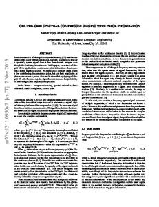
different group arrangements each with different values of , as given in Table III. We measure the performance of each technique by comparing coeffithe true support to , defined to contain the cients of with the largest magnitude, where is the estimate of . The performance metric we study is the average proportion of coefficients recovered, given by (65)

noisier setting of the dependence is somewhat weaker. For LW-OMP, the dependence is weaker at both values of . Lastly, we examine the effect of mismatch on each technique. We focus on Simulation 3 with and assume that the true value of is used in each method, but is replaced by . For example, in LW-BP the weights of are replaced by for . Fig. 2 plots the performance of each technique as a function of . The left-most points correspond to and therefore give the performance when the prior information is ignored altogether. We see that even with mismatch the performance is improved for the entire range plotted. Furthermore, the performance of each technique remains close to its peak for a wide range of , suggesting a good robustness against mismatch. The peak in each plot is not at , suggesting that weights are slightly is close to suboptimal. However, the performance at the peak for all three techniques, particularly for LW-BP and LW-LASSO. D. Comparisons to Existing Work

where is the number of runs per simulation, is the true support on the -th run and is the support estimate on the -th run. Fig. 1(a) shows the average proportion of coefficients recovered using LW-BP for both and . Fig. 1(c) shows the performance of LW-LASSO with where is the average weight. Fig. 1(e) shows the performance of LW-OMP using , which is the average magnitude of an N(0,1) random variable. Simulation 1 represents the case where there is no prior information, since in this case all support probabilities are equal and the techniques reduce to the standard versions on which they were based; the corresponding curves are shown in bold. For all three techniques, the weighted versions result in better performance, particularly when the prior distribution is far from uniform. Furthermore, the improvement is evident using both and . Comparing the three methods, we see that LW-LASSO tends to give the best performance. In comparison, the performance of LW-BP is nearly identical with but slightly worse with . The performance of LW-OMP is similar to LW-LASSO for high values of , but worse at low values of . The information-theoretic results of Section II give sufficient and necessary conditions on for perfect support recovery which are affine in . We now investigate whether a similar dependence on exists for these practical decoding techniques under less strict performance requirements. If the proportion of coefficients recovered for given values of and depends inversely on an affine function of , then we expect the plots of vs. to be the same for each of the four group arrangements, for some constant . Figs. 1(b) and 1(d) plot this relationship for LW-BP and LW-LASSO respectively, both with . Fig. 1(f) shows the relationship for LW-OMP with . The plots align very closely for LW-BP and LW-LASSO in the case that , indicating that does have a significant effect on performance. Specifically, this suggests that for given values of and , the minimum number of measurements required to recover a certain proportion of the coefficients is approximately proportional to . In the

The Modified-CS technique [21] performs a similar minimization to BP, but with zero penalty on coefficients within a partially known support. This can be viewed as an extreme case of LW-BP, where for coefficients in the partially known support, and all other are equal to some constant in the range (0,1). In [7], a similar minimization technique to LW-BP is presented, with the main focus being on the case that there are only two different probabilities and hence two weights. A method is given for optimizing the weights, but it involves searching the space of potential weights and performing a significant amount of computation to decide which to use. This makes LW-BP more suitable when there are a wide range of different probabilities, or in the case that the probabilities are varying with time and a such a search is not feasible (e.g. in online applications). An iterative reweighted minimization technique is proposed in [29], in which the estimate of on the -th iteration is given by (66)

. The weights are inifor some non-negative weights and then reweighted as , tialized as is the -th entry of and is a positive constant. where While (66) bears a strong resemblance to LW-BP, the reason for introducing the weights is different. Instead of exploiting information which is known a priori, the weights in (66) serve to reduce the dependence of the objective on the magnitudes of , hence making the optimization more similar to that of minimization [29]. In [22], a similar technique to LW-LASSO appears under the name Weighted Basis Pursuit Denoising (W-BPDN). Specifically, the objective function is where is some measure of the a priori likelihood of each term being non-zero, but not necessarily a probability measure. Its use generally relies on already knowing a good choice of weights, or being able to tune them via a parameter search. On the other hand, in LW-LASSO the weights are a simple function


437

Fig. 1. Algorithm performance without prior information (simulation 1) and with prior information (simulations 2–4). (a) LW-BP; (b) LW-BP (scaled); (c) LW-LASSO; (d) LW-LASSO (scaled); (e) LW-OMP; (f) LW-OMP (scaled). The legends for (a), (c) and (e) are shown in (b), (d) and (f) respectively.

of the support probabilities, making it more suitable for applications where the prior information arises in this form. Similarly, a technique called Weighted Matching Pursuit (W-MP) appears in [22]. As discussed in [22], can be viewed as a measure of when

and

is Gaussian. The authors in [22] state that since , prior information can be incorporated by instead adding the highest for some weight . However, we argue that since actually arises as a term in the logarithm of , additive weights are more

438


of 1. Hence by the central limit theorem, Similarly, for any ,

.

. Therefore (68)

Consider

and , and let and is incorrectly favored over index when . We denote the probability of this event . Using the expression in (68), we obtain

. Index by

(69) where is the probability that an N(0,1) random variable exceeds . Similarly, we define as the probability of being incorrectly favored over conditioned on and . Our aim is to minimize the probability of exactly one of the two indices being non-zero but the other one being preferred, given by

Fig. 2. Proportion of coefficients recovered using a mismatched value of in Simulation 3 with and . The case indicates performance without prior information.

(70) suitable than multiplicative weights. Furthermore, similarly to LW-LASSO, an advantage of LW-OMP is that the weights are a simple function of the corresponding support probabilities. (71) V. CONCLUSION We have studied the problem of sparse signal recovery with prior information on the sparsity pattern of the data. We have presented information-theoretic limits on the number of measurements required, with the main result being that measurements are sufficient under various assumptions. In many cases, this is a significant improvement over the number of measurements required without prior information. Extensions of BP, LASSO and OMP have been given, each of which uses weights in order to exploit the prior information. The proposed weights are simple functions of the corresponding support probabilities, making the techniques practical and easy to implement, while still giving good improvements in performance compared to their standard counterparts. APPENDIX

. Setting the partial derivative with respect where to to zero and simplifying, we obtain (72) Setting to 0 yields

and taking the limit as

and

tend

(73) The derivation is concluded by integrating both sides of (73). REFERENCES

A. Derivation of LW-OMP Weights We consider the simple case in which there are non-zero coefficients in , each having a fixed value . Without loss of generality it can be assumed that , and thus the measurement vector is given by (67) by the law of large Assuming is sufficiently large, numbers. For , where and are independent random variables with a mean 0 and a variance of 1, meaning their product also has a mean of 0 and a variance

[1] E. J. Candès and M. B. Waki, “An introduction to compressive sampling,” IEEE Signal Process. Mag., vol. 25, no. 2, pp. 21–30, Mar. 2008. [2] W. Bajwa, J. Haupt, A. Sayeed, and R. Nowak, “Compressive wireless sensing,” presented at the Int. Conf. Inf. Process. Sensor Netw., Nashville, TN, Apr. 2006. [3] K. Lee, S. Tak, and J. C. Ye, “A data-driven sparse GLM for fMRI analysis using sparse dictionary learning with MDL criterion,” IEEE Trans. Med. Imag., vol. 30, no. 5, pp. 1076–1089, May 2011. [4] W. U. Bajwa, J. Haupt, A. M. Sayeed, and R. Nowak, “Compressed channel sensing: A new approach to estimating sparse multipath channels,” Proc. IEEE, vol. 98, no. 6, pp. 1058–1076, Jun. 2010. [5] M. B. Wakin, J. N. Laska, M. F. Duarte, D. Baron, S. Sarvotham, D. Takhar, K. F. Kelly, and R. G. Baraniu, “An architecture for compressive imaging,” presented at the IEEE Int. Conf. Image Process., Atlanta, GA, Oct. 2006. [6] M. A. Khajehnejad, W. Xu, A. S. Avestimehr, and B. Hassibi, “Imminiproved sparse recovery thresholds with two-step reweighted mization,” presented at the IEEE Int. Symp. Inf. Theory, Pasadena, CA, Jun. 2010.


[7] M. A. Khajehnejad, W. Xu, A. S. Avestimehr, and B. Hassibi, “Anminimization for sparse recovery with nonunialyzing weighted form sparse models,” IEEE Trans. Signal Process., vol. 59, no. 5, pp. 1985–2001, May 2011. [8] E. J. Candès and T. Tao, “Decoding by linear programming,” IEEE Trans. Inf. Theory, vol. 51, no. 12, pp. 4203–4215, Dec. 2005. [9] R. Tibshirani, “Regression shrinkage and selection via the lasso,” J. Roy. Statist. Soc., vol. 58, no. 1, pp. 267–288, 1996. [10] M. J. Wainwright, “Sharp thresholds for high-dimensional and noisy sparsity recovery using -constrained quadratic programming (Lasso),” IEEE Trans. Inf. Theory, vol. 55, no. 5, pp. 2183–2202, May 2009. [11] Y. C. Pati, R. Rezaiifaarn, and P. Krishnaprasad, “Orthogonal matching pursuit: Recursive function approximation with applications to wavelet decomposition,” presented at the Annu. Asilomar Conf., Pacific Grove, CA, Nov. 1993. [12] J. A. Tropp and A. C. Gilbert, “Signal recovery from random measurements via orthogonal matching pursuit,” IEEE Trans. Inf. Theory, vol. 53, no. 12, pp. 4655–4666, Dec. 2007. [13] M. Akcakaya and V. Tarokh, “Shannon-theoretic limits on noisy compressive sampling,” IEEE Trans. Inf. Theory, vol. 56, no. 1, pp. 492–504, Jan. 2010. [14] A. K. Fletcher, S. Rangan, and V. K. Goyal, “Necessary and sufficient conditions for sparsity pattern recovery,” IEEE Trans. Inf. Theory, vol. 55, no. 12, pp. 5758–5772, Dec. 2009. [15] Y. Jin, Y. Kim, and B. D. Rao, “Support recovery of sparse signals via multiple-access communication techniques,” IEEE Trans. Inf. Theory, vol. 57, no. 12, pp. 7877–7892, Dec. 2011. [16] M. J. Wainwright, “Information-theoretic limits on sparsity recovery in the high-dimensional and noisy setting,” IEEE Trans. Inf. Theory, vol. 55, no. 12, pp. 5728–5741, Dec. 2009. [17] W. Wang, M. J. Wainwright, and K. Ramchandran, “Information-theoretic limits on sparse signal recovery: Dense versus sparse measurement matrices,” IEEE Trans. Inf. Theory, vol. 56, no. 6, pp. 2967–2979, Jun. 2010. [18] K. R. Rad, “Nearly sharp sufficient conditions on exact sparsity pattern recovery,” IEEE Trans. Inf. Theory, vol. 57, pp. 4672–4679, July 2011. [19] G. Reeves and M. Gastpar, “Approximate sparsity pattern recovery: Information-theoretic lower bounds,” [Online]. Available: http://arxiv. org/abs/1002.4458, arXiv:1002.4458v2 [cs.IT]. [20] S. Aeron, V. Saligrama, and M. Zhao, “Information theoretic bounds for compressed sensing,” IEEE Trans. Inf. Theory, vol. 56, no. 10, pp. 5111–5130, Oct. 2010. [21] N. Vaswani and W. Lu, “Modified-CS: Modifying compressive sensing for problems with partially known support,” IEEE Trans. Signal Process., vol. 58, no. 9, pp. 4595–4607, Sep. 2010. [22] Ò. D. Escoda, L. Granai, and P. Vandergheynst, “On the use of a priori information for sparse signal approximations,” IEEE Trans. Signal Process., vol. 54, no. 9, pp. 3468–3482, Sep. 2006. [23] R. G. Baraniuk, V. Cevher, M. F. Duarte, and C. Hegde, “Model-based compressive sensing,” IEEE Trans. Inf. Theory, vol. 56, no. 4, pp. 1982–2001, Apr. 2010. [24] M. Stojnic, F. Parvaresh, and B. Hassibi, “On the reconstruction of block-sparse signals with an optimal number of measurements,” IEEE Trans. Signal Process., vol. 57, no. 8, pp. 3075–3085, Aug. 2009. [25] R. Baraniuk, “Optimal tree approximation with wavelets,” in Proc. SPIE Wavelet App. Signal Image Process., Denver, CO, Jul. 1999, vol. 3813, pp. 196–207. [26] N. Vaswani, “Kalman filtered compressed sensing,” presented at the IEEE Int. Conf. Image Process., San Diego, CA, Oct. 2008. [27] Z. Zhang and B. Rao, “Sparse signal recovery with temporally correlated source vectors using sparse Bayesian learning,” IEEE J. Sel. Topics in Sig. Proc., vol. 5, no. 5, pp. 912–926, Sep. 2011. [28] I. Csiszár and J. Körner, Information Theory: Coding Theorems for Discrete Memoryless Systems, 2nd ed. : Cambridge University Press, 2011. [29] E. J. Candès, M. B. Wakin, and S. P. Boyd, “Enhancing sparsity by minimization,” J. Fourier Analysis and Apps., vol. 14, reweighted no. 5, pp. 877–905, Dec. 2008.

439

Jonathan Scarlett was born in Melbourne, Australia, in 1988. He received the B.Eng. degree (with First Class Hons.) in electrical engineering and the B.Sci. degree in computer science from the University of Melbourne, Australia, both in 2010. He is currently working towards the Ph.D. degree in the Signal Processing and Communications Group at the Department of Engineering, University of Cambridge, Cambridge, U.K. His research interests include mismatched decoding, multiuser information theory, and compressed sensing. Mr. Scarlett is a holder of the Poynton Cambridge Australia International Scholarship.

Jamie S. Evans (M’98) was born in Newcastle, Australia, in 1970. He received the B.S. degree in physics and the B.E. degree in computer engineering from the University of Newcastle, U.K., in 1992 and 1993, respectively, and the M.S. and the Ph.D. degrees from the University of Melbourne, Australia, in 1996 and 1998, respectively, both in electrical engineering. From March 1998 to June 1999, he was a Visiting Researcher in the Department of Electrical Engineering and Computer Science, University of California, Berkeley. He returned to Australia as Lecturer at the University of Sydney, Australia, where he stayed until July 2001. From July 2001 until March 2012, he was with the Department of Electrical and Electronic Engineering, University of Melbourne. He is currently a Professor in the Department of Electrical and Computer Systems Engineering at Monash University, Australia. His research interests are in communications theory, information theory, and statistical signal processing with a focus on wireless communications networks. Dr. Evans received the University Medal upon graduation from the University of Newcastle. He was also awarded the Chancellor’s Prize for Excellence for his Ph.D. thesis from the University of Melbourne.

Subhrakanti Dey (SM’06) was born in India in 1968. He received the B.Tech. and M.Tech. degrees from the Department of Electronics and Electrical Communication Engineering, Indian Institute of Technology, Kharagpur, India, in 1991 and 1993, respectively, and the Ph.D. degree from the Department of Systems Engineering, Research School of Information Sciences and Engineering, Australian National University, Canberra, Australia, in 1996. He has been with the Department of Electrical and Electronic Engineering, University of Melbourne, Australia, since February 2000, where he is currently a full Professor. From September 1995 to September 1997 and September 1998 to February 2000, he was a Postdoctoral Research Fellow with the Department of Systems Engineering, Australian National University. From September 1997 to September 1998, he was a post-doctoral Research Associate with the Institute for Systems Research, University of Maryland, College Park. His current research interests include networked control systems, wireless communications and networks, signal processing for sensor networks, and stochastic and adaptive estimation and control. Prof. Dey currently serves on the Editorial Board of Elsevier Systems and Control Letters. He was also an Associate Editor for the IEEE TRANSACTIONS ON SIGNAL PROCESSING and the IEEE TRANSACTIONS ON AUTOMATIC CONTROL.