Incorporating Spatial Complexity into Economic Models of Land

Incorporating Spatial Complexity into Economic Models of Land Markets and Land Use Change*

Yong Chen Assistant Professor, Oregon State University, 219B Ballard Extension Hall, Corvallis, OR 97330. Email: [email protected]. Telephone: 541-737-3176. Fax: 541-737-2563 Elena G. Irwin Professor, Department of Agricultural, Environmental and Development Economics, Ohio State University, 2120 Fyffe Rd., Columbus OH 43210. Email: [email protected]. Telephone: 614292-6449. Fax: 614-292-0078 Ciriyam Jayaprakash Professor, Department of Physics, Ohio State University, Physics Research Building, 191 West Woodruff Ave, Columbus, Ohio 43210. Email: [email protected]. Telephone: 614-292-1670. Fax: 614-292-7557

* We gratefully acknowledge comments from Tatiana Filatova, Nick Magliocca, Virginia McConnell and Dawn Parker on a first draft of this paper. Our discussion of agent-based land market models benefited greatly from their feedback and suggestions. This research is supported by research funding from the James S. McDonnell Foundation, the National Science Foundation under DEB-0410336 and Grant No. 0423476, and the U.S. Department of Agriculture Forest Service Northern Research Station. 1

Incorporating Spatial Complexity into Economic Models of Land Markets and Land Use Change

Abstract: Recent work in regional science, geography and urban economics has advanced spatial modeling of land markets and land use by incorporating greater spatial complexity, including multiple sources of spatial heterogeneity, multiple spatial scales and spatial dynamics. Doing so has required a move away from relying solely on analytical models to partial or full reliance on computational methods that can account for these added features of spatial complexity. In the first part of the paper, we review economic models of urban land development that have incorporated greater spatial complexity, focusing on spatial simulation models with spatial endogenous feedbacks and multiple sources of spatial heterogeneity. The second part of the paper presents a spatial simulation model of exurban land development using an auction model to represent household bidding that extends the traditional Capozza and Helsley (1990) model of urban growth to account for spatial dynamics in the form of local land use spillovers and spatially heterogeneous land characteristics. JEL: C63, Q15, R14 Keywords: urban growth, urbanization, land development, spatial dynamics, heterogeneity, agent-based models, interactions

2

Introduction The classic urban bid rent model (or the monocentric model as it is often called) is one of the most important theoretical developments in urban economics and urban growth models. The basic intuition of the model, that transportation costs to an urban center are capitalized into land rents which leads to a systematic pattern of land uses and density around the urban center, provides an elegant and mathematically tractable microeconomic model of household and firm location choices that fully characterizes spatial equilibrium land rents and the pattern of land uses within a city. First introduced by Alonzo (1964) and further elaborated by Mills (1967) and Muth (1969), this model has spawned a voluminous literature and numerous theoretical extensions, including dynamic models that consider land development decisions (Capozza and Helsley 1989); nonmonocentric models that explain the emergence of cities as the result of spatial externalities (Ogawa and Fujita 1980; Fujita and Ogawa 1982); and extensions of the basic new economic geography model (Krugman 1991) to include a land market in continuous space (Fujita and Krugman 1995). Despite these advances, the shortcomings of the basic model have also been well articulated, including the greatly simplified representation of space as distance to the city center and the static or long-run nature of the spatial equilibrium assumption that rests on costless migration of firms and people across space. More recent efforts in economics and geography have succeeded in moving beyond the traditional representation of space as distance to the urban center to more complex representations of space, including multiple sources of spatial heterogeneity, multiple spatial scales and spatial dynamics. Doing so has required a move away from relying solely on analytical models to partial or full reliance on spatial simulation methods that can account for these added features of spatial complexity. In addition, it has led to questions regarding the 3

theory of urban land markets and how best to modify the traditional urban bid rent theory to account for these additional sources of spatial complexity. In particular, the assumption of a spatial equilibrium, which forces any locational advantage or disadvantage to be fully offset by land prices so that households are indifferent to location, presents challenges to modeling sequential price adjustments, location choices and land use change over time. The instantaneous adjustment of prices to any change in market conditions or locational attributes is a simple yet powerful means of modeling spatial variations in prices and their adjustment over time. However, this approach ignores any short run constraints that would prevent prices from fully adjusting and instead assumes that the long run spatial equilibrium is immediate. Under such conditions, only exogenous sources of change over time, such as regional population or income growth, can generate price and land use changes over time. Recursive modeling of endogenous feedback effects, such as local land use spillovers, congestion or agglomeration that naturally would cause a sequence of price and land use adjustments over space and time, is not possible. This greatly limits the representation of spatial dynamics, as we elaborate on below. The purpose of this paper is first, to review microeconomic models of urban land use and growth that have incorporated spatial dynamics and multiple sources of spatial heterogeneity and second, to present a spatial simulation model of exurban land development that uses a household bidding model to extend the traditional Capozza and Helsley (1990) model of urban growth to account for spatial dynamics and heterogeneity. Defining Spatial Complexity It is useful to start by being explicit about what is meant by “spatial complexity.” Following Figure 1, we define spatial complexity as a continuum that begins at one end with

4

models in which space is omitted altogether. Examples in the urban land use literature include early models of optimal land development that focused on the temporal aspect of the landowner’s decision with no explicit representation of location or space (e.g., Arnott and Lewis 1979; Arnott 1980). The first order of spatial complexity is represented by models in which space is exogenous and defined by a single dimension, i.e., space is a “featureless plane” with the exception of a single source of exogenous variation that differentiates it. The basic monocentric model provides the quintessential example of this first-order spatial model: exogenously defined distance from the city center leads to locations distinguished only by varying transportation costs that constrain the location choices of households and firms and lead to systematic spatial patterns. These models may be static or dynamic. Models in which multiple sources of exogenously defined spatial heterogeneity are included represent the next level of spatial complexity. Wu and Plantinga (2003) provide such an example, in which distance to exogenously determined open space adds another dimension of space over which households must optimize their location choices. Equilibrium land rents are a function of both distance to the central business district and these other spatial features. Given an analytical expression for land rents as a function of heterogeneous space, spatial simulation is used to describe the spatial equilibrium patterns that result within the context of an open city model. Static or long run equilibrium models with endogenous spatial feedbacks represent a third level of spatial complexity. These models account for the feedback process in a simultaneous fashion so that the equilibrium outcome is one in which each individual’s choice is consistent with the endogenous feedback. These feedbacks can manifest themselves at the same spatial scale (e.g., interactions among individuals or among jurisdictions) or across spatial scales, e.g., 5

individual choices that determine some endogenous outcome at a neighborhood or jurisdictional level. Turner (2005) provides an example of local spatial interactions among households, in which he presents a game theoretic model of household location with local open space spillovers and CBD commuting costs. Rather than spatial simulation, the resulting equilibrium land use pattern is deduced by a series of proofs. Differences in market conditions and the timing of residential moves result in differences in price gradients and the timing of development at a particular location, but in all cases, the model yields predictions of a densely occupied center, scattered development in the suburban areas and vacant land beyond the outer suburban edge. Tajibaeva, Haight and Polasky (2008) provide an example of interactions among jurisdictions in a multi-centric urban economic model with open space amenities. Public open space is optimally allocated by local governments, but open space amenities spill over across local areas and influence the long run equilibrium pattern of open space and residential land use. Structural empirical models of household locational choice (e.g., Bayer et al. 2009; Klaiber and Phaneuf 2010; Smith et al. 2004; Walsh 2007), in which local public goods such as air quality, open space or education, are modeled as endogenous to household location choices at a neighborhood scale, provide examples of static models that consider endogenous interactions across individual and neighborhood scales. These models are closed by an analogous spatial equilibrium condition as the monocentric model, but one that accounts for the heterogeneity of household and for the endogenous feedback effect between individual location and neighborhood characteristics: a sorting equilibrium is defined as a set of individual location decisions that are optimal given the location decisions of all other individuals in the population (e.g., Bayer and Timmins, 2005; Epple and Sieg; 1999).

6

Spatial dynamic models represent a further level of spatial complexity. These models take both spatial and temporal dynamics into account by representing a spatially dependent dynamic process in which a change over time at one location is dependent on the state or changes in the state at other location (Smith et al. 2009). Brock and Xepapadeas (2008) and Boucekkine et al. (2009) provide examples of spatial dynamic models in which space is modeled as a onedimensional homogenous line and spatial interaction is modeled as a diffusion process in which capital flows from places with higher stocks to places with lower stocks. Desmet and RossiHansberg (2010) adapt these models to model regional spatial dynamics and add a more complicated form of interaction. Specifically, counties make investment decisions on innovation to generate high-productivity within the counties so as to attract capital flow through trade surplus. Over time, the benefits from the innovation diffuse over space with no cost. Models that combine both spatial dynamics and multiple sources of spatial heterogeneity represent models with a high degree of spatial complexity. These models are analytically intractable and require spatial simulation to characterize model results. While greater spatial complexity is not always a desirable model trait, accounting for both spatial dynamics and multiple sources of spatial heterogeneity is essential for models of land use change in which multiple types of endogenous interactions may be present and many sources of spatial heterogeneity (in the physical attributes of land that is developable and its multiple locational features, e.g., proximity to employment or shopping areas) can influence individual land use and location decisions. For this reason, we focus the remaining more in-depth discussion of literature on models of land development that have incorporated both spatial dynamics and spatial heterogeneity. We also focus on those models that contain an explicit structural model of land or housing markets. Because almost all empirical models of land markets are reduced form, we 7

omit a discussion of econometric land use models.1 An exception is Murphy (2007), who develops a microeconomic dynamic spatial model of land development that is estimated at a parcel scale. His model focuses on the role of costs in determining the developer’s optimal timing and amount of housing services. Because the focus is on this rather than on spatial dynamics or agent interactions, we omit it from our discussion here. Nonetheless, this modeling approach provides a compelling means to parameterizing the dynamic spatial simulation models that we review here and further work on integrating this dynamic empirical estimation approach with spatial simulation is likely to be quite fruitful. Spatial Simulation Models of Land Markets and Land Use Change Structural models of land markets that incorporate both spatial dynamics and heterogeneity constitute a small, but growing body of work. We acknowledge key model developments by researchers who have made important contributions while also attempting to provide a critical assessment of this work as a guide for future work. A distinguishing feature of these models is the way in which price formation is modeled. In some cases, the assumption of spatial equilibrium is employed to derive a set of spatial equilibrium prices that evolve over time in response to exogenous changes. In other cases, agent-based models2 are used to derive individual prices of land or houses that are the result of bilateral trades explicitly modeled among heterogeneous buyers and sellers. The advantage of the latter is their ability to account for socalled “out of equilibrium” dynamics (or what others might call transitional or short run

1

For a broader review of urban land use change models that includes discussion of econometric models, see Irwin (2010).

2

For a more comprehensive discussion of issues related specifically to agent-based models of land markets, see Parker and Filatova (2008) and Parker et al. (2003). 8

equilibrium dynamics) that can account for endogenous interactions or feedbacks in a recursive manner. Caruso et al. (2007) provides an example of the first approach, in which the evolution of land use patterns is modeled over time using a conditional spatial equilibrium approach that adjusts in each time period following the entrant of a new migrant. Resulting changes in land use generate local spillover effects by influencing the desirability of nearby locations and thus create endogenous local feedback effects that generate local spatial dynamics. A spatial simulation model is needed to account for the incremental change in land use pattern that is capitalized into land rents that then influence the next round of decision making. The model is simulated over many periods to study the implications of these multiple sources of spatial heterogeneity for the evolution of residential development patterns. Various patterns of residential land use clustering and scattering emerge depending on the magnitude and spatial scale of the land use spillovers. The approach is innovative because it demonstrates how local spatial dynamics can arise from a microeconomic model of location choice and land use and influence land use patterns at a regional scale. However, it also points to the awkwardness of the spatial equilibrium assumption in a model that seeks to explicitly represent local spatial dynamics. At the beginning of each period, the new migrant is assumed to have monopsony power, which allows him to pay only the reservation price of the farmer and thus is able to choose the location that generates the largest utility gain. Only after the new migrant chooses a location are prices assumed to adjust to a spatial equilibrium, implying that all market power is then transferred to landowners so that each household must pay their maximum willingness-to-pay and is indifferent to location. This awkward set of assumptions is one solution to modeling spatial differences in utility that lead to sequential location choices. Otherwise, if a spatial equilibrium were continuously imposed, the 9

spillover effects of any land use change would be fully and instantaneously capitalized in price and new migrants would always be indifferent to location. If households are always indifferent to location, then it is impossible to sequentially order their location or land use choices. These modeling trade-offs highlight the difficulty of incorporating recursive spatial dynamics into a traditional spatial equilibrium framework. Because they depart from aggregate market equilibrium assumptions, agent-based models offer a means of explicitly representing recursive interactions, price adjustments and the sequencing of location and land use decisions over time and space. Given the initial specifications of the economic system, the transitional dynamics are driven solely by agent trading that is not typically subject to an aggregate market clearing constraint or other marketlevel equilibrium conditions. However, the lack of an aggregate market clearing condition opens up difficult questions about how agent bidding, price formation and the possibility of spatial arbitrage should be modeled. The endogeneity of land rents presents a challenge to deriving agents’ willingness-to-pay for a particular location from the standard constrained utility maximization framework, since the budget constraint includes the market rent of per-unit housing (or land) at that location, which is of course endogenous to the household’s bid. The assumption of a spatial equilibrium solves this problem by ensuring that the household’s bid and the market rent for each location are consistent with each other. Parker and Filatova (2008) discuss this problem and other theoretical and methodological challenges associated with implementing agent-based land market models. They suggest several approaches to modeling agent bidding, ranging from ad hoc specifications of agents’ willingness-to-pay (WTP) functions, to an approach that assumes that agents form expectations over the market price of housing (or land) at a given location and then derive their WTP function 10

from a constrained utility maximization problem given this expected price. Agents act given expected prices and update their beliefs over time as they observe the realized market price for a given location. While this is a plausible approach and one that is theoretically grounded in utility maximization, it relies on the researcher having information about how agents form these expectations and how they modify their beliefs about prices given observed realizations of market prices. Given the dearth of empirical data on how households, land owners and developers form expectations,3 this is a challenging approach to implement and raises the usual concerns about model robustness. A central question in spatial models of land use change is how locational advantages or disadvantages should be reflected in bids and market prices associated with housing or land at a particular location. The spatial equilibrium assumption solves this question by assuming that any locational difference over which households have preferences is exactly offset by equilibrium prices that instantaneously adjust to these differences. The implicit assumption is that competition among many footloose households for the more desirable land parcels results in equilibrium rents that are equal to households’ full WTP, so that in equilibrium households are indifferent to location. Because each land parcel is assumed to be unique, landowner competition is ignored and all gains from trade accrue to landowners. The spatial equilibrium assumption is most appropriate for large urban areas, in which households are mobile, land is scarce and many households compete for unique locations. In contrast, exurban regions are characterized by plentiful land and a limited number of households. This basic difference has far reaching 3

In contrast, because data on traders are much more readily available, a good deal of work has been done on how expectations are formed by agents in ABMs of financial markets for financial assets (e.g., see excellent summaries of the literature in the chapters by LeBaron, Hommes, Tesfatsion, and Duffy in Tesfatsion and Judd (2006).

11

implications: instead of fully capitalizing households’ willingness-to-pay for each parcel, the market price for exurban land is determined by a limited number of households that compete and the decisions of multiple landowners who own similar parcels. Under such conditions, the transacted market price does not necessarily correspond to the household’s maximum willingness-to-pay and thus an alternative approach to modeling household bids and landowner expectations is needed. Agent-based models provide a means of modeling transitional or short run dynamics in the absence of an exogenous growth mechanism or constraint, but require an alternative approach to modeling price formation. While some have developed agent-based models of housing markets with aggregate hedonic pricing models (e.g., Miller et al. 2004; Waddell et al. 2003), others have taken advantage of the disaggregation of agent-based models by explicitly modeling price formation as the result of household offer bids, seller ask bids and the interactions between individual buyers and sellers. These models differ in how these market interactions are modeled and in particular, how agents’ WTP, willingness-to-accept (WTA) and perceptions of market competitiveness are accounted for in their formulation of optimal offer and ask bids. Filatova et al. (2009a, 2009b) begin with an ad hoc specification of households’ WTP function as ܹܶܲ =

௒∗௎ మ

௕ା௎ మ

, where Y is income net of transportation costs and expenditures on

a? composite good; U is household utility and b is a parameter that is assumed to represent the price of the composite good. This WTP function mimics standard demand relationships, such as increasing WTP with income. Expenditures on the composite good enter indirectly: given the functional form assumption, households never spend all their income net of transportation costs on housing and thus implicitly, the remaining income is spent on the composite good. Because households never will spend all their net income on housing, this specification of WTP is not 12

comparable to the urban economic spatial equilibrium model of bidding, in which households are always assumed to spend all their residual income (net transportation costs and a fixed amount on the composite good) on housing. Instead of being defined by a set of prices, a spatial equilibrium is defined in a static sense: an equilibrium is reached when no further incentives exist for a household to enter the region or for a household to sell her property, i.e., all gains from trade have been exhausted given current bids and offers, resulting in constant population, prices and land use pattern. A logical next step, and one that the authors are currently pursuing (Parker and Filatova, personal communication), is to introduce household rebidding and relocation, so that existing households could readjust their housing consumption if their location has become suboptimal over time. This is particularly important for considering the dynamic effects of local spatial spillovers, such as the loss of open space or rising congestion levels, that generate feedbacks and will cause additional market and land use adjustments. To account for agent’s responses to market conditions, Filatova et al. (2009a, 2009b) follow a logical two-step approach proposed by Parker and Filatova (2008) in which the individual WTP and WTA bids are first specified as above and then adjusted by a multiplicative factor (1+ε), where ε = (NB – NS)/(NB + NS), NB = number of buyers and NS = number of sellers.4 This allows bidding to be adjusted based on agent perceptions of market conditions, so that individual offer (ask) bids will increase (decrease) as the number of buyers (sellers) increases. Given positive gains from trade (i.e., offer bid ≥ ask bid), then the transaction price is set assuming that the buyer and seller divide these gains equally (i.e., the transaction price is the arithmetic mean of the offer and ask bids). Filatova et al. (2009a) find that the transaction prices 4

This approach to modeling price adjustments follows standard models used in agent-based computational finance models, e.g., for representing the “market-oriented traders” pricing strategy (LeBaron 2006). 13

of identical locations are not the same over time because of changes in the market conditions (NB and NS) that are reflected in the bids. The authors call this an emergent property of the model, since changes in NB and NS are endogenously determined in the model. This is a potentially interesting feature of the model. However, the divergence in prices over time can also be explained by the fact that the model does not consider rebidding by households, so that once a location is occupied by a household, no other household may bid for it. As a result, the price is frozen at the time of the initial development. With rebidding and in the absence of endogenous feedbacks or other sources of spatial heterogeneity that would cause the characteristics of two identically located parcels to differ over time, this divergence would disappear as a result of land prices that would subsequently adjust to current market conditions. Magliocca et al. (2011a, 2011b) follow a somewhat similar strategy as Filatova and coauthors to modeling the household bidding process. First, optimal rents for each possible house that a household could rent are determined by calculating the rent for each house that would provide the utility level of the house with the highest utility. This ensures that the bids reflect the specific features of a housing type and location, analogous to the spatial equilibrium assumption in the traditional model. This amount is then adjusted upwards or downwards depending on the degree of housing market competition, which is determined by the number of bidders relative to the number of available houses, and by the magnitude of the potential surplus that a household could obtain if they did not have to pay above the developer’s ask price. In contrast to other agent-based models, the model developed by Magliocca et al. includes both a land and housing market and thus explicitly model the market interactions of farmers and housing developers, in addition to those between developers and households. Farmers and developers employ various strategies to form expectations about future returns from selling and 14

developing rural land respectively and formulate optimal offer and ask bids based on these expectations that seek to maximize their respective profits. Magliocca et al. provide the most serious treatment of price expectations in an agent-based land market model to-date, allowing for a number of different strategies and exploring how various approaches influence market outcomes. For example, each farmer is randomly assigned a set of prediction models that vary in the length of time over which past prices matter, the functional form of the effect of past prices on current prices, and the influence of landowner competition. Farmers adapt their prediction models according to the success of past predictions. In addition, the model allows for household rebidding: each household is randomly assigned a “residence time” when they initial move into a house. When the household’s residence time is exceeded, they re-enter the housing market as buyers and the house that they occupied is put back on the market. Current residents and inmigrants are then able to bid on existing houses, which provides a means of updating housing prices based on current conditions. Magliocca et al. parameterize their model using secondary data from the Census of Agriculture, Bureau of Transportation Statistics, and U.S. Census Bureau, as well as parameter estimates of developer infrastructure and on-site costs and locational demand parameters from the literature. The model is applied to a 10 mile square landscape and run over a 20 year time period. The model predicts sprawl and leapfrog patterns of development as a result of the various sources of heterogeneity in the model, including in the agricultural productivity of land parcels, consumers’ housing preferences, and farmers’ and developers’ expectations of future prices. Ettema (2011) takes a different approach to price formation. Rather than deriving explicit WTP or WTA functions and then adjusting according to market conditions, he models households’ responses to a stated list price for a given house. These responses are shaped by 15

subjective probabilities that reflect their perception of the market competitiveness of a given list price for a given house, which is determined by the deviation of the list price from its mean price. Based on this, each buyer formulates a probability that she will be offered a house at that price and each seller formulates a probability that she will sell her house at that price within a certain time period. A seller will simply attempt to maximize the list price at which she offers a given house. A buyer’s optimal choice is determined by a given list price L of a house that maximizes her expected utility from the house, where her expected utility is the weighted sum of her utility from obtaining the house at the given price L and a slightly higher price L+α2, where the weights are equal to the respective probabilities of obtaining the house at prices L and L+α2. These probabilities are modified over time by individuals using a Bayesian updating rule based on past transactions simulated by the model. An advantage of this approach is that it incorporates the agent’s perceptions of market conditions into their optimal choice in a probabilistic manner that is reflected in their optimal bidding behavior. However, it is unclear that modeling these subjective probabilities as a function of deviations from the mean of past prices captures the relevant factors that determine market competitiveness, especially over time. For example, exogenous population migration over time will force household offer bids to become more competitive over time. From this vantage point, an explicit accounting of the relative numbers of buyers and sellers is more sensible. Another problem with this formulation is that it relies on very limited heterogeneity in housing attributes in order to formulate deviations from a mean price. Implementing this approach could be much more problematic in a spatial model, in which every house or lot is potentially distinct from every other one. In concluding this discussion of spatial simulation models, it is useful to contrast the approaches taken by agent-based models to modeling price formation with the traditional urban 16

economic spatial equilibrium models. Because agent-based models seek to relax the restrictive assumptions of the traditional model, they must grapple with additional questions of market conditions and specification that are side stepped by the spatial equilibrium assumption. This challenge combined with the complications that arise from adding spatial complexity to the model make deriving a fully structural modeling of price formation a difficult problem to solve. The difficulty arises because the model must simultaneously account on one hand for the heterogeneous and possibly unique set of spatial attributes that distinguishes one location from another and, on the other hand, for market conditions, including the relative number of buyers and seller, the substitutability of locations and heterogeneity among households or landowners. Spatial equilibrium models solve this complex set of issues by imposing an implicit set of assumptions about market conditions, namely a large number of buyers and a lack of competition among landowners, so that competition among households for more desirable locations forces households to bid all residual income—i.e., income net of transportation costs and optimal expenditures on a composite good for a given utility level or population level—on land or housing. Because desirable land is scarce and landowners do not compete (since each location is assumed to be unique), landowners are able to extract from households the full value of their land parcel. Thus, the resulting transaction price is equal to the household’s maximum WTP and all gains from trade accrue to the landowner. Agent-based models offer a methodological approach that can relax these implicit assumptions about market conditions, but doing so requires an alternative mean of deriving household bids and market prices. The approaches by Filatova, Parker and collaborators and by Maggliocca and collaborators model price formation explicitly as a three-step process:5 (i) a 5

We are grateful to Tatiana Filatova for pointing this out to us. 17

WTP function is specified to represent the individual-level demand for location (and, in the case of Magliocca et al., housing type); (ii) bid prices are formulated taking account of market conditions (excess demand or supply for a given housing type or land parcel); (iii) given favorably terms of trade, the transaction (i.e., market) price is determined by dividing the gains from trade between the buyer and seller. The approach imposes a set of assumptions about bidding and how market conditions influence the bidding process, following models of agents’ pricing strategies developed in agent-based financial economics. By explicitly modeling how market conditions affect bidding and how the subsequent gains from trade are divided, these models allow for consideration of how other types of market conditions (e.g., a buyers market) influence spatial price and land use outcomes. However, because they impose the WTP functions, offer bids and determination of transaction prices rather than deriving these from an underlying model of agent behavior (e.g., utility or profit maximization), the models are not fully “structural.” Nonetheless, they do incorporate many basic microeconomic fundamentals that have been omitted by most other agent-based models and as such make substantial contributions to land use modeling and agent-based computational economics. A Dynamic Model of Residential Land Development with Spatial Complexity In the remainder of the paper, we present a spatial simulation model that we are currently developing (Chen et al. 2010) that provides a framework for a fully structural approach to modeling household bidding and price formation. This spatial simulation model is derived from a set of models in which farmers optimally choose the timing of land conversion, residents optimally select and bid for land parcels, and land developers optimally choose the parcels to convert. Following Capozza and Helsley (1990), the model is made dynamic by stochastic income growth that causes migration of households from the outside world into the growing 18

exurban region.6 Income growth bids up urban land rents and leads to conversion of agricultural land at the urban boundary to a residential use. We build on this spatial model of urban growth by incorporating spatial dynamics, in the form of endogenous feedbacks from development that influence the spatial distribution of open space over which residents have preference. In addition, land parcels are distinguished by three sources of spatial heterogeneity: (i) commuting cost which depends on distance to the urban center; (ii) agricultural yields, which determines the reservation rent of the farmers; and (iii) conversion costs, which affects the net returns to land development. The key innovation of our modeling approach is in the household bidding model. Rather than deriving a WTP function from the household’s utility maximization problem, we use an auction model to derive the household’s optimal bid accounting for preferences, income, market conditions and uncertainty over future growth. Specifically, households identify their optimal bid by choosing the bid that maximizes their expected surplus, defined as the differences between their maximum WTP and their actual bid for the land. The expectation is taken based on the probability that their bid is the winning bid of all N bidders against whom they are bidding for any given parcel. Any surplus that is achieved with a winning bid that is less than the household’s maximum WTP is assumed to be spent on the composite good, thus generating a higher utility for that household. This leads to the principle difference between our modeling framework and that of the traditional spatial equilibrium model: in the small N case, utility is not

6

As in the open city model of Capozza and Helsley (1990), we abstract from the causes of income growth and take this as the exogenous determinant of growth in our region. We ignore housing markets in the areas outside the exurban region we model and assume that the maximum utility that is attaining outside our region is determined by a reservation utility, U0, that is fixed and exogenous. 19

equalized across all locations and thus it is possible to sequentially order household location choices in time and space, something that is critical for modeling transitional spatial dynamics. To further clarify how our approach to price formation compares to the traditional spatial equilibrium model and the agent-based approaches discussed above, note that the household’s maximum bid is equal to their maximum WTP, which corresponds to the spatial equilibrium bid. Under conditions that correspond to a seller’s market (i.e., a large number of competing bidders), households will bid their maximum WTP, resulting in the same equilibrium set of prices as the spatial equilibrium model. However, when the number of competing bidders is sufficient small (the “small N” case), households are not forced to bid their maximum WTP and thus the winning bid will be less than their maximum WTP, resulting in transactions prices that are less than the long run spatial equilibrium prices. Land conversion occurs if the winning household’s bid for a particular parcel is equal or greater than the landowner’s reservation rent (described in further detail below).Gains from trade are determined by two mechanisms: (1) the household’s surplus is the difference between their maximum WTP and their winning bid, which is equal to the transaction price and (2) landowner surplus is the difference between their reservation rent and the transaction price. Thus, household WTP and offer bids, landowners ask bids and transaction prices are all derived from a fully structural model of household utility maximization and landowner expected profit maximization. While in theory this model can be solved for the “small N” case, in practice this presents non-trivial computational challenges. We are currently working on these challenges (Chen et al. 2010), but have not fully solved them. Here we describe the general household bidding model, but present the model simulation for the “large N” case only. This greatly simplifies the analysis and corresponds to the spatial equilibrium case in which households bid their maximum WTP 20

and landowners receive the entire gains from trade. We demonstrate how the model can be applied to an actual landscape to explore the mechanisms that underlie the highly scattered patterns that we observe in an exurban county, Carroll County, Maryland, which is part of the Baltimore-Washington DC metropolitan area. Theoretical model of residential land development We start with a two-dimensional grid of an exurban landscape that is comprised of land parcels that are of constant size and each owned by an individual landowner who uses the land in agriculture. Contained within the grid is an urban center that represents the urban area to which all urban residents must commute for all employment and consumption. This exurban region is modeled as a small open area into which utility-maximizing urban residents migrate from the rest of the world as determined by maximum utility differences from residing within versus outside the region. To incorporate spatial interactions and heterogeneity, we assume that each land parcel is owned by an individual landowner and is indexed by a unique location i on the twodimensional grid. Land parcels are distinguished by distance to the urban center ‫ݖ‬௜ and parcelspecific attributes ‫ܣ‬௜ and ‫ݔ‬௜ that represent local amenities and physical characteristics of each parcel respectively. Specifically, we define ‫ܣ‬௜ as a scalar that represents the proportion of surrounding undeveloped land within a given neighborhood of parcel i. Thus, while it is exogenous to the landowner of parcel i, ‫ܣ‬௜ is a spatial dynamic variable that evolves over time in the model and generates recursive spatial interactions among neighboring landowners. On the other hand, we assume that the vector ‫ݔ‬௜ includes slope, soil type and quality variables that influence the productivity of the land in an agricultural use and that also can influence the costs of converting the land to a residential use. These variables are assumed to be exogenous and constant, but to vary spatially across parcels. 21

Following Capozza and Helsley (1990), we model the decision of agricultural landowners to convert their land parcel to a residential use in response to a growing demand for new housing from identical households entering the exurban region. Household demand for residential land is driven by the stochastic growth of household income, denoted by ܻ(‫)ݐ‬, ܻ(‫ ݐ݃ = )ݐ‬+ ߪ‫)ݐ(ܤ‬, where g > 0 is the drift parameter, σ2 is the variance of income and ‫ )ݐ(ܤ‬is a driftless Brownian motion term with unit variance. Households derive utility based on the consumption of a numeraire good ܺ, fixed parcel size ‫ ܮ‬and parcel-specific amenity ‫ܣ‬௜ , ܷ(ܺ௜ ; ‫ܮ‬, ‫ܣ‬௜ ).7 Assuming ‫ ܮ‬is fixed at one unit of land, the budget constraint in time t for a household living at location (‫ݖ‬௜ , ‫ܣ‬௜ ) is: ܻ(‫ܲ = )ݐ‬௑ ܺ௜ + ܴ(‫ݐ‬, ‫ݖ‬௜ , ‫ܣ‬௜ ) + ܶ‫ݖ‬, where ܴ(‫ݐ‬, ‫ݖ‬௜ , ‫ܣ‬௜ ) is the urban land rent paid by the household for parcel i, T is the per-unit transportation costs. Following the standard approach, the household’s maximum WTP is derived by imposing the conditions of a long run spatial equilibrium. For the case of the open city model, this is determined by the equalization of household utility across all locations to the reservation utility associated with the maximum utility that can be attained outside the region, ܷ଴ . Assuming a monotonic utility function, one can invert the utility associated with a specific parcel i, ܷ(ܺ௜ ; ‫ܮ‬, ‫ܣ‬௜ ) = ܷ଴ to obtain ܺ௜ = ܷ ିଵ (ܷ଴ ; ‫ܮ‬, ‫ܣ‬௜ ), which then represents the minimum consumption of ܺ௜ needed to obtain U0 for a given ‫ ܮ‬and ‫ܣ‬௜ . The household’s maximum WTP for land parcel i, denoted as ܸ௜ , is defined as the bid that leaves the household indifferent between locating in or out of the region: ܸ௜ (‫ݐ‬, ‫ݖ‬௜ , ‫ܣ‬௜ ) = ܻ(‫ )ݐ‬− ܸ଴ (‫ݖ‬௜ , ‫ܣ‬௜ , ܷ଴ )

Because households will trade-off their consumption of ܺ with the local amenity associated with parcel i, their optimal consumption of ܺ will vary across parcels and therefore we write ܺ௜ .

7

22

where ܸ଴ = ܶ‫ݖ‬௜ − ܲ௑ ܷ ିଵ (ܷ଴ ; ‫ܮ‬, ‫ܣ‬௜ ) is the household’s minimum expenditures on transportation costs and the numeraire good needed to obtain the minimum level of utility U0. Note that ܸ௜ is the maximum the household is able to pay for parcel i and still be indifferent to living within the region rather than preferring to live outside the region. Departing now from the familiar urban economic model that is used by Capozza and Helsley (1990) and many others, we model the household’s optimal bid as a function of ܸ௜ , which in turn is a function of their income ܻ(‫ )ݐ‬and the specific attributes associated with parcel i. Dropping the subscript i for notational simplicity, we define the household’s optimal bid function as ܾ(ܸ) that is determined in a first price sealed auction according to the following maximization problem. Households seek to formulate a bid, w, that maximizes their utility by increasing the amount of income that remains after the residential land payment ܸ − ‫ݓ‬. Implicitly, this income residual is used to purchase more of the composite good and results in greater utility. Because bids are a function of distance and amenities, the income residual and thus the utility from any winning bid will vary across space. However, households must also compete with other buyers and thus have an incentive to increase their bid ‫ ݓ‬to improve their chances of winning the bid. The probability that the household wins the auction with any given ‫ ݓ‬is determined by the probability that all other bids by other households are less than ‫ݓ‬. Taking these two competing forces into account, we formulate the following optimal bidding problem: ݉ܽ‫ݔ‬௪ ሼ(ܸ − ‫ ܨ)ݓ‬ேିଵ (ܾ ିଵ (‫))ݓ‬ሽ,

(1)

where ‫ ܨ‬is the cumulative probability distribution of the random variable ܸ with ‫ )ܸ(ܾ = ݓ‬or ܸ = ܾ ିଵ (‫)ݓ‬. Intuitively, given that the household’s bid ‫ ݓ‬is monotonically increasing in ܸ, then we can write ‫ ܨ‬as a function of the inverse of ܸ, ܾ ିଵ (‫)ݓ‬. Then ‫ ܨ‬ேିଵ (ܾିଵ (‫ ))ݓ‬is the joint 23

probability that the bids of all other N-1 households for a given parcel, which are private information, are less than the household’s bid, ‫ݓ‬, for that parcel. Thus the expression in (1) represents the household’s expected income residual conditional on winning the bid. Since ܸ obeys a simple stochastic differential equation with a drift and Wiener noise, ‫ ܨ‬can be obtained analytically. Taking the first order condition with respect to ‫ ݓ‬in (1) and rearranging yields: ‫ ܨ‬ேିଵ ൫ܾ ିଵ (‫)ݓ‬൯ = (ܸ − ‫)ݓ‬ Multiplying both sides by

ௗ௕

ௗ௏

ௗிಿషభ (௏) ௗ௏

|௏ୀ௕షభ (୵)

ௗ௏

ௗ௪

.

, rearranging further and given that ‫)ܸ(ܾ = ݓ‬, then we can write ௗ௕

= ൫ܸ − ܾ(ܸ)൯ ௗ௏

ௗிಿషభ (௏) ௗ௏

ଵ

ிಿషభ (௏)

,

which can be rewritten as ௗ௕

ௗ௏

‫ ܨ‬ேିଵ (ܸ) + ܾ(ܸ)

ௗிಿషభ (௏) ௗ௏

=ܸ

ௗிಿషభ (௏) ௗ௏

.

Note that the left hand side is the derivative of ܾ(ܸ)‫ ܨ‬ேିଵ (ܸ). Rearranging once again, letting ‫ ݒ = ݑ‬and taking the integral of both sides over ‫ ݑ‬from −∞ to ܸ yields an analytical expression for the household’s bid rent function for land as an integral over a known distribution function: ܾ(ܸ) =

ଵ

ிಿషభ (௏)

௏

‫ݑ ݑ݀ ∞ି׬‬

ௗிಿషభ ௗ௨

.

(2)

Thus for any given ܸ(‫ݐ‬, ‫ݖ‬, ‫ )ܣ‬and given ‫ ܨ‬and ܰ we can in theory calculate the household’s optimal bid for a given parcel. For parcel i, this bid is a function of exogenously and endogenous spatial features of the landscape, distance to the urban center ‫ݖ‬௜ and surrounding open space amenities ‫ܣ‬௜ respectively, as well as the number of other bidders against which the household is competing for parcel i, ܰ௜ − 1. Thus it accounts for both the spatial complexity of the landscape 24

as well as market conditions in deriving the household’s bid from a structural model of utility maximization. Given the winning bid for parcel i, landowners take the winning bid as the residential rent, i.e., ܴ(‫ݐ‬, ‫ݖ‬௜ , ‫ܣ‬௜ ) = ܾ(ܸ௜ ). In practice, evaluating (2) clearly depends on being able to evaluate the integral over ܸ௜

ௗிಿషభ (௏೔ ) ௗ௏೔

. The fact that ܸ௜ obeys a simple constant drift Brownian motion makes an analytic

solution possible when ܾ(ܸ௜ ) = ܸ௜ , which is the spatial equilibrium case in which household bids are equal to their maximum WTP. This approach is followed by Capozza and Helsley (1990). For small values of ܰ, however, ܾ(ܸ௜ ) < ܸ௜ and it is not possible to evaluate this analytically. One can potentially evaluate the integral numerically and tabulated or approximated by splines, but this is computationally challenging. In the remainder of this section, we present the results for the “large N” case, which corresponds to ܾ(ܸ௜ ) = ܸ௜ . Given that this is also the case considered by Capozza and Helsley (1990), the remainder of our model set-up follows their model with the exception that we distinguish the landowner and developer decisions and we allow for heterogeneous returns and costs. Specifically, equations 3-9 below are reproduced from Capozza and Helsley (1990) with these adjustments added. Land in agriculture earns an agricultural rent of ܴ௔ per unit of land. Because land is heterogeneous, ܴ௔ is a function of ‫ݔ‬௜ , the physical attributes of parcel i that influence agricultural returns such as slope and soil quality. Each landowner is assumed to own a unique parcel of agricultural land and faces the decision of when to sell their land to a developer, at which point it is assumed to be instantaneously and irreversibly converted to urban use. The expected net present value in time period ߬ = ‫ ݐ‬of a unit of agricultural land at ‫ ∗ ݖ > ݖ‬outside the city boundary ‫ ∗ ݖ‬that is converted into urban use at time ߬ = ‫ ݐ‬+ ‫ ݏ‬is given by

25

௧ା௦

ܲ௔ (‫ݐ‬, ‫ݏ‬, ‫ݖ‬௜ , ‫ܣ‬௜ , ‫ݔ‬௜ ) = ‫ܧ‬ሼ ‫׬‬௧

݀߬ ݁ ି௥(ఛି௧) ܴ௔ (‫ݔ‬௜ ) + ‫׬‬௧ା௦ ܴ(߬, ‫ݖ‬௜ , ‫ܣ‬௜ )݁ ି௥(ఛି௧) ݀߬ | ܴ(‫ݐ‬, ‫ݖ‬௜ , ‫ܣ‬௜ )}, ∞

(3)

where s is the stopping time and ‫ ݎ‬is the discount rate. Note that the first term is the present value of land in agriculture up to the time of sale, ‫ ݐ‬+ ‫ݏ‬. Given the assumptions regarding stochastic income growth and setting ߬ = ‫ ݐ‬+ ‫ݏ‬, we can rewrite ܴ(߬, ‫ݖ‬௜ , ‫ܣ‬௜ ) as ܴ(‫ ݐ‬+ ‫ݏ‬, ‫ݖ‬௜ , ‫ܣ‬௜ ) = ܴ(‫ݐ‬, ‫ݖ‬௜ , ‫ܣ‬௜ ) + ݃‫ ݏ‬+ ߪ‫)ݏ(ܤ‬.

(4)

Given this, the expected value in period t of urban land in period ‫ ݐ‬+ ‫ ݏ‬can be written as ଵ

௚

‫ܧ‬ሼܲ௨ (‫ ݐ‬+ ‫ݏ‬, ‫ݖ‬௜ , ‫ܣ‬௜ | ܴ(‫ݐ‬, ‫ݖ‬௜ , ‫ܣ‬௜ ሽ = ௥ ‫ ܧ‬ቄቂܴ(‫ ݐ‬+ ‫ݏ‬, ‫ݖ‬௜ , ‫ܣ‬௜ ) + ௥ ቃ ݁ ି௥௦ | ܴ(‫ݐ‬, ‫ݖ‬௜ , ‫ܣ‬௜ )ቅ

(5)

Given (4) and (5), Capozza and Helsley (1990) show that (3) can be rewritten as ܲ௔ (‫ݐ‬, ‫ݏ‬, ‫ݖ‬௜ , ‫ܣ‬௜ , ‫ݔ‬௜ ) =

ோೌ ௥

+

ଵ ௥

௚

‫ ܧ‬ቄቂܴ(‫ ݐ‬+ ‫ݏ‬, ‫ݖ‬௜ , ‫ܣ‬௜ ) + ௥ −ܴ௔ ቃ ݁ ି௥௦ | ܴ(‫ݐ‬, ‫ݖ‬௜ , ‫ܣ‬௜ )ቅ

(6)

The landowner’s problem is to choose the optimal time ߬ = ‫ ∗ ݐ‬to sell land such that their expected net present value of the land is maximized. This optimal time corresponds to the level of urban land rent at time ‫ ∗ ݐ‬, referred to as the reservation rent and denoted as ܴ ∗ . Stochastic income growth implies that ܴ(‫ݐ‬, ‫ݖ‬௜ , ‫ܣ‬௜ ) is a random process but the process is stationary and therefore ܴ ∗ is independent of time. Thus the decision to sell will occur as soon as the random process ܴ(‫ݐ‬, ‫ݖ‬௜ , ‫ܣ‬௜ ) = ܴ ∗ for the first time. Substituting this into (6) and letting ‫ ∗ ݐ = ݏ‬− ‫ ݐ‬yields the following expression for the expected price of agricultural land conditional on ܴ ∗ : ‫ܧ‬ሼܲ௔ (‫ݐ‬, ‫ݖ‬௜ , ‫ܣ‬௜ , ‫ݔ‬௜ , ܴ ∗ )ሽ =

ோೌ ௥

+

ଵ ௥

௚

ቂܴ ∗ + ௥ −ܴ௔ ቃ ‫ܧ‬൛݁ ି௥(௧

∗ ି௧)

| ܴ(‫ݐ‬, ‫ݖ‬௜ , ‫ܣ‬௜ ), ܴ ∗ ൟ

To evaluate this expected value of agricultural land at time when ܴ(‫ݐ‬, ‫ݖ‬௜ , ‫ܣ‬௜ ) = ܴ ∗ , we need to evaluate ‫ܧ‬ሼ݁ ି௥(௧

∗ ି௧)

| ܴ(‫ݐ‬, ‫ݖ‬௜ , ‫ܣ‬௜ ), ܴ ∗ ሽ for the expected value of ݁ ି௥(௧ 26

∗ ି௧)

, where ‫ ∗ ݐ‬is the first

(7)

passage time for ܴ(‫ݐ‬, ܽ, ‫)ܣ‬to reach ܴ ∗ . Capozza and Helsley (1990) show that, given an analytical expression for the moment generating function for t*, that the expected price of agricultural land can be written as ‫ܧ‬ሼܲ௔ (‫ݐ‬, ‫ݖ‬௜ , ‫ܣ‬௜ , ‫ݔ‬௜ , ܴ ∗ )ሽ =

ோೌ ௥

+

ଵ ௥

௚

ቂܴ ∗ + −ܴ௔ ቃ ݁ ିఈ(ோ ௥

∗ ିோ(௧,௭

೔ ,஺೔ )

(8)

where ߙ = (ඥ݃ଶ + 2 ߪ ଶ ‫ ݎ‬− ݃)/ߪ ଶ . The reservation rent is the value of ܴ ∗ that maximizes (8), which is given by ௚

ܴ ∗ = ܴ௔ − ௥ + ߙ ିଵ ,

(9)

where ߙ represents the price of uncertainty. Given (‫ݐ‬, ‫ݖ‬௜ , ‫ܣ‬௜ ) ≥ ܴ ∗ , the landowner of parcel i will seek to sell land to the land developer. However, the land developer must also cover the costs of converting the land parcel to a residential use. Let these costs be represented by ‫ݔ(ܥ‬௜ ), so that conversion costs are spatially heterogeneous and depend on the physical features of the land parcel. The land developer will consider purchasing parcel i and developing it only if ܴ(‫ݐ‬, ‫ݖ‬௜ , ‫ܣ‬௜ ) ≥ ܴ ∗ + ‫ݔ(ܥ‬௜ ).

(10)

Otherwise parcel i will remain unsold and undeveloped. When the land developer is faced with multiple land parcels for which (10) holds, he will choose to convert the parcel that maximizes his one-time profit from developing in period ‫ݐ‬, ܴ(‫ݐ‬, ‫ݖ‬௜ , ‫ܣ‬௜ ) − ܴ ∗ − ‫ݔ(ܥ‬௜ ). Given parcel i that maximizes profits in period ‫ݐ‬, conversion of parcel i to a residential use is assumed to be instantaneous and is immediately occupied by a household.

27

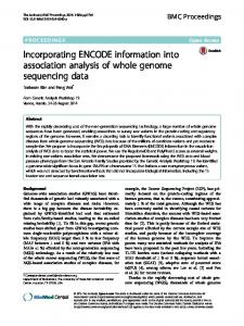
The temporal and spatial sequencing of events in the model is as follows. At the beginning of each period ‫ݐ‬, income growth is realized, bidding occurs and decisions to sell and convert land are made by the landowners and land developer respectively. Given land conversion in period ‫ݐ‬, ‫ܣ‬௜ is updated for every parcel i at the end of period ‫ݐ‬. At a given income level, the parcels with better proximity to urban centers, higher amenities, lower agricultural yields and lower conversion cost will become developed first. As land conversion proceeds, ceteris paribus, the reservation rent required by farmers (ܴ ∗ ) and the developer (ܴ ∗ + ‫ݔ(ܥ‬௜ )), will increase because parcels with low agricultural yields and conversion cost will be converted first. The residential rent for developable parcels will become less compared to the newly developed parcels because, ceteris paribus, parcels closer to urban centers and with higher amenities are developed first. However, income growth over time will also lead to higher rents paid on all parcels of developed land. Given income growth (i.e., g > 0), urban land rents will increase over time and additional agricultural land will be sold and developed for new residential use. In the absence of further income growth (g = 0), a static long run equilibrium is reached when the residential rent on any agricultural parcel i is insufficient to cover the reservation rent ܴ ∗ and the conversion cost ‫ݔ(ܥ‬௜ ).8 Simulation details and model results Given this specification of household and landowner behavior, we implement the model using a spatial simulation framework for Carroll County, Maryland, an exurban county located to the northwest of Baltimore MD and to the north of Washington DC (Figure 2). Carroll County 8

Because the stochastic term in the income is normally distributed, the income level in each period is unbounded. For simplicity, the stopping criterion for the long run static equilibrium is chosen so that the mean income level is insufficient to cover the threshold rent and the conversion cost. 28

was a predominantly rural county until 1960, at which point migration into the county began to increase. Between 1980 and 2000, population grew by 55% from just under 100,000 to over 150,000. This growth has resulted in the county shifting away from a predominantly agriculturebased landscape to one with a large portion of the landscape in developed land uses. The largest portion of the developed land is single-family residential dwellings. Since 1990, 95% of the development in the county has been some form of residential development (Wrenn 2011). Our goal is to provide an initial exploration of whether our model can explain the observed patterns of residential land use patterns in this study region. In particular, we observe a mix of fragmented and clustered residential development and persistent leapfrog development over time (Zhang et al. 2011). To operationalize the land conversion model for this landscape, we begin by creating a grid for the county defined by a cell size of 1݇݉ଶ. We use GIS data on land development patterns in Carroll County as of 1990 to initialize the model and overlay the 1km2 grid to generate the pattern of land development at this spatial resolution. We refer interchangeably to a land parcel i and cell i. As a first step in exploring the land use change pattern, we distinguish only between the developed and undeveloped land. All agricultural land is considered to be undeveloped land. The distinction among the residential, commercial, industrial land uses is ignored. Because the theoretical model is limited to a single density, size and type of developed land use, this simulation is clearly an oversimplification of the actual development process. Local land use amenities ‫ܣ‬௜ are calculated as the percentage of open space within the eight neighboring parcels for each parcel i. For instance, a parcel with four undeveloped neighbors has a value of ‫ܣ‬௜ = 0.5. As land development occurs in each time period, ‫ܣ‬௜ will also change for

29

some parcels and therefore ‫ܣ‬௜ is updated for each parcel i at the end of each round of simulated land conversion. In addition to this source of local spatial interaction among neighboring land parcels, three types of spatial heterogeneity are considered: the commuting cost which depends on the parcel’s accessibility to one or more urban centers; the agricultural yield, which determines the reservation rent of the farmers; and the conversion cost, which affects the site choice of the land developer. For each spatial variable, we calculated the aggregate values at this same 1km2 grid scale. Carroll County contains three small urban centers (Westminster, Syksville and Mt Airy). The City of Westminster located at the center of Carroll County and is the largest urban center in the county. Because many of the residents in Carroll County commute to Baltimore City and Washington D.C and their environs, we use the towns of Sykesville and Mt. Airy as proxy for these destinations. We calculate commuting costs as the sum of the distance from the centroid of each grid cell to each of these three destinations via the major roads network in Carroll County. Spatial variation in agricultural rents at the same scale are proxied using data on corn yields. This agricultural yield is obtained from the Soil Data Mart website (USDA) with corn chosen as the standard crop. The yield data are estimated values assuming that the land is subject to “a high level of management.” These values are observed at the spatial scale of soil type polygons. The 1km2 was overlaid in the soil polygons and an area-weighted mean yield value was derived for each grid cell. The conversion cost of each parcel is also based on these data. For each soil type in the Soil Survey Area (SSA) data, a rating is given that provides an indication of the soil’s suitability for urban development. This categorical rating was converted into a numerical value

30

and a mean value derived for each grid cell. All data were created using ArcGIS and imported into NetLogo to perform the model simulation.9 To operationalize the model, specification of preference, income and transportation cost parameters is necessary. First, we assume that residential migrants have a preference of the ௔

Cobb-Douglas form, ܷ(ܺ௜ ; ‫ܮ‬, ‫ܣ‬௜ ) = ܺ௜ భ (‫ܣ‬௜ ‫)ܮ‬௔మ , where the local amenity ‫ܣ‬௜ and the parcel size L are non-separable. For the baseline specification, we assume that ܽଵ = 0.8 and ܽଶ = 0.2. Second, based on our analysis of the 1990 and 2000 US Census income data for Carroll County, we parameterize income growth as a Brownian motion with drift g =0.5 and standard variation σ = 0.5.10 The initial income level is set at Y(t=0) = 6, which ensures that under the baseline specification the number of developed cells equals approximately the number of developed cells in the real landscape in year 2000. Next, we consider transportation costs. In Carroll County, the fuel cost of commuting is minimal. However, the opportunity cost of travel time can still be significant in determining the choice of location. We assume that the unit travel cost T = 2, so that the commuting cost is roughly 5% of the income. Lastly, we set the price for the composite good Px = 1 and the reservation utility level at U 0 = 2. The model is initialized with the 1990 land development pattern. The ending time of the simulation is chosen so that the number of developed parcels roughly equals the total number of developed patches in Carroll County in 2000.

9

For further details, see Chen (2009).

10

An annual income growth rate of 4% will generate roughly a 50% income growth at the end of 10th year. The sigma value implies that roughly 70% of the residents have an annual income growth in the range [−4%, 4%]. 31

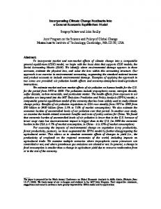
The averaged results of 100 simulations are summarized in the Table 1. Various approaches to model validation are possible. The simplest approach is to assume that if the location of a developed parcel in the simulation coincides with the location of a developed parcel in the real data, then it is considered to be a correct prediction. The total number of these parcels is reported in Table 1 as the number of correct predictions of “type A.” On average, the model simulations predict 40% of the parcels that are actually developed in 2000 correctly. However, this is a very stringent criterion for model validation. We relax this criterion to allow for near misses. Specifically, if the simulation predicts development of either the parcel that is actually developed in 2000 or at least one of the parcel’s immediate neighbors, then it is considered to be a correct prediction. The total number of these parcels is reported in Table 1 as the number of correct predictions of “type B.” On average, 80% of the developed parcels in the 2000 data has at least one neighboring parcel (or itself) that is developed in our simulation results. By comparison, given that 174 of 1,016 available cells are actually developed in Carroll County as of 2000, a completely random model of development generates a 17% chance of predicting the correct “type A” location of a developed cell that is observed in the real data and a 60% chance of predicting the correct “type B” location of a developed cell. Figure 3 illustrates the output from a representative model run and compares these to the aggregated urban land use pattern from 2000. Visual inspection shows some similarity between simulated pattern and the real pattern. However, closer inspection shows that in areas around the urban centers, the simulated land use pattern is not as clustered as the real land use pattern whereas in the areas away from urban center, it is not as scattered. To further compare the simulated land use pattern with that of the real data, several pattern metrics are generated using

32

the landscape metrics software package, Fragstats.11 To quantitatively measure land use pattern, we require measures that capture the characteristics of developed land use patches as well as measures that capture the spatial relation among different patches of development. For all developed land use patches, we calculate the mean area (m2), mean perimeter length (m) and the total number of patches for each simulation run. To measure the shape complexity of developed patches, we use the perimeter-area ratio index and the shape index. The perimeter-area ratio index is equal the ratio of the patch perimeter (m) to its area (m2). The shape index is calculated using a raster format. It is equal to the patch perimeter (measured in terms of the number of cells that comprise the perimeter) divided by the minimum perimeter possible (also measured in the number of cells) for a patch of the same area. In both cases, the higher the ratio, the more complex is the shape. In addition, we use the fractal dimension index to quantify the cross-scale regularity in the spatial pattern by measuring the relationship between the perimeter and the area across different sizes of patches. This measure is defined as two times the logarithm of the patch perimeter (m) divided by the logarithm of patch area (m2). A fractal dimension of greater than one indicates an increase in shape complexity. Finally, to capture the spatial relationship between the developed and undeveloped patches, the edge contrast index is used to measure the total amount of contrasting edges between developed and undeveloped land patches that share the same edge. The results from the observed and simulated landscapes are summarized in the Table 2. The first row specifies the pattern metrics used. The second row listed the values of the pattern metrics for the real land use pattern in 2000. The third row gives the mean value for the 100 simulations. The fourth row shows the standard deviation of the simulations. We find that the simulated land use pattern differs significantly from the observed land use pattern. Except for the 11

For a full discussion of these metrics, see McGarigal et al. (2002). 33

shape index, all pattern metrics for the real land use pattern lie beyond two standard deviation from those of the simulated patterns, suggesting that the probability for the model to regenerate the same metrics as in the data is approximately less than 10%. Discussion of model results and limitations In comparing the actual and simulated patterns of development, we find that the simulation model performs reasonably well in terms of predicting the location of exurban development, but that additional work is needed to reproduce these quantitative features of the observed land use pattern. For example, the model simulation generates too many patches and the patch sizes on average are too small. Nonetheless, the utility of this approach is evident. By developing a fully structural model of optimal household location demand and optimal land conversion by landowners and developers, this approach links the microeconomic foundations of land use with explicit predictions of land development and the evolution of land use patterns. Thus it is possible to explore how changes in underlying preference or cost parameters would be predicted to alter patterns of development. In so doing, this model is similar to other spatial simulation models that incorporate spatial dynamics and heterogeneity that are reviewed in the first part of this paper. Because we also rely on the simplifying assumption of a spatial equilibrium, the model presented here is most closely related to Caruso et al. (2007). Like the model results reported in Caruso et al. (2007), our model generates predictions of varying degrees of clustered and scattered urban land use patterns. However, unlike the model set-up in Caruso et al. (2007), we do not impose additional assumptions about market power and its transfer from a single migrant to the landowner. Instead, we maintain the assumptions of the spatial equilibrium model, in which market power resides with the landowner and households’ bids are always equal to their maximum WTP. For this reason, households are indifferent to 34

location, which, as we argued earlier, prevents us from assigning a specific household to a specific location. However, in this version of our model, all households are homogeneous and therefore it is not necessary to keep track of each household and its location. Instead, increasing residential land rents, which increase with income growth and are higher for more desirable locations (i.e., locations that are closer to the city and have higher amenities), determine the amount and location land conversion along with the landowner’s reservation rent and the land developer’s conversion costs. In a model with preference or income heterogeneity, an alternative approach would be needed since the spatial equilibrium assumption of utility indifference across all locations is no longer an appropriate assumption. Spatial arbitrage is possible as households sort themselves across locations and thus accounting for utility differences across space is necessary in order to identify sequential land conversion in space and time. This is much harder model to implement since we can no longer assume that a household’s bid is equal to the maximum WTP, i.e., ܾ(ܸ௜ ) ≠ ܸ௜ , and thus requires numerically evaluation of the household bid function in Equation (2). In addition to its continued reliance on the spatial equilibrium assumption, the most substantial limitation of the current model and its implementation is the lack of empirically estimated parameter values in the utility and cost functions. Ideally, one would derive an estimable model from the structural models of household location choice and land conversion decisions and estimate the parameters of the spatial simulation model in this way. Given a lack of data on household characteristics and land development costs, we are unable to do this in our current implementation of the model. However, such an approach is possible and certainly preferred to the calibration of parameters that we do here. However, empirical specification requires structural empirical estimation of the underlying behavioral models. While much 35

progress has been made recently in estimating structural household location choice models, these models still rely on static long run equilibrium assumptions. Dynamic models of household location and land development decisions are currently in their infancy (e.g., Bayer et al. 2010, Murphy 2007, Paciorek 2010) and extremely challenging to implement, given the data requirements and number of structural parameters to be estimated. Nonetheless, this approach to parameter specification of spatial simulation models holds much promise by marrying the empirical estimation of structural parameters with spatial simulation that is needed to evaluate non-marginal changes and spatial dynamic feedbacks. Concluding Comments Our review of models that incorporate greater spatial complexity highlights progress that has been made in incorporating spatial dynamics and spatial and agent heterogeneity into land market models. We discuss a few of the many challenges involved in developing such models, in particular the challenges of deriving optimal household and landowner bidding functions and market price formation from structural microeconomic models. We develop a model that provides a framework for a fully structural approach to modeling household bidding and price formation, but stop short of fully developing this model given the computational challenges involved. While there are many unanswered questions that remain, we conclude with a line of questioning that is critical if agent-based modeling is to take a firmer hold in economics. That is, how does the inclusion of specific agent-based model features that are ignored by the traditional spatial equilibrium models, such as short run transitional dynamics that arise from local interactions, alter the equilibrium predictions of the model? Since it is possible to use agentbased models to explicitly consider short run dynamics that are overlooked in the traditional 36

spatial equilibrium model, we should understand if and how these short run effects matter, e.g., do short run dynamics matter only for the transitional dynamics or if they also alter the long run equilibrium of the system? Does the system eventually reach a spatial equilibrium when such features are considered? And if so, is it the same spatial equilibrium as that which is achieved when these features are ignored and the spatial equilibrium is assumed to be instantaneously reached? And if not, under what conditions does the system diverge? Most importantly, does consideration of short run dynamics provide a more robust explanation of the changes in land markets or land use patterns that are observed in reality and not well explained by the traditional urban growth models? Exploration of such questions requires further improvements in agent-based models that make them comparable to the traditional urban economic models of land markets and land use patterns. Comparability requires: (i) rebidding, so that land prices can evolve over time with market conditions regardless of whether the land is occupied or not and (ii) that the household’s maximum value of the WTP function be equal to the household’s bid in spatial equilibrium. In addition, the household’s optimal bid should be derived from a fully structural model in which the optimal bidding process accounts simultaneously for the spatial variation at an individual plot level and market conditions that can deviate from those in spatial equilibrium. While none of the models we review here nor the model that we present accomplish all of these tasks, meaningful progress has been made. Much more work remains to develop agent-based models of land markets and spatial dynamics that can answer these and other questions, making this an exciting area for future research.

37

References Alonso, W. 1964. Location and Land Use: Toward a General Theory of Land Rent. Cambridge: Harvard University Press. Arnott, R.J. 1980. “A Simple Urban-Growth Model with Durable Housing.” Regional Science and Urban Economics 10(1), 53-76. Arnott, R. J. and F. D. Lewis 1979. “The Transition of Land to Urban Use.” The Journal of Political Economy 87(1), 161-169. Bayer, P. and C. Timmins. 2005. “On the Equilibrium Properties of Locational Sorting Models.” Journal of Urban Economics 57, 462-477. Bayer P, McMillen R, Murphy A, Timmins C. 2010. “A Dynamic Model of Demand for Houses and Neighborhoods.” Department of Economics, Duke University. Bayer, P., N. Keohane and C. Timmins. 2009. “Migration and Hedonic Valuation: The Case of Air Quality.” Journal of Environmental Economics and Management, 58, 1-14. Boucekkine, R., C. Camacho, and B. Zou. 2009. “Bridging the Gap between Growth Theory and The New Economic Geography: The Spatial Ramsey Model.” Macroeconomic Dynamics 13(1), 20-45. Brock, W. and A. Xepapadeas. 2008. “Diffusion-Induced Instability and Pattern Formation in Infinite Horizon Recursive Optimal Control.” Journal of Economic Dynamics & Control 32(9), 2745-2787. Capozza, D. and R. Helsley. 1989. “The Fundamentals of Land Prices and Urban-Growth.” Journal of Urban Economics 26(3), 295-306. Capozza, D. and R. Helsley 1990. “The Stochastic City”. Journal of Urban Economics 28(2), 187-203.

38

Caruso, G., D. Peeters, J. Cavailhes, and M. Rounsevell. 2007. “Spatial Configurations in a Periurban City. A Cellular Automata-Based Microeconomic Model.” Regional Science and Urban Economics 37(5), 542-567. Chen Y. 2009. “Three Essays on the Interactions Between Regional Development and Natural Amenities.” PhD Thesis. Ohio State Univerity. Chen, Y., C. Jayaprakash and E.G. Irwin. 2010. “Exurban Land Development with Short Run Dynamics.” Paper presented at the 2010 North American Regional Science Council Annual Meeting, Denver, CO, November 11-14, 2010. Desmet, K. and E. Rossi-Hansberg 2010. “On Spatial Dynamics.” Journal of Regional Science 50(1): 43-63. Ettema, D. 2011. “A Multi-agent Model of Urban Processes: Modeling Relocation Processes and Price Setting in Housing Markets.” Computers, Environment, and Urban Systems 35(1): 111. Epple, D. and H. Sieg. 1999. “Estimating Equilibrium Models of Local Jurisdictions.” Journal of Political Economy 107(4), 645-681. Filatova, T., D. Parker and A. van der Veen. 2009a. “Agent-Based Urban Land Markets: Agent”s Pricing Behavior, Land Prices and Urban Land Use Change.” Journal of Artificial Societies and Social Simulation. 12 (1). Available online: http://jasss.soc.surrey.ac.uk/12/1/3.html. Filatova T, van der Veen A, Parker D. 2009b. “Land Market Interactions between Heterogeneous Agents in a Heterogeneous Landscape: Tracing the Macro-Scale Effects of Individual Tradeoffs Between Environmental Amenities and Disamenities.” Canadian Journal of Agricultural Economics 57(4): 431-457.

39

Fujita, M. and P. Krugman. 1995. “When is the Economy Monocentric? Von Thünen and Chamberlin Unified.” Regional Science and Urban Economics 25(4), 505-528. Fujita, M. and H. Ogawa 1982. “Multiple Equilibria and Structural Transition of Nonmonocentric Urban Configuration.” Regional Science and Urban Economics 12, 161196. Irwin, E. G. 2010. “New Directions for Urban Economic Models of Land Use Change: Incorporating Spatial Dynamics and Heterogeneity.” Journal of Regional Science 50(1): 6591. Klaiber A, Phaneuf D. 2010. “Valuing open space in a residential sorting model of the Twin Cities.” Journal of Environmental Economics and Management 60(2): 57-77. Krugman P. 1991. “Increasing Returns and Economic Geography.” Journal of Political Economy, 99(3):483-499. Magliocca N, Safirova E, McConnell V, Walls M. 2010a. “Explaining Sprawl with an AgentBased Model of Exurban Land and Housing Markets.” Paper presented at the 2010 North American Regional Science Council Annual Meeting, Denver, CO, November 11-14, 2010. Magliocca N, McConnell V, Walls M, Safirova E. 2010b. “Zoning on the Urban Fringe: Results from a New Approach to Modeling Land and Housing Markets.” Manuscript. McGarigal K, Cushman SA, Neel MC, Ene E. 2002. “FRAGSTATS: Spatial Pattern Analysis Program for Categorical Maps.” Computer software program produced by the authors at the University of Massachusetts, Amherst. Available at the following web site: http://www.umass.edu/landeco/research/fragstats/fragstats.html Mills, E.1967. “An Aggregative Model of Resource Allocation In Metropolitan Areas.” American Economic Review 3, 129-144.

40

Miller, E., J.D. Hunt, J.E. Abraham and P.A. Salvini. 2004. “Microsimulating Urban Systems.” Computers, Environment, and Urban Systems 28, 9-44. Murphy A. 2007. “A Dynamic Model of Housing Supply.” Manuscript. Department of Economics, Duke University. Muth, R. 1969. Cities and Housing. Chicago: University of Chicago Press. Ogawa, H. and M. Fujita, 1980. “Equilibrium Land Use in a Nonmonocentric City.” Journal of Regional Science, 20, 455-475. Paciorek A. 2010. Supply Constraints and Housing Market Dynamics. Manuscript. Real Estate Department, Wharton School, University of Pennsylvania. Parker, D.C. and T. Filatova. 2008. “A Conceptual Design For A Bilateral Agent-Based Land Market With Heterogeneous Economic Agents.” Computers, Environment, and Urban Systems 32, 454–463. Parker, D.C., S.M. Manson, M.A. Janssen, M. Hoffmann and P. Deadman. 2003. “Multi-Agent Systems for the Simulation of Land Use and Land Cover Change: A Review.” Annuals of the Association of American Geographers 93(2), 314-317. Smith, M., J. Sanchirico, J. Wilen. 2009. “The Economics of Spatial-Dynamic Processes: Applications to Renewable Resources.” Journal of Environmental Economics and Management 57, 104-121. Smith, V.K., H. Sieg, H.S. Banzhaf, and R. Walsh. 2004. “General Equilibrium Benefits for Environmental Improvements: Projected Ozone Reductions under Epa's Prospective Analysis for the Los Angeles Air Basin.” Journal of Environmental Economics and Management 47, 559-584.

41

Tajibaeva L, Haight R, Polasky S. 2008. “A Discrete-Space Urban Model With Environmental Amenities.” Resource and Energy Economics 30(2), 170-196. Tesfatsion L, Judd K eds. 2006. Handbook of Computational Economics: Agent-Based Computational Economics. Volume 2. Amsterdam: North Holland. Turner, M. A. 2005. “Landscape Preferences and Patterns of Residential Development,” Journal of Urban Economics 57, 19-54. Thünen, von J. H.1826. De Isolierte Staat in Beziehung auf Landschaft und Nationalökonomie. Trans. By Wartenberg 1966 Von Thünen’s Isolated State. Oxford: Pergamon Press. Waddell, P., A. Borning, M. North, N. Freier, M. Becke and G. Ulfarsson. 2003. “Microsumulation of Urban Development and Location Choices: Design and Implementation of UrbanSim,” Networks and Spatial Economics 3, 43-67. Walsh, R.L. 2007. “Endogenous Open Space Amenities in A Locational Equilibrium.” Journal of Urban Economics 61, 319-344. Wrenn D. 2011. “Development Timing, Choice, and Pattern: Three Essays on the Conversion of Exurban Land.” PhD Thesis Draft. Ohio State University. Wu, J. and A. J. Plantinga. 2003. “The Influence of Public Open Space on Urban Spatial Structure.” Journal of Environmental Economics and Management 46, 288-309. Zhang W, Wrenn D, Irwin E. 2011. “New Metrics for Quantifying Spatial-Temporal Patterns of Leapfrog Development.” Manuscript.

42

Simulation result Mean Number of developed parcels 142 Number of correct prediction A 50 (%) (29) Number of correct prediction B 137 (%) (79) Number of developed parcels in 2000: 174

Min 126 41 (24) 128 (74)

Max 153 573 (33) 144 (83)

Std 5.2

3.7

Table 1: Model validation using “Type A” and “Type B” evaluation methods

Data 2000 Simulation (std) Data 2000 Simulation (std)

Data 2000 Simulation (std) Data 2000 Simulation (std)

Pattern at the county level Number of patches Mean area Total edges 39 2597 353000 48 2132 426750 (4.44) (207.60) (15197.00) Fractal dimension Perimeter-area ratio Shape index 1.02 32.9 1.27 1.03 35.4 1.31 (0.00) (0.67) (0.05) Pattern of the developed land use Number of patches Mean area Total edges 38 458 353000 47 306 426750 (4.40) (32.10) (15197.00) Fractal dimension Perimeter-area ratio Shape index 1.02 33.6 1.18 1.02 36 1.23 (0.00) (0.67) (0.04)

Edge contrast 91 96 (1.09)

Edge contrast 91.5 96.5 (1.08)

Table 2: Comparison of selected landscape metrics applied to simulated and actual land use patterns

43

EXOGENOUS SPATIAL HETEROGENEITY None

No Spatial Endogenous Feedbacks

Single source

Aspatial models of land use or land development (Arnott and Lewis 1979)

ENDOGENOUS SPATIAL FEEDBACKS

DYNAMIC** (evolving over time)

Interactions across spatial scales

Interactions at a single spatial scale

Static monocentric model (Alonso Monocentric model with 1964; Muth 1967; Mills 1969) or additional exogenous spatial dynamic monocentric model heterogeneity (Wu and Plantinga (Capozza and Helsley 1989, 1990) 2003) Interactions among local Interactions between households jurisdictions in a static equilibrium in a static equilibrium model with model with multiple city centers distance to a single city (Turner (Tajibaeva, Haight and Polasky 2005) 2008) Individual-neighborhood interactions in a static equilibrium model with neighborhood heterogeneity (Bayer et al. 2009; Klaiber and Phaneuf 2010; Smith et al. 2004; Walsh 2007)

Interactions at a single spatial scale STATIC (long run equilibrium)

Multiple sources

Interactions between individuals with exogenous change over time (Brock and Xepapadeas 2008, Boucekkine et al. 2009)

Individual-neighborhood

Interactions interactions of economic growth across spatial over time (Desmet and Rossiscales Hansberg 2010)

Individual-neighborhood interactions and landscape Individual-neighborhood heterogeneity in an agent-based interactions in an agent-based model without spatial equilibrium model in the absence of a spatial (Filatova et al. 2009b; Magliocca equilibrium with distance to city et al. 2010a,b); spatial simulation (Filatova et al. 2009a) model with exogenous population growth (Caruso et al. 2007; this paper)

Figure 1: Types of spatial complexity that have been incorporated into urban land market models ** Dynamic may refer to a process that is said to be a dynamic equilibrium or out of equilibrium. We do not distinguish between these for the purposes of this paper. 44

Carroll County

Baltimore Metropolitan Area

Baltimore City

Washington D.C.

Figure 2: Carroll County, MD

45

Figure 3a: Observed 2000 Carroll County

Figure 3b: Example of Simulated 2000 Carroll County

Urban Land Use Pattern

Urban Land Use Pattern

Note: The observed land use pattern is aggregated to a 1 km2 grid cell so that it is comparable to the model output at the same scale. In Figure 3a, dark cells indicate the location of predominantly developed land. In Figure 3b, dark cells indicate the location of land development as predicted by the model.

46