Incorporating Multiple Observations into Logistic Regression Models ...

ASA Section on Survey Research Methods

Incorporating Multiple Observations into Logistic Regression Models of Incident Disease 1

Julia L. Bienias 1,2, Phillip S. Kott4, Todd L. Beck 1, and Denis A. Evans 1,2,3 Rush Institute for Healthy Aging, and Departments of 2 Internal Medicine and 3Neurological Sciences, Rush University Medical Center, Chicago, IL, USA 4 National Agricultural Statistics Service, United States Department of Agriculture, Fairfax, VA, USA Contact: [email protected]

this paper, we follow Fuller (1975) and treat a real finite population as if it were a simple random sample from a conceptual infinite population. Combined with our sampling strategy, this allows us to estimate the model and randomization mean squared errors of parameters simultaneously. W e apply this approach to the Chicago Health and Aging Project (CHAP), a longitudinal communitybased study examining risk factors for chronic health problems of older adults. The CHAP design has two components, each conducted every three years. In the “census” component, all surviving members of the study population are interviewed and tested on a variety of health-related areas. In the sample component, a Poisson (stratified Bernoulli) sample is drawn from among the respondents to the full-population interview for detailed clinical evaluation and neuropsychological testing. To investigate risk factors for incident Alzheimer’s disease, a “disease-free” cohort is identified at the preceding time point and forms one major stratum in the sampling. W e describe the application of a delete-a-group jackknife mean-squarederror estimator to the modeling of risk factors for incident Alzheimer’s disease. Complicating matters is a sampling design that not only oversamples certain groups but also can contain data from the same individual more than once.

Abstract W e apply the delete-a-group jackknife variance estimator to a multi-wave longitudinal population-based study, the Chicago Health and Aging Project. This study examines risk factors for chronic health problems of older adults, particularly Alzheimer’s disease. Every three years, all surviving members of the study population are interviewed and a “disease-free” cohort is identified, from which a Poisson (stratified Bernoulli) sample is drawn for detailed clinical evaluation of incident disease at the next cycle. W e show how multiple observations from the same individual can be incorporated into an analytic model and how the deletea-group jackknife can be used for variance estimation. KEY W ORDS: Complex surveys, Poisson sampling, Randomization-based inference, Longitudinal, Alzheimer’s disease 1. Introduction Complex sampling designs present particular challenges to statistical modeling and estimation. In social, economic, and health research, samples of individuals are typically taken for more detailed followup when the cost of collecting such data on all the individuals in the study is cost-prohibitive. In such studies, the estimands of interest are typically model parameters or measures of association, rather than means or totals. Complex sampling plans are often used in this context to guarantee the inclusion of certain subgroups of the population under study or increase the number of sampled individuals with known or suspected predictive variables of interest. In studies of risk factors of incident disease, for example, analysts often increase the sample number of expected cases of diseases by oversampling groups expected to exhibit more incident disease. Inference under complex sampling plans can be model-based (as in B reckling et al. 1994) or randomization-based (as in Binder 1983). W hen the estimands of interest are model parameters, Binder and Roberts (2003), among others, have shown that using randomization-based techniques can often produce inferences robust to certain types of model failure. In

2. Design of the Study 2.1 Overview The Chicago Health and Aging Project (CHAP) is an ongoing longitudinal community-based cohort study of older adults (65 years of age and older) living in a geographically defined area of Chicago, Illinois. The study was approved by the Institutional Review Board of Rush University Medical Center. Data for CHAP are collected during face-to-face interviews from participants who have given written, informed consent; we will call these participants the study population. The primary purpose of CHAP is to investigate risk factors for common chronic conditions of older adults, with a particular emphasis on risk factors for decline in cognitive functioning and incident Alzheimer’s disease. First identified in the early

2767


twentieth century by Dr. Alois Alzheimer (Alzheimer 1907), dementia of the Alzheimer’s type is a particularly debilitating progressive neurodegenerative disorder, characterized by declines in memory and other cognitive processes. It currently has no known cause and no cure, although some partial symptomatic treatments exist. Because of its long-term nature and the changing age structure of the population in the U.S. and other industrialized countries, it is projected that the cost of treatment and care for those with Alzheimer’s disease will place increasingly high demands on the health-care system (Hebert et al., 2003, 2004). Thus, the identification of potentially modifiable risk factors is of great public health concern. Since the inception of CHAP in 1993, approximately 10,000 older adults have been enrolled into the study. In-home interviews are conducted with all surviving participants approximately every three years. W e will refer to these waves of data collection as “cycles.” Interviews include performance-based tests of physical and cognitive function as well as structured questions about sociodemographic characteristics, health, and lifestyle. In addition, a random sample of individuals is taken from each cycle of study-population interviewing. Sampled individuals are asked to participate in an additional interview, a detailed clinical evaluation that includes neuropsychological and neurological evaluation for Alzheimer’s disease. The sample taken from the first, or baseline, cycle provided estimates of prevalent disease. Samples taken from later cycles allow us to examine incident disease. In do this, a “disease-free” cohort is identified at the preceding time point and forms one major stratum in the sampling. Further details of the study and the design are available in Bienias et al. (2003a) and W ilson et al. (1999). In this paper, we will focus on aspects of the design involving the samples taken for clinical evaluation of incident Alzheimer’s disease.

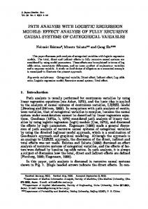
evaluation for incident disease. Figure 1 illustrates the design schematically. The solid black arrows, which extend from the time of the baseline interview to the time of the first evaluation for incident disease, represent the first incidence sample. The second set of arrows (dots and dashes) represent the second sample. Note that some of the sample is new, and some is a continuation of the old (solid line) sample. The third set of arrows (dotted lines) are included to show the continuation of the design into the future. The length of each arrow is approximately 3 years by design. W e focus here on the combined sample drawn after the second (solid lines) and third (dots and dashes) fullpopulation interview cycles. Some individuals identified as eligible to be sampled provided two observations to the combined sample; some only one, and many none at all.

Figure 1. Schematic Representation of Sample Design. 2.3 Sample Selection Each sample of individuals for clinical evaluation was chosen using the same basic approach. People were identified as belonging to strata defined by the cross-classification of race (black or non-black), sex, age group (in 5- or 10-year groupings), and cognitive performance (based on four tests given to all individuals in the study-population interview). Additionally, for the second incidence sample, we also stratified by whether or not an individual had been a participant in the first incidence sample. The strata used in sample selection were not technically design strata in the customary meaning of the term in the survey-sampling literature. W ithin each “stratum,” individuals were selected into the sample using Bernoulli sampling, that is, independently, with the same probability of selection applied to each member of the stratum. Stratified Bernoulli sampling is a special case of Poisson sampling.

2.2. Successive Samples for Incident Disease Based on brief tests of cognitive performance given to all participants and further information from the first (baseline) clinical evaluation, a cohort of persons believed to be free of Alzheimer’s disease was identified. Approximately three years later, following the second cycle of full-population interviews, a sample of those persons free of disease at baseline was taken for the first clinical evaluation for incident disease. Repeating the process, at this second cycle, a new cohort of persons believed to be free of Alzheimer’s disease was identified. Approximately three years later, following the third cycle of study-population interviews, a sample of this second cohort was taken for

2768


estimator for B, which in turn will serve as an estimator for the model parameter $. The above reasoning supposes we assume the logistic model (1) holds for all the putative observations in the analytical universe U. Alternatively, we can treat B as the definition of a finite-population parameter, and try to estimate it using randomizationbased survey sampling theory. If b solves the samplebased score equation, 3 3 X it[Y it ! f(X it b)]( *it /Bit) = 0, (3) i 0 PN t 0 Ui then it can be both a consistent estimator for $ under the logistic model and for B under randomization-based theory. Binder and Roberts (2003) make a similar point. Their concern is asymptotic unbiasedness under either model- or randomization-based inference rather than consistency. Establishing dual consistency requires some additional mild assumptions we assume to hold in our context. Randomization-based theory is appealing because it frees us from making assumptions about models. Unfortunately, its results are constrained to the population under review, in this case the universe of putative observations for the eligible CHAP population. This is extremely limited. Rather, we believe that other populations of older adults will have similar risk factordisease associations, which is why we are studying the behavior of the CHAP population W ith this in mind, we follow Fuller (1975) and treat the individuals in the eligible population, P N, as a simple random sample of a conceptual infinite population. The goal of randomization-based inference is now not to estimate the finite-population parameter, B, but its limit, say B*, as N grows arbitrarily large in a well-defined way. The score equation for b in (3) is a consistent estimator for B* under mild conditions. Note there is no need to include an additional probability-ofselection factor in equation (3) to reflect the sampling of the eligible population from the conceptual infinite population, because these probabilities of selection are the same for all individuals and thus for all putative observations associated with them. W hen the model in (1) holds, B* = $ in probability under mild conditions. This is true even when the sampling design is nonignorable (Rubin, 1976) in the sense that observations in the sample behave differently from those outside of it, and E( ,it|X it, *it) 0. The CHAP design may be nonignorable if there is relevant information about the risk of disease contained in the probabilities of selection that is not captured by (1). W e can go even further.The limit of the finitepopulation parameter B is the model parameter $ whether or not E( ,it | X it) = 0. This conditional expectation is usually a requirement of the model. In

3. Statistical M odeling of Risk Factors for Disease Incidence Let P N be the subset of N individuals in the CHAP study population eligible for sampling into the first or second incident clinical-evaluation samples or both, and let i index an individual in this set. W e call P N the eligible population. In principle, we could observe a clinicalevaluation measurement whenever individual i was in the eligible population. Let U i be the set of such putative observations for i. This set can have 1 or 2 members, depending on whether individual i was eligible once or twice. The population we want to analyze here is U, the union of the U i, that is, the set of all putative observations. W e call U the analytical universe. The term “universe” is used to distinguish this population of putative observations from a population of individuals. Let *it = 1 if individual i is in the tth clinicalevaluation sample, and *it = 0 otherwise, where Bit is the probability of person i being selected for the tth sample. Note that E( *it) = Bit. Let n be the number of individuals with actual observations in the two incident clinical-evaluation samples combined and m be the total number of observations: n # m # 2n. Because the study was designed such that each individual in the incident sample was observed for approximately three years between entry into the sample and clinical evaluation for the presence of disease, we used logistic regression to examine risk factors for incident disease. Let Y it denote the presence (=1) or absence (=0) of disease at time point t for individual i. Let X it = (X it1, ..., X itJ) denote a row vector containing a set of J covariates for i, to be associated with the clinical evaluation at time t. Typically, because we are interested in assessing the effect of risk factors for disease, the values of these covariates will be taken at the ascertainment of disease-free status from the preceding cycle. Suppose we assume that the Y it in the population satisfy this logistic model: Y it = f(X it$) + ,it, (1) where f(X it$) = [1 + exp( !X it $)] -1 , $ = ($1, ..., $J)' is an unknown vector of parameters, and ,it is a random variable with E( ,it|X it) = 0. The ,it are assumed to be uncorrelated across individuals but not necessarily across putative observations for the same individual. Using maximum likelihood principles, a consistent estimator for $ under mild conditions is the vector B that satisfies 3 3 X it [Y it ! f(X itB)] = 0 (2) i 0 PN t 0 Ui (see McCullagh and Nelder, 1989). In practice, however, we only know the Y it values for observations in the sample. Consequently, we need a sample-based

2769


b ! B* . T -1 (1/m) 3 E i , where i 0 PN T = plim {(1/m) 3 3 X it'X it f'(X itB*)( *it /Bit)} i 0 PN t 0 Ui and f'(z) = df(z)/dz = f(z)[1 ! f(z)]. The randomization MSE of b is the randomization expectation of mse(b) . T -1 (1/m 2) 3 E i E i ' T -1. . (5) i 0 PN The right hand side of equation (5) cannot be calculated because T and the E i are unknown; one way to estimate the randomization mean squared error of b is to follow Binder and replace T and the E i with sample analogues. A popular alternative to Binder’s approach is to use a replication method. As in Bienias et al. (2003b), we follow this second path and compute a delete-a-group jackknife (Kott 2001, 2005). This is done by randomly assigning the individuals in P N into G mutually exclusive groups of nearly equal size. Letting *it(g) = *it when individual i is not in group g and 0 otherwise, we can define b (g) as the solution to 3 3 X it[Y it ! f(X itb (g))] ( *it(g) /Bit) = 0. i 0 PN t 0 Ui Only those data that form the complement of a given group g are included, that is, we “delete the group.” A delete-a-group jackknife estimator for the randomization mean squared error of b is G mse dag(b) = [(G-1)/G] 3 (b (g) ! b)(b (g) ! b)'. (6) g=1 It is not hard to show that under mild conditions mse dag(b) is an almost randomization unbiased estimator for mse(b), which in turn is an almost unbiased estimator for the randomization MSE of b. W hen the sampling design is ignorable and the standard logistic model holds, so that E( ,it|X it, *it) = 0, mse dag(b) is also an almost unbiased estimator for the model MSE of b as an estimator for $. The reasoning behind this assertion replaces E i in equation (4) by u i = 3 X it[Y it ! f(X it$)] ( *it /Bit) t 0 Ui = 3 X it ,it ( *it /Bit). t 0 Ui The model independence of the u i rests on the ,it |X it being uncorrelated across individuals but not necessarily observations. The remainder of the argument parallels the randomization case with T replaced by the sample value (1/m) 3 3 X it'X it f'(X itB*)( *it /Bit). Alternatively, consider a robustified general logistic model where only the X it ,it have zero means and are uncorrelated across individuals, so that $ = B* in probability. Then, mse dag(b) is an almost unbiased estimator for the sampled-weighted average – that is, the randomization expectation – of the model mean

the standard formulation of the logistic model, d{logit[E(Y it)]}/dX it, is assumed to be constant and equal to $ across all realizations of X it. That means that a unit change in X itj leads to an (exp{ $j}-1)x100 .$j x100 percent change in the odds of Y it being 1 no matter what the values of the components of X it. W hen the population and model is such that E( ,it|X it) 0 for all X it, the standard assumption can be replaced with a more general one: E(X it ,it) = 0. Such a generalization reinterprets the meaning of $ to be the average value for M{logit[E(Y it)]}/MX it across the universe of X it values. Consequently, a unit change in X itj leads to an approximate $j x100 percent change in the odds of Y it being 1 on average. T he ra nd om izatio n-b ased techniq ue of incorporating the sampling weights, *it /Bit, into the determination of b, which is often given a model-based justification when the sampling design is nonignorable, also provides a means of estimating our robustified model parameter. 4. The Delete-a-Group Jackknife M ean-Squared-Error Estimator W e describe an estimator for the randomization MSE of b as an estimator for B*, which also serves as a measure of the model MSE of b as an estimator for $. For the remainder of this discussion, we will discontinue using the clarifying, but unwieldy, phrase “as an estimator for B*” when referring to randomization-based properties of b. We focus on mean squared error rather than variance because b is a randomization-consistent estimator but not necessarily a randomization-unbiased one. Under mild conditions, however, the randomization bias is an asymptotically insignificant contributor to the randomization mean squared error of b. Consequently, the randomization variance and MSE of b are asymptotically identical. Effectively, we have a two-stage sample. In the first stage, a simple random sample of individuals eligible for either clinical-evaluation study is drawn from the conceptual infinite population of such individuals. The result of this (imaginary) stage of sampling is the finite eligible population, P N. In the second (real) stage, a Poisson subsample of observations is drawn. For each i 0 P N, let E i = 3 X it[Y it ! f(X itB*)] ( *it /Bit). (4) t 0 Ui As P N is a simple random sample from a conceptual infinite population, the E i are uncorrelated random variables with mean zero, just as if they had been sampled with replacement. Consequently, under mild conditions, we can parallel Binder (1983) and write

2770


squared error of b as an estimator for $. The key here is the near equality of E * {E ,[(b ! $) 2]} and E , {E *[(b ! B*) 2]}, where the subscripts * and , refer to randomization and model-based inference, respectively.

the Cycle 2 sample plus and the 299 persons who had their first clinical evaluation in the Cycle 3 sample). Initially, we ignored nonresponse, which is implicitly the same as assuming nonrespondents were missing completely at random. As a sensitivity analysis to the effect of missing data, we re-analyzed the same two data sets but with sampling-weight adjustments for nonresponse computed using a propensity-stratification approach (Rosenbaum and Rubin 1983; Little 1986; Eltinge and Yansaneh 1997). W e first found the bestfitting logistic regression model for predicting response in each of the samples by building up a set of individual predictors that included demographic characteristics and measures of physical, cognitive and mental health. W e then created ten cells based on deciles of the fitted logistic response probabilites for each sample, for a total of twenty adjustment cells for the combined sample. W ithin a cell, the nonresponse adjustment factor was the inverse of the weighted response rate. In like manner, the nonresponse adjustment factors were computed separately for each replicate. The final weight for analysis was the sampling weight times the nonresponse adjustment factor. The adjustment factors ranged between 1.051 and 2.114 for the full combined sample of 1,346 observations and between 1.185 and 2.763 for the smaller sample of 1,134 unique persons.

5. The Application 5.1 Statement of the Problem W e considered models for incident Alzheimer’s disease, adjusting for time-on-study, demographic variables (e.g., age, sex) and other key covariates as appropriate for the given risk factor of interest. We present two models: (a) a simple model with time-onstudy and age, and (b) the final risk-factor model reported in Evans et al. (2003). Evans et al. (2003) examined the effect of the presence or absence of the ,4 allele of the apolipoprotein E gene, a known risk factor for Alzheimer’s disease, and whether or not the magnitude of its effect varied by race. The models reported in that paper were estimated from the first incidence sample from the CHAP study (the Cycle 2 sample; schematically, the solid-line arrows in Fig. 1). W e chose to use logistic regression, adjusting for time-on-study, in preference to survival models, for two reasons: (1) There is a long time between measurements (three years by design, sometimes longer in practice), which would induce interval censoring, and (2) Although in practice there is some variability in timeon-study across persons, the study is designed to have essentially the same length of follow-up for everyone. W e estimated the variances with SAS® using custom software we wrote (Bienias, 2001) and used 100 groups (G=100 in Eq. (6)) to support the asymptotic normality assumptions inherent in statistical testing.

5.3 Results W e first considered models predicting the probability of Alzheimer’s disease based on age at entry into the particular observation period (centered at the approximate mean of 75 years) and time during that observation period. For the Cycle 2 sample, this is the age at the time a person was determined to be free of disease in conjunction with the first data collection cycle. Similarly, for the Cycle 3 sample, this is age at the second data collection cycle. “Time on study” is the time between eligibility for the given sample and clinical evaluation for incident disease. Table 1, Model A, shows the estimates and standard errors for this simple model for our four data sets. As we expect, the effect of age is strong and very significant (all W ald test |t99|s > 7.000, all ps < 0.001), whereas the effect of time on study is not at all significant (all |t99|s < 0.212, all ps > 0.833), as we would hope and consistent with results reported previously (Wilson et al. 2002). W e next considered estimates for the primary riskfactor model reported in Evans et al. (2003, Table 2, first model, p. 187). Table 1, Model B, contains the parameter estimates and standard errors from that paper and from our four analytic data sets. Age was as just defined for the first set of models, and education was centered at the approximate mean of 12 years. Race was based on self-report and coded 1 for black and 0

5.2 Summary of the Analytic Data Sets As mentioned earlier, an individual can contribute one or two observations to the analyses described here. A total of 1,249 persons were selected for the Cycle 2 sample, and a total of 712 persons were selected for the Cycle 3 sample, of whom 314 had also been selected at Cycle 2. W e have a total of 1,134 persons contributing 1,346 observations to our analyses; 623 persons contributed only to the first (Cycle 2) sample, 299 persons contributed only to the second (Cycle 3) sample, and 212 persons contributed to both samples. The response rates, weighted to the frame, among survivors still living in the community were 77.4% for the Cycle 2 sample and 72.8% for the Cycle 3 sample. W e considered two separate data sets: (a) The fully combined samples just described (1,346 observations), and (b) A subset using only one observation from each of the 1,134 persons (i.e., all of the observations from

2771


for non-black; in the full study population, only 0.2% of participants reported another race. Apoliprotein E was the presence (=1) or absence (=0) of the ,4 allele. As we see in Table 1, M odel B, the estimates and the standard errors are fairly stable across the four data sets (Columns 1 - 4). The estimate for sex varies somewhat but is never close to statistically significant (all ps > 0.39). Comparing the estimates from the combined samples to that previously reported in Evans et al. (2003) (Column 5 on Table 1), we see the estimates are mostly similar. Given that the addition of later samples can shift the population distribution of the demographic variables associated with the analytical universe, some differences are to be expected. For example, realizing that women have a longer expected life span than men, we expect the eligible population (from which the analytical universe of observations is derived) to contain more women as time goes on. Reassuringly, the impact of nonresponse on our estimates of risk factors and covariates of interest does not appear to be meaningful, as evidenced by the high degree of similarity of the estimates between models with and without nonresponse adjustment (i.e., between Cols. (1) and (2) and between Cols. (3) and (4)). We see this for the simple and the complex models. Some may be surprised that explicit nonresponse adjustment, although leading to more variability in the weights, did not appear to uniformly increase s.e. estimates. W e also note the parameter estimates for age and their estimated standard errors from the simple models presented in Table 1 are very similar to the estimates in the corresponding complex models (Table 2). Finally, the more data for estimation, the sharper the estimates. As the number of sampled observations increases from the single sample reported in Evans et al. (2003) through the single-observation-per-individual to the full-sample analysis, standard errors tend to decrease.

nonignorable sample design (in which equation (1) holds but E( ,it | X it, *it) 0) and the failure of the standard model assumption (in which E( ,it | X it) must be zero). W hen the standard model fails, however, the estimated model parameters are effectively averages, in our case taken across putative observations in the eligible population. As such, they apply approximately to populations with covariate values similar to CHAP. Using conventional stratified simple random sampling has some apparent advantages over our stratified Bernoulli design. Domain sample sizes can be targeted better and estimated parameters may be more efficient (when E( , it) varies across the strata). The problem with conventional stratified sampling when analyzing survey data is that the stratum population sizes may themselves need to be treated as random variables. If so, Korn and Graubard (1998) show that randomization-based techniques developed for finite populations may not have the appropriate model-based properties. Fuller’s idea of treating the finite population as a simple random sample from a conceptual infinite population does not always allow the analyst to ignore the finite population correction factors of randomization-based theory. It does, however, when the actual selection mechanism linking the finite population to the sample is Poisson. The delete-a-group jackknife provides a simple means for estimating the variances in a sample containing more than one observation from the same population unit. Our design and methodological approach have several strengths. As just mentioned, under Poisson sampling, we can ignore the finite population correction (fpc) factor. Although in many design settings such as national household surveys, fpc is effectively ignorable because of very small sampling fractions, in an epidemiological study such as CHAP, probabilities of selection are set much higher to allow researchers to examine as many members of the population as possible within budgetary constraints. Thus our ability to ignore fpc greatly simplifies computations as well as giving us a more realistic mean-squared-error estimate. Second, the approach can be applied cross-sectionally as well as longitudinally, for example, when multiple samples are taken from a given list frame for different studies but there is a desire to combine those samples at a later date for a particular analysis. Third, our methodology can be adapted to the analysis of other types of modeling beyond logistic regression. Finally, being able to combine samples as we describe allows for a substantially more efficient use of the study population. For example, when studying older populations, we expect some loss to follow-up due to decease over the life of a longitudinal study. Being able to combine samples across time allows us to make better use of the

6. Discussion As we have shown, the delete-a-group jackknife variance estimator can be useful in settings where standard techniques are not applicable or difficult to implement. In our Chicago Health and Aging Project application, this complexity arose as a consequence of our wanting to target particular domains of individuals in each sampling cycle and to combine observations across cycles involving overlapping sets of individuals. By employing stratified Bernoulli sampling, we were able to target domain sample sizes for each cycle of sampling while at the same time assuring the independence of observations from different individuals. This allowed us to conduct a randomization-based analysis that also served as a robust model-based one: robust against both a

2772


data, as well as giving us an opportunity to study temporal or cohort effects. In CHAP, we are extending the methodology to future repeated sampling of the original study population and to newly added cohorts.

Nonresponse in the U.S. Consumer Expenditure Survey.” Survey Methodology, 23, 33-40. Evans, D. A., Bennett, D. A., W ilson, R. S., Bienias, J. L., Morris, M. C., Scherr, P. A., Hebert, L. E., Aggarwal, N., Beckett, L. A., Joglekar, R., BerryKravis, E., and Schneider, J. (2003). “Incidence of Alzheimer’s Disease in a Biracial Urban Community: Relation to Apolipoprotein E Allele Status.” Archives of Neurology, 60, 185-189. Fuller, W . A. (1975). “ Regression Analysis for Sample Surveys.” Sankhy ~, Series C, 37, 117-132. Hebert, L. E., Scherr, P. A., Bienias, J. L., Bennett, D. A., and Evans, D. A. (2003), “Alzheimer’s Disease in the US Population: Prevalence Estimates Using the 2000 Census.” Archives of Neurology, 60, 1119-1122. Hebert, L. E., Scherr, P. A., Bienias, J. L., Bennett, D. A., and Evans, D. A. (2004). “State-Specific Projections through 2025 of Alzheimer’s Disease Prevalence.” Neurology, 62, 1645. Korn, E. L. and B. I. Graubard, (1998), “Variance Estimation for Superpopulation Parameters,” Statistica Sinica, 8, 1131-1151. Kott, P. S. (2001). “The Delete-a-Group Jackknife.” Journal of Official Statistics, 17, 521-526. Kott, P. S. (2005). “Delete-a-Group Variance Estimation for the General Regression Estimator under Poisson sampling.” Journal of Official Statistics, to appear. Kott, P. S. and Stukel, D. M. (1997). “Can the Jackknife be Used with a Two-Phase Sample?” Survey Methodology, 23, 81-89. Little, R. J. A. (1986). “Survey Nonresponse A d ju stm e nts fo r E stim ates of M e a ns.” International Statistics Review, 54, 139-157. McCullagh, P., and Nelder, J. A. (1989). Generalized Linear Models (2 nd Ed.). London: Chapman and Hall. Rosenbaum, P. R., and Rubin, D. B. (1983). “The Central Role of the Propensity Score in Observational Studies for Causal Effects.” Biometrika, 70, 41-55. Rubin, D. B. (1976). “Inference and Missing Data.” Biometrika, 63, 581-590. W ilson, R. S., Bennett, D. A., Beckett, L. A., Morris, M. C., Gilley, D. W ., Bienias, J. L., Scherr, P. A., and Evans, D. A. (1999). “Cognitive Activity in Older Persons from a Geographically Defined P o p u la tio n .” J o u r n a l o f G e ro n to lo g y : Psychological Sciences, 54B, P155-P160. W ilson, R. S., Bennett, D. A., Bienias, J. L., Aggarwal, N. T., Mendes de Leon, C. F., Morris, M . C., Schneider, J. A., and Evans, D. A. (2002). “ Cognitive Activity and Incident Alzheimer’s Disease in a Population-Based Sample of Older

7. Acknowledgments Support for this work was provided, in part, by a grant from the United States National Institutes of Health, National Institute on Aging, RO1-AG11101. The views expressed in this article are those of the authors and do not necessarily reflect those of the U. S. National Agricultural Statistics Service. SAS is registered trademark of SAS Institute Inc. in the U.S. and other countries; ® indicates U.S. registration. W e thank Ann Marie Lane for community development and oversight of the CHAP project coordination; Michelle Bos, Holly Hadden, Flavio LaMorticella, and Jennifer Tarpey for coordination of the CHAP study; George Dombrowski for data management; and W oojeong Bang for assistance with programming. 8. References Alzheimer, A. (1907). “Uber eine eigenartige Erkrankung der Hirnrinde,” Allg. Z. Psychiatr. Psych. Gerichtl. Med., 64, pp. 146-148; translated by Jarvik, L., and Greenson, H., 1987, Alzheimer Disease and Associated Disorders, 1, 7-8. Bienias, J. L. (2001). “Replicate-Based Variance Estimation in a SAS® Macro.” Proc. of the Fourteenth Annual Meeting of the NorthEast SAS Users Group, 727-735. [See www.nesug.org.] Bienias, J. L. Beckett, L. A., Bennett, D. A., W ilson, R. S., and Evans, D. A. (2003a). “Design of the Chicago Health and Aging Project (CHAP).” Journal of Alzheimer’s Disease, 5, 349-355. Bienias, J. L., Kott, P. S., and Evans, D. A. (2003b). “Applying the Delete-a-Group Jackknife Variance Estimator to Analyses of Data from a Complex Longitudinal Survey.” Proceedings of the Annual Meeting of the American Statistical Association, Section on Survey Research Methods [CD-ROM]. Alexandria, VA: American Statistical Association. Binder, D. A. (1983). “On the Variances of Asymptotically Normal Estimators from Complex Surveys.” Int’l. Statistical Review, 51, 279-292. Binder, D. A. and Roberts, G.R. (2003). “DesignBased and Model-Based M ethods for Estimating Model Parameters.” Analysis of Survey Data, Chambers, R.L. and Skinner C.J. (eds). New York: W iley, 29-48. Eltinge, J. L., and Yansaneh, I. S. (1997). “Diagnostics for Formation of Nonresponse Adjustment Cells, with an Application to Income

2773


Persons.” Neurology, 59, 1910-1914. Table 1. Model Parameter Estimates (Standard Error Estimates) for Simple (A) and Complex (B) M odels Data Used (1) Both Cycle 2 and Cycle 3 Clinical Evaluations

(2) (1) but with Nonresponse Adjustment

(4) (3) but with Nonresponse Adjustment

(5) Cycle 2 Clinical Evaluation CE Only (from Evans et al. 2003)

Intercept

-2.212 (0.515)

-2.216 (0.497)

-2.178 (0.584)

-2.062 (0.630)

n/a

Time on Study (years)

0.015 (0.122)

0.025 (0.118)

0.017 (0.138)

-0.007 (0.146)

n/a

Age (years-75)

0.127 (0.015)

0.127 (0.016)

0.137 (0.016)

0.133 (0.019)

n/a

Intercept

-2.885 (0.567)

-2.915 (0.548)

-2.825 (0.629)

-2.664 (0.691)

-2.99 (0.746)

Time on Study (years)

0.058 (0.120)

0.070 (0.117)

0.055 (0.136)

0.015 (0.149)

0.108 (0.131)

Age (years-75)

0.131 (0.017)

0.133 (0.018)

0.142 (0.018)

0.140 (0.021)

0.152 (0.024)

Male Sex

0.177 (0.242)

0.204 (0.238)

0.039 (0.266)

0.122 (0.285)

-0.112 (0.341)

Black Race

0.610 (0.371)

0.634 (0.385)

0.762 (0.398)

0.815 (0.418)

0.612 (0.467)

Education (years-12)

-0.096 (0.047)

-0.091 (0.051)

-0.090 (0.051)

-0.073 (0.060)

-0.131 (0.051)

Presence of an Apoliprotein E ,4 Allele

0.953 (0.395)

0.886 (0.371)

0.912 (0.430)

0.778 (0.402)

1.066 (0.334)

Black Race * ,4

-1.039 (0.540)

-1.042 (0.530)

-1.164 (0.604)

-1.156 (0.588)

-1.062 (0.555)

Model Term

Model A

Model B

2774

(3) Both Cycle 2 and Cycle 3 Clinical Evaluations, one obs./person