Incorporating Spatial Dependencies in Random Parameter Discrete Choice Models
Abolfazl (Kouros) Mohammadian Department of Civil and Materials Engineering University of Illinois at Chicago 842 W. Taylor St. Chicago, Illinois 60607-7023 Tel: (312) 996-9840 Fax: (312) 996-2426 Email:
[email protected] Murtaza Haider School of Urban Planning and Dept. of Civil Engineering McGill University 815 Sherbrooke Street West, Suite 400 Montreal, Quebec, Canada Tel: (514) 398-4079 Fax: (514) 398-8376 Email:
[email protected] Pavlos S. Kanaroglou School of Geography and Geology McMaster University Hamilton, Ontario, Canada Tel: (905) 525-9140 Ext. 23525 Fax: (905) 546-0463 Email:
[email protected]
Paper submitted for presentation at the 84th Annual Transportation Research Board Meeting January 2005 Washington D.C.
Abstract This paper presents the process of derivation and development of a spatial choice model. A mixed (random parameter) spatial multinomial logit model is formulated that incorporates spatial dependencies to predict type choice for new housing projects. The results of the model suggest that type choice of a housing project is influenced by other projects in adjacent zones, resulting in correlated choice behavior over space. Heterogeneity effects also found to be an important factor in this model. The results of the model present a substantial improvement, in terms of model fit, over multinomial logit and standard spatial logit models.
Keywords Spatial Dependency, Mixed Logit, Spatial Logit Model, Housing Choice
1. Introduction Land-use models as well as housing choice models deal with space and time resulting in spatial and temporal dependencies across decision-makers and alternatives. While researchers often account for temporal autocorrelation in their models, spatial autocorrelation is frequently ignored in discrete choice models, leading to inconsistent estimates (McMillen, 1995). One reason behind this might be the fact that space is in general more complex to deal with than time. While time is one-dimensional, space in its simplest form, is two-dimensional. If spatial dependencies exist, it can be argued that decision-makers may influence each other, resulting in correlated choice behavior over space. It can be shown that proximity to other decision-makers in space influences the decision process and in fact this influence increases with proximity. Early attempts to estimate models of spatial dependence used continuous random variables, in the context of regression analysis (Anselin, 1988; Case, 1992; Dubin, 1992 and 1998). There has been relatively little work in the literature on incorporating spatial dependencies into discrete choice models. Boots and Kanaroglou (1988) incorporated the effect of spatial structure in discrete choice models of migration. Few other studies investigated spatial effects in conventional probit models developed on binary data where spatial dependencies were present (McMillen, 1995; Berton and Vijverberg, 1999). Dubin (1995) developed a spatial binary logit model to predict the diffusion of a technological innovation. In her model, the probability of adoption of a new technology varies with the firm’s own characteristics and its interactions with previous adopters. Paez and Suzuki (2001) tested the application of this spatial binary logit model to a land use problem considering the effects of transportation on land use changes. Mohammadian and Kanaroglou (2003) expanded the binary choice model into a more general form and derived a spatial multinomial logit model (SMNL) and tested it on a housing type choice problem. In this paper, spatial dependency terms are implemented in a mixed (random parameter) logit framework to form a spatial mixed logit model (SML) allowing coefficients and spatial dependency term parameters differ across decision makers. The model is applied to a housing type choice problem for new housing projects. The results of the model present a substantial improvement, in terms of model fit, over spatial logit and standard multinomial logit models. This paper is structured in six sections. Section 2 briefly explains the model specification. Section 3 describes the data set used. Section 4 presents the process of model development and estimation results. Section 5 describes the analysis of the results and finally, Section 6 presents the conclusion and discussion.
2. Model Specification Random utility based discrete choice models have found their ways in many disciplines including transportation, marketing, and other fields. Multinomial logit model (MNL) is the most popular form of discrete choice model in practical applications. It is based on several simplifying assumption such as independent and identical Gumbel distribution (IID) of random components of the utilities and the absence of heteroscedasticity and autocorrelation in the model. It has been shown that these simplifying assumptions limit the ability of the model to represent the true structure of the choice process. Recent research works contribute to the development of closed form models which relax some of these assumptions to provide a more realistic representation of choice probabilities. Mixed logit (ML) and Generalized Extreme Value (GEV) models are examples of these alternative structures (see Bhat, 2002 for a detailed discussion). Discrete choice models assume that decision-maker’s preference for an alternative is captured by the value of an index, called utility and a decision-maker selects the alternative from the choice set that has the highest utility value (Ben-Akiva and Bierlaire, 1999). Equation 1 represents the utility of alternative i in the choice set Cn for decision-maker n (Uin), which is considered to be a random variable (Ben-Akiva and Lerman, 1985). Uin=Vin+εin
[1]
It consists of an observed deterministic (or systematic) component of utility (Vin) and a randomly distributed unobserved component (εin) that captures the uncertainty. It is assumed that the alternative with highest utility is chosen. To account for spatial dependency, the utility function defined above should be modified to consider spatial interactions and dependencies (spatial autocorrelation). Spatial autocorrelation is defined as the dependency found in a set of cross-sectional observations over space. It occurs when individuals in population are related through their spatial location (Anselin, 1988). It may also occur when the choice decisions of individuals located in close proximity in space is similar. It is assumed that the systematic component of utility function (Vin) consists of two parts; the first part is a linear in parameters function that captures the observed attributes of decision-maker n and alternative i, while the second term captures spatial dependencies across decision-makers. Utility of alternative i for decision-maker n is given as:
S
Uin = Vin + εin = (∑ β i X in + ∑ ρ nsi y si ) + ε in
[2]
s =1
where parameters βi make up a vector of parameters (to be estimated) corresponding to Xin, the vector of observed characteristics of alternative i and decision-maker n. Parameters ρ make up a matrix of coefficients representing the influence that the choice of decision-maker s has on decision-maker n while choosing alternative i. S is the number of decision-makers who have influence on n. ysi will be set equal to unity if the decision-maker s has chosen alternative i, and zero otherwise. ρ can be modeled similar to an impedance function. In spatial statistics, it usually takes the form of a negative exponential function of the distance separating the two decisionmakers (Dns).
ρ nsi = λ exp(−
Dns
γ
[3]
)
where λ and γ are parameters to be estimated. The total influence that the choices of all other decision-makers have on decision-maker n can be modeled as: S
Z in = ∑ ρ nsi y si
[4]
s =1
Derivation of choice model proceeds in a fashion similar to that of the multinomial logit model. Pin =
exp(µVin ) ∑ exp(µV jn )
j∈Cn
[5]
j∈C n
Mohammadian and Kanaroglou (2003) provide the process of derivation of the spatial multinomial logit (SMNL) model in details. The systematic utility function of alternative i for decision-maker n is given as: Vjn =
∑ β k X kjn + Z in = k
S
∑ β k X kjn + ∑ ρ sin y si k
[6]
s =1
To calculate the spatial dependency term ρ in Equation 3, one needs to estimate the parameters λ and γ. The value of these two parameters, as well as vector of parameters β, can be estimated directly using method of maximum likelihood estimation.
This simple spatial multinomial logit model can be expanded into a mixed logit (ML) framework to form a spatial mixed logit model (SML). Mixed Logit model has been introduced by BenAkiva and Bolduc (1996) to bridge the gap between logit and probit models by combining the advantages of both techniques. There are a small but growing number of empirical studies implementing ML method. The earlier studies include Revelt and Train (1998), Bhat (1997 and 2000), and Brownstone et al. (2000). In order to illustrate this type of model and derive a SML, we will need to modify equation 2: S
U int = α in + γ iWn + β in X int + ∑ ρ sin y si + ε int
[7]
s =1
where αin is constant term and captures an intrinsic preference of decision-maker n for alternative i, γiWn captures systematic preference heterogeneity as a function of socio-demographic characteristics, Xint is the vector of attributes describing alternative i for decision-maker n, in the choice situation t. The vector of coefficients βin assumed to vary in the population, with probability density given by f (β |θ), where θ is a vector of the true parameters of the taste distribution. Spatial dependence term is also introduced to the equation. If the ε's are IID type I extreme value, the probability that decision-maker n chooses alternative i in a choice situation t is given by S
Pnt (i | β n ) =
exp(α in + γ iWn + β in X int + ∑ ρ sin y si + ε int ) s =1
∑ exp(α
j∈C nt
S
jn
+ γ jWn + β jn X jnt + ∑ ρ sin y si + ε jnt )
[8]
s =1
Note that the probability in the above equation is conditional on the distribution of βin. As mentioned earlier, a subset of all of αin alternative-specific constants and the parameters βin vector can be randomly distributed across decision-makers. An important element of these random parameter models is the assumption regarding the distribution of each of the random coefficients. It may seem natural to assume a normal distribution. However, one coefficient might then be negative for some individuals and positive for others. For most of variables it is reasonable to expect that all respondents have the same sign of their coefficients, for example the coefficient on costs should always be non-positive. For this type of coefficient, a more reasonable assumption would be to assume a log-normal distribution. For a more detailed treatment of preference heterogeneity, see Bhat (2000).
Since actual tastes are not observed, the probability of observing a certain choice is determined as an integral of the appropriate probability formula over all possible values of βn weighted by its density. Therefore, the unconditional probability of choosing alternative i for a randomly selected decision-maker n is then the integral of the conditional multinomial choice probability over all possible values of βn,
Pnt (i | θ ) = ∫ Pnt (i | β n ) f ( β | θ )dβ
[9]
β
In this simple form, the utility coefficients vary over decision-makers, but are constant over the choice situations for each decision-maker. In general, the integral cannot be analytically calculated and must be simulated for estimation purposes. In order to develop the likelihood function for parameter estimation, we need the probability of each sample individual’s sequence of observed choices. If Tn denotes the number of choice occasions observed for decision-maker n, the likelihood function for decision-maker n’s observed sequence of choices, conditional on β, is Tn
I
Ln ( β ) = ∏∏ [ Pnt (i | β )] ynit
[10]
t −1 i −1
where ynit will take value of 1 if the nth decision-maker chooses alternative i on choice occasion t and zero otherwise. The unconditional likelihood function of the choice sequence is Ln (θ ) = ∫ Ln ( β ) f ( β | θ )dθ
[11]
β
The goal of the maximum likelihood procedure is to estimate θ. The log-likelihood function is L(θ) = Σn ln Ln(θ)
[12]
Exact maximum likelihood estimation is not available and simulated maximum likelihood is to be used instead. In this method, all parameters are estimated by drawing pseudo-random realizations from the underlying error process. The individual likelihood function is then approximated by averaging over the different Ln(β) values to estimate a simulated likelihood function. The parameter vector θ is estimated as the vector value that maximizes the simulated function. For detailed discussion of this method see Louviere et al. (2000) and Bhat (2000).
The unknown parameters in this study were obtained directly by maximizing the simulated likelihood function of the SML model with the help of a computer program developed using GAUSS programming language.
3. Data The data set used in this study was compiled from numerous sources. Haider (2003) presents a detailed descriptive analysis of the data set used for this study. The housing starts dataset consists of records of new development projects including information on the type, location, size, developer, and price of the projects constructed from January 1997 to April 2001 in the Greater Toronto Area (GTA). Zonal level socio-economic characteristics were obtained from the 1996 Transportation Tomorrow Survey (TTS) database. TTS 1996 is a telephone-based, travel survey of 5% of households within the GTA that was undertaken in the autumn of 1996 (DMG, 1997). The survey covers household socio-economic information along with all one-day trips made by household members 11 years of age or older for a randomly selected weekday. Accessibility indices for various types of activities were later developed for each TTS zone. Instead of using straight-line or network distances as impedance factors, average estimated travel times from the GTA traffic assignment model were used for each zone. It is assumed that the accessibility indices will capture the relative accessibility advantage of one TTS zone over the other for various types of activities (e.g. work, shopping, etc). Contiguity matrix and distances between centroids of traffic zones were estimated from GTA 1996 traffic zone map obtained from the Joint Program in Transportation, University of Toronto. Numerous other measures of spatial attractiveness of zones were developed using GIS data from Statistics Canada. The sample used in this study comprises 1384 housing projects for which all required explanatory variables were available. The explanatory variables used in this study as well as their sample means and standard deviations are presented in Table 1. A total of 546 housing projects or 39.5 percent of the sample are detached houses. Semi-detached houses account for 241 or 17.4 percent of developments. Apartment projects are 237 or 17.1 percent, and remaining 360 projects (about 26 percent) are other types of developments (townhouses, row houses, etc).
4. Model Development Each decision–maker in this study is assumed to hold a parcel of land and is planning to start a housing project. Developers are faced with the decision of what type of residential units to build (i.e., detached, semi-detached, condo, or townhouse). It can be postulated that this decision is influenced, to some extend at least, by nearby housing development projects. In other words, the existing housing stock, as well as the location factors will affect the future housing developments in the same neighborhood. This implies that the unobserved attributes of the neighborhood tend to be correlated. The choice set from which land developers make their choices is defined by available alternatives in the dataset. The dataset used for this study contains usable records of housing projects in GTA started between 1997 and 2001. Initially, there were seven distinct housing types in the database. These were: single-detached house, semi-detached house, townhouse, row house, apartment, condo in high-rise, and others types of houses. Descriptive analysis revealed that some of these housing types are very uncommon. Therefore, seven housing types of the dataset were aggregated into four groups of detached, semi-detached, apartments, and others. The dataset extracted to develop this model contains 1384 unweighted observations of housing start projects in land parcels. Developers face the decision to select housing type from four alternatives available in the choice set. It is assumed that all choices are available to all decision-makers. The unknown parameters of the SMNL model were obtained directly by a maximum likelihood estimation of the log-likelihood function. Variables representing choice attributes, decision-maker attributes, and socioeconomic characteristics entered utility functions in generic or alternativespecific form. Intersection density, school and job accessibility indices, land-use related variables, and inventory of residential units in the zone are used as alternative-specific variables. Alternative specific constants, which capture the systematic impact of omitted variables in the utility function, were also included in the utility functions of the model. Price of the housing unit and development charge were two variables representing attributes of alternatives. The variable “development charge” is the municipal tax for different types of housing projects. Unfortunately no variable representing the attributes of decision-makers (developers) were available to be included in the model. Additionally, the spatial dependence term, Zin, as shown in Equation 6 is introduced to the utility function. This term is a function of distances (Dij) separating the housing project from adjacent projects of similar housing type (see Equation 4).
The model has been estimated with and without the spatial dependency term (SMNL/MNL models) using the same set of explanatory variables defined in Table 1. The results of maximum likelihood estimation of both models are summarized in Table 2. As discussed earlier, in order to account for heterogeneity, a spatial mixed logit model (SML) is developed (see Equation 8). In random utility models, heterogeneity can be accounted for by allowing certain parameters of the utility function differ across decision-makers. It has been shown that random parameter formulation can significantly improve both the explanatory power of models and the precision of parameter estimates. SML model is specified similarly as MNL and SMNL models, except that the parameters now can vary in population rather than be the same for each decision-maker. These parameters cannot be analytically estimated and must be simulated for estimation purposes. In this study 1000 repetitions are used to estimate the unconditional probability by simulation. This will improve the accuracy of the simulation of individual log-likelihood functions and will reduce simulation variance of the maximum simulated log-likelihood estimator. All estimations and computations were carried out using a program developed in GAUSS environment. Two important aspects of modeling strategy that need to be considered before estimating a SML model are identifying parameters with and without heterogeneity as well as the assumption regarding the distribution of each of the random coefficients. These two must be selected based on prior information, theoretical considerations, or some other criteria. Random parameters in this study are estimated as normally distributed parameters in order to allow them to get both negative and positive values. Both observed attributes of the decision-makers (explanatory variables) and their unobserved attributes (alternative specific constants) were introduced as random parameters. Furthermore, the parameter of spatial dependence term, λ, is assumed to be random allowing heterogeneity across decision-makers with respect to neighborhood influence. Table 2 reports the results of SML model and its comparison with MNL and SMNL models to assess the importance of the parameter heterogeneity in these models.
5. Analysis of the Results All parameters of the MNL model are statistically significant at 95% confidence level or better. Adding the spatial dependence term improves the overall goodness of fit of the model. The standard MNL model has an adjusted log-likelihood ration of 0.226 when comparing the loglikelihood at zero and log-likelihood at convergence. The constants alone contribute 0.045 of the
0.226, suggesting the attributes in the utility expressions play an important role in explaining the choice behavior. This indicates a good model fit. The SMNL model with spatial dependency term provides a better model fit over MNL model. The log-likelihood function value of -1478.77 increased to –1453.48 and the log-likelihood ration for the spatial logit model improved to 0.242. This confirms the robustness of the spatial logit model formulation and verifies the importance of the spatial dependency factors in explaining decisionmaker’s choice behavior. This also indicates that information collected regarding land-use should include some level of spatial attributes. The adjusted log-likelihood ratio of SML model increased by 34% to 0.324 from the value obtained within the SMNL model. This presents a significant improvement in the model fit confirming the improvement of the explanatory power of the model as a result of incorporating unobserved preference heterogeneity. All estimated standard deviations of the random parameters of variable price, parameter λ, and alternative specific constants are statistically significant in the model. Highly significant tstatistics for these standard deviations indicate that these are statistically different from zero, confirming that parameters indeed vary in population. Results of the model strongly imply that heterogeneity is a significant factor in the model developed here. The signs of all utility parameters seem to be correct and unambiguous. Based on the evidence provided by the review of the literature, we expect the price of the housing unit to be associated with its development. In order to maximize the profit, developers tend to be interested to build housing units that are likely to be sold for a higher price to increase their profit margin. Positive sign for the parameter of the price variable confirms this hypothesis. Additionally, it can be hypothesized that the higher development charges for a housing type will result in a lower choice probability of that particular type. As expected municipal development charge variable generated parameters with negative sign. This indicates that development charge is negatively associated with the choice since it enters the model as a ‘cost’ variable. Development charge variable was not found to be a significant variable in SML model. The model indicates that within the developed parts of the urban area, where street networks are highly developed and the intersection density is higher, the chance of building apartments is higher, while the chance of building detached and semi-detached houses is lower. The parameters for detached and semi-detached houses for the intersection density variable were almost identical,
suggesting that we could save one degree of freedom by imposing an equality restriction on these two utility parameters, treating them as generic to these two alternatives. It can be argued that higher accessibility to school will increase the chance of building detached and semi-detached houses. This is true since families with young children usually occupy these types of dwelling units. Higher accessibility to jobs and employment will increase the chance of building apartments, while it will decrease the chance of building detached and semi-detached houses. This is probably due to the fact that employment opportunities in urban area are usually closer to the CBD and the chance of building high-rise buildings and apartment units are higher in central areas. The parameter of the inventory of residential units in the utility function for apartments is negative in the model. Large number of housing units in a zone suggest that there are large tracts of developable land in that zone, making it more attractive to detached or semi-detached type developments and less attractive for apartment type developments. The spatial dependency factor is a generic variable with positive signs for both parameters in all alternatives. It generated the expected signs and magnitudes of parameters. The positive sign of λ in the model indicates that the existence of similar housing type in adjacent zones is directly associated with the choice of development type. In order to test the size and extent of the spatial effects, spatial parameters λ and γ resulted from this model are used to present a distance-decay curve as illustrated in Figure 1. The curve indicates that development projects within a 4-km (2.5 miles) buffer will have direct impact on the choice of the project type. Highly significant tstatistics for these two parameters suggest that neighborhood effects are very important in the model developed in this study.
6. Conclusions This paper presents the process of derivation and development of a spatial choice model and its application to a housing type choice problem. Over the past few years, a relatively small body of research was developed that tries to capture the spatial and temporal dependencies across decision-makers and alternatives. While temporal dependencies are often considered in dynamic models, there has been relatively little work in the literature on incorporating spatial dependencies into qualitative dependent variables and discrete choice models. Part of the reason is that space is in general more complex to deal with than time. The basic idea presented in this paper is that decision-makers may influence each other, resulting in correlated choice behavior over space. In this paper, spatial dependency terms are implemented in both standard and mixed multinomial logit frameworks. The results show that the spatial terms
are statistically significant in the model and improve the model fit. Additionally, the model captures interactions between development type, choice behavior, and the existing land-use and transportation infrastructure. It worth noting that the spatial dependency and the concept presented in this paper, can be studied in several other contexts. In addition to the land-use applications (with physical distance as impedance term) similar to the one presented in this paper, it is possible to apply the SML model to other transportation and choice problems. For example, in household travel/activity scheduling, it can be argued that the location of an individual influences his or her behavior. Every individual picks his or her available choice-set and selects the best alternative based on the knowledge he or she acquires through interactions with other decision-makers (e.g. colleagues or friends) who are located at diverse points. The closer the other decision-maker, the higher his or her influence on individual’s choice. The measure of closeness can be physical distance as well as non-physical measures (e.g. similarity indices). This remains a task for future research on this topic.
Acknowledgement Authors are grateful to RealNet Canada, PMA Brethour, Ontario Ministry of Municipal Affairs and Housing, Urban Development Institute and other main providers of the data used in this study.
References Anselin, L. (1988) Spatial Econometrics: Methods and Models, Dordrecht: Kluwer Academic Publishers. Ben-Akiva, M. and S. Lerman (1985) Discrete Choice Analysis: Theory and Application to Travel Demand, The MIT Press, Cambridge, USA. Ben-Akiva, M. and D. Bolduc (1996) Multinomial Probit with a Logit Kernel and a General Parametric Specification of the Covariance Structure, 3rd International Choice Symposium, Columbia University. Ben-Akiva, M. and M. Bierlaire (1999) Discrete Choice Methods and Their Applications to Short Term Travel Decisions, in R.W. Hall (Ed.) Handbook of Transportation Science, 5-33, Kluwer Academic Publishers, USA. Berton, K.J., and W.P.M. Vijverberg (1999) Probit in a Spatial Context: A Monte Carlo Analysis, in L. Anselin, R. Florax and S. Rey (Eds.), Advances in Spatial Econometrics, Methodology, Tools and Applications (forthcoming), Springer Verlag, Berlin.
Bhat, C.R. (2002) Recent Methodological Advances Relevant to Activity and Travel Behavior, in H.S. Mahmassani (Ed.) In Perpetual Motion: Travel Behavior Research Opportunities and Application Challenges, 381-414, Elsevier Science, Oxford, UK. Bhat, Chandra (2000) Incorporating Observed and Unobserved Heterogeneity in Urban Work Travel Mode Choice Modeling, in Transportation Science, Vol. 34, No. 2, pp. 228-238. Bhat, Chandra (1997) An Endogenous Segmentation Mode Choice Model with an Application to Intercity Travel, in Transportation Science, 31(1), pp.34-48. Boots, B.N., and P.S. Kanaroglou (1988) Incorporating the Effect of Spatial Structutre in Discrete Choices Models of Migration, Journal of Regional Science, 28, 495-507. Brownstone, D., D. Bunch, and K. Train (2000) Joint Mixed Logit Models of Stated and Revealed Preferences for Alternative-Fuelled Vehicles, in Transportation Research B, Vol. 34, pp.315-338 Case, A. (1992) Neighborhood Influence and Technological Change, Regional Science and Urban Economics, 22, 491-508. DMG (1997) TTS Version 3: Data Guide, Research Report, Data Management Group, Joint Program in Transportation, University of Toronto. Dubin, R.A. (1992) Spatial Autocorrelation and Neighborhood Quality, Regional Science and Urban Economics, 22, 433-452. Dubin, R.A. (1995) Estimating Logit Models with Spatial Dependence, in L. Anselin and R. Florax (Eds.) New Directions in Spatial Econometrics, 229-242, Springer-Verlag, Heidelberg. Dubin, Robin A. (1998) Spatial Autocorrelation: A Primer, in Journal of Housing Economics, 7, 304-327. Greene W.H. (2002) NLOGIT Version 3.0 User’s Manual, Econometric Software Inc., Plainview, NY. Haider, M. (2003) Spatio-temporal Modelling of Housing Starts in the Greater Toronto Area, Ph.D. Thesis, Dept. of Civil Eng., University of Toronto. Louviere, J.J., D.A. Hensher, and J.D. Swait (2000) Stated Choice Methods, Analysis and Applications, Cambridge University Press, United Kingdom. McMillen, D.P. (1995) Spatial Effects in Probit Models: A Monte Carlo Investigation, in L. Anselin and R. Florax (Eds.) New Directions in Spatial Econometrics, 189-228, SpringerVerlag, Heidelberg. Mohammadian, Abolfazl, and Pavlos Kanaroglou (2003) Applications of Spatial Multinomial Logit Model to Transportation Planning, paper presented at the 10th International Conference on Travel Behaviour Research, Lucerne, August 2003. Paez, A., and J. Suzuki (2001) Transportation Impacts on Land Use Changes: An Assessment Considering Neighborhood Effects, Journal of Eastern Asia Society for Transportation Studies, 4, 47-59, October 2001. Revelt, David, and K. Train (1998) Incentives for Appliance Efficiency in a Competitive Energy Environment: Random Parameter Logit Models of Households’ Choices, in Review of Economics and Statistics, 80(4), pp.647-57. Train, K., (1998) Recreation demand models with taste differences over people, in Land Economics, Vol. 74(2), pp. 230- 239
Figure 1
Distance-Decay curve
3 2.5
Rho
2 1.5
ρ nsi = 2.455 × exp(−
1
Dns ) 2.663
0.5 0 0
1
2
3
4
5
6
Distance (Km)
7
8
9
10
Table 1 Variables Used in the Model Variable
Mean
Std. Dev.
Price: price of the housing unit (×105 Canadian Dollar)
2.158
0.518
10.161
5.009
1.848
2.691
School Accessibility: mean weighted school accessibility index
60.449
23.182
Employment Accessibility: mean weighted emp. accessibility index
77.773
34.889
243.517
459.055
1.698
0.824
Development Charge: municipal charge for the unit (×103 CAD) Intersection Density: (street intersections/100) ÷ zonal area
Inventory: inventory of residential units Dij: distance between centroids of zone i and adjacent zone j (km)
Table 2 Estimation Results and Comparison of Standard Multinomial logit (MNL) Spatial Multinomial Logit (SMNL) and Spatial Mixed Logit (SML) Models MNL Variable Price
Alternative1 All
Parameter
SMNL t-stat Parameter
SML t-stat Parameter
t-stat
0.148
1.615
0.132
1.678
1.417
2.211
-
-
-
-
1.664
4.906
D
-0.140
-2.715
-0.175
-2.725
-
-
S
-0.167
-2.897
-0.173
-2.981
-
-
O
-0.204
-3.257
-0.219
-3.480
-
-
A
-0.288
-3.231
-0.301
-3.381
-
-
Intersection Density
D, S
-0.341
-5.359
-0.324
-5.947
-1.204
-6.849
School Accessibility
D
0.106
4.362
0.088
3.182
0.118
5.424
S
0.106
4.362
0.091
3.239
0.169
2.691
D
-0.084
-4.418
-0.075
-3.447
-
-
S
-0.074
-3.858
-0.064
-2.900
-0.083
-1.610
A
0.049
8.195
0.040
6.711
0.087
8.350
Inventory
A
-0.005
-3.296
-0.005
-3.614
-0.010
-3.994
Alternative Specific Constant
D
4.572
5.821
4.352
5.802
6.347
4.124
-
-
-
-
2.986
1.848
4.001
4.503
3.081
3.683
4.909
4.788
-
-
-
-
1.773
1.540
4.731
6.216
3.937
5.448
4.683
6.656
-
-
-
-
2.793
3.037
-
-
0.467
4.412
2.455
5.455
-
-
-
-
2.135
2.316
-
-
2.663
2.922
2.663
fixed
Std. Dev. of Price Development Charge
Employment Accessibility
Std. Dev. of Detached Con. Alternative Specific Constant
S
Std. Dev. of Semi-Det. Con. Alternative Specific Constant
O
Std. Dev. of Others Con. λ
D, S O, A Std. Dev. of parameter λ
γ Number of observations
D, S, O, A
1384.00
1384.00
1384.00
Log-likelihood at zero
-1918.63
-1918.63
-1918.63
Log-likelihood constant-only model
-1832.11
-1832.11
-1832.11
Log-likelihood at convergence
-1478.77
-1453.48
-1291.44
0.226
0.242
0.324
Log-likelihood ratio 1
Alternatives: Detached (D), Semi-Detached(S), Apartment (A), and Others (O)