PARAMETER ESTIMATION INCORPORATING ... - Semantic Scholar

PARAMETER ESTIMATION INCORPORATING MODAL DATA AND BOUNDARY CONDITIONS By Masoud Sanayei,1 Jennifer A. S. McClain,2 Sara Wadia-Fascetti,3 and Erin M. Santini4 ABSTRACT: A new error function is introduced to use natural frequencies and associated mode shapes measured at a selected subset of degrees of freedom for stiffness and mass parameter estimation at the element level. The incomplete mode shapes are used to form the ‘‘modal stiffness-based error function’’ by condensing out the mode shapes at the unmeasured degrees of freedom. Structural modeling errors cannot be completely avoided in any analytical procedure that relies on finite-element models; however, some errors may be controlled. Two elements are used for the first time in parameter estimation to more accurately capture the structural behavior at complex interfaces, thus reducing error. First, the soil-substructure superelement is introduced into the parameter estimation and is intended to capture stiffness and mass properties of the foundation. Second, the partially restrained frame element enables connections to be modeled as partially restrained, in addition to the more traditional fixed or pinned assumptions. To examine the capability of the proposed parameter estimation algorithm, these two new elements are incorporated in a parameter estimation example using simulated modal data. In this example, stiffness and mass parameter estimates successfully converged to the ‘‘true’’ parameter values with no bias within the desired tolerance level. Such parameter estimates can be used for model updating and to establish a baseline for structural condition assessment.

INTRODUCTION Parameter estimation is a powerful tool enabling accurate prediction of structural stiffness parameters for structural monitoring. A structure may be designed with specific cross-sectional and other stiffness properties, but the actual structural properties may not exactly match those of the design due to modifications or errors in construction, slow deterioration, or a damaging event. If these changes remain undetected, the structure may have a reduced margin of safety or have serviceability problems. Even when damage is visible, its extent and effects may be difficult to determine; therefore, a quantitative and thorough assessment method is needed. Parameter estimation is the process of reconciling an analytical model of a structure with nondestructive test (NDT) data using optimization methods. The theory behind parameter estimation is not new, but in recent years, increased computational capability has resulted in significant progress in algorithm development and testing (Beck and Jennings 1980; Topole and Stubbs 1995; Hjelmstad et al. 1995). Hart and Yao (1977), Liu and Yao (1978), Mottorshead and Friswell (1993), Ghanem and Shinozuka (1995), Shinozuka and Ghanem (1995), and Doebling et al. (1996) present overviews of that development. The types of data used to reconcile a finite-element model (FEM) with full-scale response of a structure include time or frequency domain measurements from dynamic testing. These methods compare the actual measured response of a structure with the analytical expected response. The model is then updated until the expected response is within prespecified bounds of the measured response. A number of challenges exist in the practical application of parameter estimation. Sanayei et al. (1998a) present a discus1 Assoc. Prof., Dept. of Civ. and Envir. Engrg., Tufts Univ., Medford, MA 02155. 2 Struct. Engr., Weidlinger Assoc., Inc., Cambridge, MA 02142; formerly, Grad. Student, Tufts Univ. 3 Asst. Prof., Dept. of Civ. and Envir. Engrg., Northeastern Univ., Boston, MA 02115. 4 Doctoral Student, Dept. of Civ. and Envir. Engrg., Tufts Univ., Medford, MA. Note. Associate Editor: Joseph W. Tedesco. Discussion open until February 1, 2000. To extend the closing date one month, a written request must be filed with the ASCE Manager of Journals. The manuscript for this paper was submitted for review and possible publication on September 22, 1998. This paper is part of the Journal of Structural Engineering, Vol. 125, No. 9, September, 1999. 䉷ASCE, ISSN 0733-9445/99/ 0009-1048–1055/$8.00 ⫹ $.50 per page. Paper No. 17810.

1048 / JOURNAL OF STRUCTURAL ENGINEERING / SEPTEMBER 1999

sion of the most important challenges, which include nondestructive experiment design and implementation, errors inherent in the parameter estimation procedure, and errors present in the analytical model that are not explicitly considered in the parameter estimation. Computational problems may arise within the parameter estimation due to selected optimization techniques, convergence criteria, and degrees of freedom (DOF) mismatch between the FEM and NDT data. Measurement noise can alter the accuracy of the parameter estimates. In addition, the sensor location and type of sensors play a major role in measurement noise magnification. Sanayei et al. (1992, 1996b) developed a heuristic method for selection of a near optimal subset of measurements to reduce uncertainty in the parameter estimates in the presence of measurement noise. Modeling error, the uncertainty in the parameters of a FEM, can have a significant impact on the quality of the resulting parameter estimates (Kim and Stubbs 1995; Arya et al. 1998; Beck and Katafygiotis 1998; Gunes et al. 1999). The influence of modeling error on the parameter estimates is dependent on the type of error function used, excitation and sensor locations, and the severity and distribution of the modeling error. Previous parameter estimation techniques have been limited to basic properties of the major superstructure elements, while neglecting the complexities of the foundation-structure interface. If these boundary conditions are not modeled correctly, any further analysis will be inaccurate. Many testing methods have been used for damage detection, but require direct investigation of the foundation system. Olson and Wright (1989) evaluated several sonic NDT methods and were able to detect irregularities in damaged piles or to determine the length of undamaged piles. Using the Impulse Response Method, they identified the dynamic stiffness of the foundation system. Maxwell and Briaud (1994) modeled simple spread footings as single DOF systems. Using wave-activated stiffness (WAK) tests on footings in the field, they estimated the mass of the footing plus the soil vibrating with it, the static stiffness of the soil under the footing, and the damping of the system. However, WAK tests have yet to be fully evaluated for footings connected to a superstructure. The results of the above research indicate that soil/foundation stiffness can drastically alter the response of the supported structure. Connections are a second area that FEMs normally do not model with sufficient accuracy, thus reducing the quality of the estimated parameters. While engineers regularly use fixed or pinned connections in their designs, most connections are neither. Kishi and Chen (1986) have tested full-scale partially

fixed joints and developed empirical relationships for the rotational stiffness of these connections. The relationship between moment and rotation for a partially restrained connection is nonlinear; thus, the empirical relationships make it possible to estimate joint stiffness for a range of moments applied to the connection. Davison et al. (1987) tested several connection types under moment loading and used the resulting moment-rotation data to compare variations in connection stiffnesses. Robson et al. (1992) used strain measurements taken from full-scale bridges to calibrate an analytical model successfully incorporating partially fixed joints. In testing semirigid connections, Azizinamini et al. (1987) found that, although the moment-rotation curves became nonlinear early in static loading, the unloading and reloading curves repeated the original, linear slope. Gangadharan et al. (1991) applied parameter estimation techniques to flexible welded joints. They developed two simple FEMs and used simulated data to estimate the joint stiffness. The above researchers show that a spectrum of joint stiffnesses can be achieved from models with boundary conditions that vary between the conventional pin and rigid (fixed ends). The primary objective of this paper is to present a new ‘‘modal stiffness-based error function’’ using a subset of natural frequencies and associated incomplete modal measurements for parameter estimation at the element level. The prominent challenge with parameter estimation is the DOF mismatch between the FEM and the NDT data, leading to incomplete mode shapes. The proposed error function accommodates these incomplete mode shapes through condensation of the characteristic equation. A second objective is to capture the influence of boundary conditions in the parameter estimation. This is accomplished by integrating two superelements that model soil/foundation-substructure interfaces and flexible joints into the parameter estimation procedure, thus reducing modeling errors in these regions. The performance of the proposed error function and its use with the two interface elements is evaluated in a 2D bridge example.

A new error function is introduced to estimate parameters of a linear-elastic structure’s a priori FEM at the element level. Natural frequencies and mode shapes for the structure can be measured using modal testing procedures and implementing a modal extraction technique, such as the Ibrahim Time Domain Technique (Ibrahim 1983), where responses (such as accelerations) are measured, or the Complex Exponential Method (Ewins 1984), where frequency response functions are measured. Using a selected number of frequencies and associated mode shapes for a subset of DOF, the parameter estimation method is able to detect deviations from the original model by updating the stiffness and mass parameters of the structure at the element level. The characteristic equation for dynamic loading is [K ]{⌽}i = ␭i [M ]{⌽}i

(1)

where [K ] is the stiffness matrix of the structure; [M ] is the mass matrix; {⌽}i contains the ith mode shape; and ␭i is the square of the ith natural frequency. The characteristic equation can be partitioned in terms of mode shapes at measured and unmeasured DOF for each measured frequency, as shown in (2) (Gornshteyn 1992).

冋

册再 冎 冋

⭈ K ⭈ ab ⭈.... ⭈ ⭈ K ⭈ bb ⭈

⌽a ... ⌽b

= ␭i

i

[K aa]{⌽a}i ⫺ [K ab]([K bb] ⫺ ␭i [Mbb])⫺1([K ba] ⫺ ␭i [Mba]){⌽a}i = ␭i[Maa]{⌽a}i ⫺ ␭i [Mab]([K bb] ⫺ ␭i [Mbb])⫺1([K ba] ⫺ ␭i [Mba]){⌽a}i (3)

The ‘‘modal stiffness-based error function’’ {e( p)}i is defined as the residual of (3) for each mode, where { p} is the vector of the unknown parameters. Examples of the unknown parameters are the axial, bending, and torsional rigidities (i.e., EA, EI, and GJ). {e( p)}i = (([K aa] ⫺ ␭i [Maa]) ⫺ ([K ab] ⫺ ␭i [Mab]) ⭈ ([K bb] ⫺ ␭i[Mbb])⫺1([K ba] ⫺ ␭i [Mba])){⌽a}i

(4)

The modal error function (4) contains inverses of stiffness and mass matrices and is therefore algebraically nonlinear with respect to { p}. Using a Taylor Series expansion, the ‘‘modal stiffness-based error function’’ is approximated linearly by {e( p ⫹ ⌬p)} ⬵ {e( p)} ⫹ [S( p)]{⌬p}

(5)

where the sensitivity matrix is [S( p)] =

冋

册

⭸{e( p)} ⭸{ p}T

(6)

The analytical sensitivity coefficients {S¯( pj)} associated with the ‘‘modal stiffness-based error function’’ are the derivative of (4) for each unknown parameter pj . ¯ pj)} = {S(

冉冉

冊 冉

冊

⭸ ⭸ ⭸ ⭸ [K aa] ⫺ ␭ [Maa] ⫺ [K ab] ⫺ ␭ [Mab] ⭸pj ⭸pj ⭸pj ⭸pj

⭈ ([K bb] ⫺ ␭[Mbb])⫺1([K ba] ⫺ ␭[Mba])

PARAMETER ESTIMATION

K aa .... K ba

respectively. By condensing out the unmeasured mode shapes {⌽b}, the following expression is obtained:

Maa .... Mba

册再 冎

⭈ M ⭈ ab ⭈.... ⭈ ⭈ M ⭈ bb ⭈

⌽a ... ⌽b

(2) i

The subscripts a and b denote measured and unmeasured DOF,

⫹ ([K ab] ⫺ ␭[Mab])([K bb] ⫺ ␭[Mbb])⫺1 ⭈

冉

冊

⭸ ⭸ [K bb] ⫺ ␭ [Mbb] ([K bb] ⫺ ␭[Mbb])⫺1 ⭸pj ⭸pj

⭈ ([K ba] ⫺ ␭[Mba]) ⫺ ([K ab] ⫺ ␭[Mab])([K bb] ⫺ ␭[Mbb])⫺1 ⭈

冉

冊冊

⭸ ⭸ [K ba] ⫺ ␭ [Mba] ⭸pj ⭸pj

{⌽a}

(7)

To calculate the sensitivity matrix [S( p)] in (6), the sensitivity coefficients {S¯( pj)} in (7) are calculated with respect to each unknown parameter pj and then placed in the jth column of the sensitivity matrix [S( p)]. Each column in [S( p)] represents the sensitivity with respect to one unknown parameter to be estimated. In this formulation, ␭ and ⌽ represent the measured modal values and do not change as the unknown stiffness and mass parameters are updated; thus, partial derivatives of measured ␭ and ⌽ with respect to the unknown parameters are not required. In order to estimate the unknown stiffness parameters, the linearized error function vector {e( p)} in (5) is horizontally appended for measured modes to form the modal error matrix [E( p)]. The resulting matrix is of size NMDOF by N, where NMDOF is the number of modal measurements at selected DOF and N is the number of measured modes of vibration. The scalar objective function J( p) is defined as the Euclidean norm of the modal error matrices [E( p)], where i represents a measurement at a selected DOF and j represents a measured mode of vibration. JOURNAL OF STRUCTURAL ENGINEERING / SEPTEMBER 1999 / 1049

J( p) =

冑冘 冘 i

E 2ij

(8)

j

J( p) is minimized to estimate the stiffness parameters {p}. At least one independent measurement is required to estimate each unknown parameter. The change in the structural parameters to be estimated must be observable by measured modes of vibrations. A Gauss-Newton method (Gornshteyn 1992) is used to find the change in parameters {⌬p} for each iteration k. { pk ⫹1} = { pk} ⫹ {⌬p}

(9)

Iterations continue until J is minimized and the estimates for the parameters are found. The convergence is specified by the desired tolerance level with the relative change in {⌬p}, {e( p)}, and J( p) on the order of 10⫺3, 10⫺6, and 10⫺12, respectively. The computer program PARIS (Sanayei 1998) implements the above procedure for parameter estimation. Static displacements and rotations (Sanayei and Onipede 1991), static strains (Sanayei et al. 1996a, 1997), and modal test data (Sanayei et al. 1998b) can all be used to estimate parameters for 2D and 3D structures. SOIL-SUBSTRUCTURE SUPERELEMENTS, KSSS AND MSSS Interaction between a structure at ground level, its foundation system, and the underlying soil can be modeled with a detailed finite-element mesh, as shown in Fig. 1(a). A FEM such as this one has many parameters, and a large number of measurements are needed for successful parameter estimation. In a simpler 2D model, a single node with three DOF shown in Fig. 1(b) can represent the interface. Often the interface in Fig. 1(a) is modeled by simple springs, where the lumped stiffnesses become the diagonal en¯ For this case, the local tries of the local stiffness matrix [k]. stiffness matrix is the same as the global element stiffness matrix, KSSS . This approach does not allow any coupling between the DOF, oversimplifying the model. Research on undamaged symmetric footings by Veletsos and Wei (1971) indicates a correlation between horizontal load and rotational stiffness represented by a nonzero off-diagonal term (K ␪H). Additionally, if a footing is damaged by scour or if piles are separated asymmetrically from their cap, the other off-diagonal terms (KVH and KV␪) are also nonzero. In this case, a vertical force will cause both horizontal translation and rotation. The soil-substructure superelement (SSS) accounts for the coupling between DOF that are typically neglected in practical analysis. This is of particular interest in the application of parameter estimation, as the off-diagonal terms (KVH and KV␪) capture the potentially unsymmetrical behavior of the foundation. The SSS element models the complicated interfaces below the ground level of the structure. Since only the effect on the superstructure is relevant to the parameter estimation, the interaction of the foundation and the surrounding soil, as well as the overall behavior of both deep and shallow foundations,

FIG. 1.

are modeled in two dimensions by a 3 ⫻ 3 matrix shown by ¯ in (10). [k]

Soil-Substructure Interface Model

1050 / JOURNAL OF STRUCTURAL ENGINEERING / SEPTEMBER 1999

¯ = [k]

冋

K HH KVH K ␪H

K HV KVV K ␪V

册

K H␪ K V␪ K ␪␪

(10)

Using elastic theory, formulas estimating the four nonzero symmetric foundation stiffnesses (K HH, KVV, K ␪␪, and K ␪H) have been developed for circular and rectangular footings. For a perfectly symmetrical foundation subjected to a vertical force, there is no horizontal or vertical movement, indicating that KVH and K ␪V are zero. In the case of unsymmetrical damage to a foundation (e.g., scour), these parameters will become nonzero. Versions of these stiffness equations can be found in most soil dynamics literature, such as Lambe and Whitman (1969) and Beredugo and Novak (1972). Although researchers have used different assumptions, these equations provide good initial estimates for the stiffness parameters. Since actual data can be used to match the FEM to the full-scale structure, the parameters will be improved by the iterative parameter estimation. With SSS elements under dynamic loading, it is not obvious how much of the surrounding soil engages with the foundation vibration. The foundation geometry may also be unknown. Because of these difficulties, the masses for the SSS elements are also estimated. The lumped-mass matrix MSSS is assumed to be a 3 ⫻ 3 diagonal matrix for 2D behavior. The soil-substructure mass matrix is calculated from the initial model and is updated in the same manner as the stiffness matrix. In contrast to the SSS element, elements associated with the superstructure are assumed to have constant mass. To estimate the mass and stiffness of foundations, several assumptions must be made. First, the excitation must be low enough to guarantee a small strain behavior. Second, excitations applied at different frequencies and measured at different locations must involve the same masses. Since the parameter estimation method assumes that the response in the soil is linear-elastic, excitations must be carefully chosen to ensure that the soil foundation system remains in that range. By lumping the entire behavior of the substructure into a single interface point, only a few meaningful stiffness and mass parameters are estimated. A 3D SSS is defined in the same manner, with 6 ⫻ 6 stiffness and mass matrices (McClain 1996). PARTIALLY RESTRAINED FRAME ELEMENT, KPRF FEMs of frame elements typically represent the connections as either fully fixed or pinned. In reality, no joint is truly rigid or hinged (modeled as fixed or pinned); rather, the joint stiffness is somewhere in between. Although in many situations it is reasonable to make conservative assumptions and model connections as fixed or pinned, partially restrained joints have the potential to transfer significant moments; thus, it is advisable to consider more accurately the stiffness of the joint. Parameter estimation can be used to determine the joint stiffness of an inservice structure. To model partially restrained joints, a frame element (with both bending and axial stiffnesses) is modified by adding internal rotational DOF and internal rotational springs (Holzer 1985; Chan 1994; Aristizabal-Ochoa 1997). These additional DOF allow implementation of variable stiffness properties of the connection. In 2D models, one rotational DOF is added to one end of a frame element. This DOF is connected by a torsional spring to the rotational DOF at the node. A frame element in two dimensions with an additional internal DOF is shown in Fig. 2. The frame element in Fig. 2 has seven DOF, so the stiffness matrix for a standard 6 ⫻ 6-frame element is mapped to a 7

0 0 0 a 0 b 0 0 0 ⫺a 0 d

¯ ⭸[k] E = ⭸K ␾ L2(4EI ⫹ LK ␾)2

0 b c 0 ⫺b e

0 0 0 0 ⫺a d 0 ⫺b e 0 0 0 0 a ⫺d 0 ⫺d 2e

a b c d e

= = = = =

36EI 2 12LEI 2 4L2EI 2 24L2EI 2 8L2EI 2

(13) FIG. 2.

The partial derivatives are used to form the sensitivity matrix (6).

Partially Restrained Frame (PRF) Element

BRIDGE EXAMPLE WITH SSS AND PRF ELEMENTS

⫻ 7 matrix, leaving the sixth row and column equal to zero. The stiffness matrix for the rotational spring is a 2 ⫻ 2 matrix corresponding to DOF 6 and 7. Since these two matrices represent different parts of the same element stiffness, they are assembled into a 7 ⫻ 7 partially restrained frame (PRF) matrix. DOF 7 is internal and not included in the global model, and is condensed out as shown in (11). What is left is a 6 ⫻ 6 matrix for the PRF element in terms of E, I, A, L, and K ␾. A similar technique is applied to create a 3D PRF element by adding three rotational DOF with three corresponding torsional ¯ is the local springs (McClain 1996). As defined previously, [k] element stiffness matrix. KPRF is the global PRF element stiffness matrix. The limit of the PRF element in (11) for K ␾ = ⬁ converges to the stiffness matrix of a regular frame element. The limit for K ␾ = 0 converges to the stiffness matrix of an element with one end rigidly constrained and a moment release at the other end. For ⬁ > K ␾ > 0, the stiffness matrix is algebraically a nonlinear function of K ␾ and I, which must be considered during parameter estimation. EA

0

L

¯ = [k]

0

12EI L3

0

6EI L2

冉 冉

⫺EA L 0 0

冊 冊

EI ⫹ LK ␾ 4EI ⫹ LK ␾

6EI L2

2EI ⫹ LK ␾ 4EI ⫹ LK ␾

4EI L

冉

冉 冉

冊 冊

冊

⫺6EI L2

0

L

2EI ⫹ LK ␾ 4EI ⫹ LK ␾

0

⫺12EI L3

3EI ⫹ LK ␾ 4EI ⫹ LK ␾

0

⫺6EI L2

0

EI ⫹ LK ␾ 4EI ⫹ LK ␾

6EIK ␾ L(4EI ⫹ LK ␾)

⫺EA

0

0 ⫺12EI L3

A 2D bridge example, similar to the type of bridge occasionally used for small river overpasses, is presented for validation of the proposed error function and for the application of the PRF and SSS elements to parameter estimation. The example uses simulated noise-free modal test data. Boundary effects are modeled using PRF elements for partially rigid connections and SSS elements for foundation modeling. The 2D bridge in Fig. 3 consists of nine elements and 20 DOF. The first five elements are basic frame elements that model the bridge deck. The total bridge length is 23.5 m; the element lengths are shown in Fig. 3. Elements 6 and 7, the legs of the bridge, are both PRF elements, with the variable joint stiffness at nodes 2 and 5. At the base of the legs are SSS elements 8 and 9. The ‘‘best guess’’ or initial values of the cross-sectional properties (shown in Table 1) are chosen based on the information typically available on structural blueprints. Two ‘‘dam-

冉

冊

2EI ⫹ LK ␾ 4EI ⫹ LK ␾

2EIK ␾ 4EI ⫹ LK ␾

The stiffness matrices that are linear in functions of the unknown parameters pj (e.g., truss, frame, and SSS elements) are simple to differentiate, as the derivative taken with respect to pj is 1 and the partials of all other variables are 0. With the introduction of PRF elements into parameter estimation, some algebraic nonlinearities are introduced into the equations, and this simple approach cannot be applied. The stiffness matrix is nonlinear with respect to K ␾ and I. The partial derivatives ¯ in (11) with respect to these variables are of [k]

EA L 0 0

0

冉 冉

冊 冊

EI ⫹ LK ␾ 4EI ⫹ LK ␾

6EIK ␾ L(4EI ⫹ LK ␾)

2EI ⫹ LK ␾ 4EI ⫹ LK ␾

2EIK ␾ 4EI ⫹ LK ␾

0 12EI L3

冉

冊

EI ⫹ LK ␾ 4EI ⫹ LK ␾

⫺6EIK ␾ L(4EI ⫹ LK ␾)

(11)

0 ⫺6EIK ␾ L(4EI ⫹ LK ␾) 4EIK ␾ 4EI ⫹ LK ␾

age’’ scenarios are also presented in Table 1. The first scenario is representative of extreme uniform deterioration of all bridge elements. The second consists of both deterioration to the bridge legs and an increased effective stiffness of the beams caused by composite action with the deck. For each scenario,

¯ ⭸[k] E = 3 ⭸I L (4EI ⫹ LK ␾)2

⭈

0 0 0 0 0 0 0 a b 0 ⫺a d 0 b c 0 ⫺b e 0 0 0 0 0 0 0 ⫺a ⫺b 0 a ⫺d 0 d e 0 ⫺d 2e

a b c d e

= = = = =

12(4E 2I 2 ⫹ 2EILK ␾ ⫹ L2K ␾2 ) 6L(8E 2I 2 ⫹ 4EILK ␾ ⫹ L2K ␾2 ) 4L2(12E 2I 2 ⫹ 6EILK ␾ ⫹ L2K ␾2 ) 6L3K ␾2 2L4K ␾2

(12)

FIG. 3. Two-Dimensional Bridge Example with SSS and PRF Elements JOURNAL OF STRUCTURAL ENGINEERING / SEPTEMBER 1999 / 1051

TABLE 1.

Bridge component (1)

Structural parameter (2)

Structural Parameters for Use in Parameter Estimation Parameter units (3)

Best Guess

Damage Scenario 1

Damage Scenario 2

Initial values (4)

True values (5)

Initial/True (6)

True values (7)

Initial/True (8)

32.47 ⫻ 10⫺4 2.56 ⫻ 10⫺2 7,850

16.24 ⫻ 10⫺4 1.28 ⫻ 10⫺2 Known

2.00 2.00 1.00

64.94 ⫻ 10⫺4 5.12 ⫻ 10⫺2 Known

0.50 0.50 1.00

Girders (beam) W36 ⫻ 135

I A ␳

m4 m2 kg/m3

Legs (partially restrained frame) W14 ⫻ 145

I A K␾ ␳

m4 m2 N ⭈ m/rad kg/m3

7.12 ⫻ 10⫺4 2.75 ⫻ 10⫺2 1.00 ⫻ 108 7,850

3.56 ⫻ 10⫺4 1.38 ⫻ 10⫺2 5.00 ⫻ 107 Known

2.00 2.00 2.00 1.00

14.24 ⫻ 10⫺4 5.50 ⫻ 10⫺2 1.33 ⫻ 107 Known

1.25 1.25 0.75 1.00

Foundation (soil-substructure superelement)

K HH K HV K H␪ KVV KV␪ K␪␪ MVV MHH M␪␪

N/m N/m N/rad N/m N/rad N ⭈ m/rad kg kg kg ⭈ m2

6.00 ⫻ 108 0 3.20 ⫻ 108 7.00 ⫻ 108 0 1.50 ⫻ 109 21,420 21,420 17,850

4.50 ⫻ 108 1.00 ⫻ 107 2.40 ⫻ 108 5.25 ⫻ 108 1.00 ⫻ 107 1.13 ⫻ 108 28,560 28,560 23,800

1.33 0 1.33 1.33 0 1.33 0.75 0.75 0.75

4.50 ⫻ 108 100 ⫻ 107 2.40 ⫻ 108 5.25 ⫻ 108 1.00 ⫻ 107 1.13 ⫻ 108 42,840 42,840 35,700

1.33 0 1.33 1.33 0 1.33 0.50 0.50 0.50

the ‘‘true’’ values and the ratio of the initial to the true values are reported. Ratios less than one indicate an actual stiffness that is larger than the initial guess, while ratios larger than one represent degradation in stiffness. In all cases, the measured modal data are simulated based on the ‘‘true’’ values of the parameters. In the simulation of damage or deterioration scenarios, length is not considered a highly variable parameter when compared to bending rigidity, connection stiffness, or foundation stiffness. Deterioration or damage in frame elements is

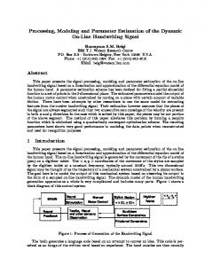
FIG. 4.

Mode Shapes for Two-Dimensional Bridge Model

TABLE 2.

typically observed as a reduction in effective axial or bending rigidities. As formulated here, any inaccuracies in member length will be reflected as modeling error. Material modulus of elasticity is also assumed to be a constant value equal to 29,000 ksi (200,000 MPa). Footing stiffness values are computed assuming a 3-m square footing that is 1 m thick and resting on glacial till. The analytically computed footing stiffness is used as the ‘‘initial’’ guess in parameter estimation. These analytical values, calculated from equations given by Lambe and Whitman (1969) for the diagonal terms and Beredugo and Novak (1972) for the off-diagonal term, K H␪, are analytically calculated ‘‘initial’’ and ‘‘true’’ values for the two scenarios listed in Table 1. Effective soil mass is ignored for this example. Fig. 4 shows the first four modes of vibration using the calculated ‘‘initial’’ values from the software package ANSYS. The joint stiffnesses at nodes 2 and 5 are calculated from the method outlined in the previous sections. The limits for K ␾ are zero for pinned and ⬁ for rigid connection. In this example, the joints are assumed to be partially restrained. Note that the Table 2 value used for K ␾ is empirical and dependent on the connection and structure. If real test data were used, the true values would not be required, and the initial values would not need to be very accurate, as the parameter estimation process would adjust them to more realistically reflect the actual masses and stiffness.

Bridge Example with PRF Elements and SSS Elements in Two Dimensions Number of Iterations

Case number (1)

Measured frequency (2)

Mode shape measured at DOF (3)

Number of measurementsa (4)

Unknown parameter (PU) (5)

1 2 3 4 5 6 7 8 9 10

1–4 1–4 1–4 1–4 1–4 1–3 1–3 1–3 1–2 1

5–9 and 15–20 5–9 and 15–20 5–9 and 15–20 All translational All translational All translational 1–14 15–20 15–20 15–20

44 44 44 48 48 36 42 18 12 6

All 34 Deck and 2(KPRF) 2(Ksss and Msss) Deck and 2(KPRF) 2(KSSS and MSSS) Deck and 2(KPRF) Deck 2(KSSS and MSSS) 2KSSS 2MSSS

a

Number Rank of of PU ST S (7) (6) 34 16 18 16 18 16 10 18 12 6

34 16 18 16 18 16 10 18 10 6

Scenario 1 (8)

Scenario 2 (9)

III-conditioned 5 3 4 18 4 2 3 Singular 2

III-conditioned 8 3 5 III-conditioned 5 2 3 Singular 2

Number of measurements in column (4) equals number of frequencies in column (2) multiplied by number of DOF in (3). For example, in case 1, there are 4 measured frequencies and 11 measured DOF resulting in a total of 44 measurements. 1052 / JOURNAL OF STRUCTURAL ENGINEERING / SEPTEMBER 1999

In this example, the measured natural frequencies and mode shapes of the bridge are simulated by evaluating the eigenvalue problem with the true values of the structural stiffness parameters. Programs such as PCModal, ModalCIS, and XModal are readily available to extract frequencies and mode shapes for frequency response functions at measured DOF. Different combinations of mode shape measurements and applied frequencies are considered. A required but not necessarily sufficient condition for convergence is to have at least as many measurements as unknown parameters. The cost of the NDT is dependent on the number of measurements; thus, the fewer measurements made, the more economical the test. Simulated measured modal data are used to examine the capabilities and limitations of the proposed method for estimation of geometric parameters of frame elements, PRF elements, and SSS elements. Geometric parameters of each frame element are axial rigidity (EA) and bending rigidity (EI ). The parameters of each PRF element are EA, EI, and the torsional rigidity K ␾ at the top of each column. The parameters of each SSS element are K HH, K HV, K H␪, KVV, KV␪, K ␪␪, MHH, MVV, and M␪␪. Two damage scenarios are presented here to examine convergence characteristics when the scaling of the initial values with respect to the true values is not constant. There are two types of parameters: known and unknown. For the known parameters, the initial and true values are the same, and they are not allowed to vary during the estimation process. The initial and true values of the unknown parameters are different, and these parameters are updated through the parameter estimation process. When field NDT data sets are available, the estimation is performed with the best guesses as the ‘‘initial values,’’ and the ‘‘measured’’ frequencies and sparse mode shape values are used to seek the ‘‘true values.’’ However, in this paper, NDT data sets are not available, and the mode shapes and frequencies are simulated using the assumed ‘‘true’’ values with the ratios given in Table 1. Ten cases for parameter estimation of the bridge model, shown in Fig. 4, are simulated, and the results for each damage scenario are shown in Table 2. All cases have the same initial values or best guesses. For cases where some parameters are known, the parameters are assigned true values that are assumed to be accurate. In the cases when geometric parameter estimation converged, the ‘‘true’’ values of the parameters were identified with no bias within a specified tolerance limit. The purpose of these simulations is to find a stable combination of measured frequencies and associated sparse mode shape values to successfully determine a useful set of unknown parameters. Column 1 of Table 2 is the case number for the simulated scenario; column 2 is the list of measured frequencies used in parameter estimation; column 3 is the measured mode shape values (corresponding to the frequencies in column 2) at the selected DOF; column 5 contains the unknown parameters to be estimated. As presented in the section on parameter estimation, the number of measurements in column 4 must be greater than or equal to the number of unknown parameters in column 6 as a minimum requirement for successful parameter estimation. Parameters in column 5 are identifiable parameters if the rank of the system of equations in column 7 is equal to the number of unknown parameters in column 6. Columns 8 and 9 indicate the number of iterations used for convergence to the ‘‘true’’ values of the parameters within a user-specified tolerance for damage scenarios 1 and 2, respectively. If a rank deficiency is indicated by column 7, it is reflected in column 8 or 9 as ‘‘Singular.’’ If the rank is sufficient and convergence is not achieved due to ill-conditioning of the system of equations, it is indicated as ‘‘Ill-conditioned.’’ The goal is to find a small subset of measurements for a potential NDT that leads

to successful parameter estimates with a well-conditioned system of equations. Accuracy of the parameter estimates from an ill-conditioned system of equations is highly dependent on uncertainties in the measurements. Singularity occurs when there is a rank deficiency (i.e., not enough information to estimate all unknown parameters). The cases shown here are intended to show the range in solution possibilities using a maximum of four modes. In all of the runs, the final estimate obtained in the example is a true convergence and corresponds to a global minimum of the objective function. Cases 1–10 are simulations of various combinations of frequencies and mode shape values for potential use of NDT data for parameter estimation. The first three cases concentrate on using a subset of measurements, at the top and the base of the piers, and the first four modes of vibration, which are shown in Fig. 4. Case 1 had all parameters unknown but did not converge due to ill-conditioning. Case 2 dealt with the deck and both PRF elements as unknown and converged on the ‘‘true values’’ of the unknown parameters. Case 3 dealt with the stiffness and mass of the foundation and converged in three iterations in both scenarios. The next two cases used the same four modes of vibration but measurement at all translational DOF. The deck and both PRF elements were considered unknown in case 4, which converged within a small number of iterations. In case 5, the stiffness and mass of the foundation were unknown and converged in 18 iterations for scenario 1, while it was ill-conditioned in scenario 2. The high number of iterations required for convergence in scenario 1 shows that this was not an ideal measurement combination for parameter estimation. Therefore, the ill-conditioning of scenario 2 reinforces this observation. Case 6 used the same measured DOF but only the first three modes of vibration. With 36 measurements, the parameters of the deck and columns were successfully estimated. In case 7, all DOF of the deck are measured for the first three frequencies. The parameters of the deck were identified correctly with only two iterations for both scenarios. The last three cases concentrate on estimation of the foundation parameters. There are two footings each with six unknown stiffness parameters and three unknown mass parameters each, giving a total of 18 unknown stiffness and mass parameters. Using the first three frequencies and the three mode shape values at the base of each column in case 8, all parameters are successfully estimated in three iterations for both scenarios. In case 9, the first two frequencies are measured and modal values at the same DOF are measured. Due to a rank deficiency in the system of equations (singularity), the parameters were not found. In case 10, measuring the first frequency at the same DOF as case 9, the mass parameters of both foundations were accurately estimated in two iterations for both scenarios. In cases 8, 9, and 10, the number of the unknown parameters is equal to the number of measurements. Both occurrences of ill-conditioning and singularities in the minimization process represent important information regarding the error function and both the number and locations of the measurements and unknown parameters. The meaning of the ‘‘singularities,’’ in the context of parameter estimation, describes a situation where at least one of the parameters is not observable by the measurements. ‘‘Ill-conditioned’’ indicates that at least one parameter is barely observable by the measurements. In both singular and ill-conditioned cases, it is advisable to change the measured modes of vibration. The objective is to significantly excite every structural member with an unknown parameter at least once and observe the response by strategic selection of sensor locations. The cases used as examples in Table 2 were intended to show the types of problems typically encountered in parameter estimation. JOURNAL OF STRUCTURAL ENGINEERING / SEPTEMBER 1999 / 1053

The two damage scenarios presented parameter values with a mix of initial guess to true value ratios of 50 to 200% and successfully converged on the true values. It is important to note that the observations made for this example are specific to this error function and solution algorithm and may not apply to other error functions or examples. CONCLUSIONS The ‘‘modal stiffness-based error function’’ was developed for use in parameter estimation. Using this error function, the unknown stiffness and mass parameters of a bridge model at the element level were successfully estimated with no bias. This example included parameter estimation using complete or incomplete sets of modal test data. It was shown that algorithm convergence was affected by selection of the natural frequencies in addition to selection of the number and location of modal measurements. Parameter estimation was used with two superelements to capture complicated foundation system and connection behavior, thereby improving the accuracy of the FEM. The SSS element models the foundation (deep or shallow) by coupling DOF in a full stiffness matrix. The PRF element models partially restrained joints with the addition of an internal rotational DOF with a rotational resistance of K ␾. Both elements were used successfully in a 2D bridge example with simulated modal data. When the parameter estimation routine converged, the parameters associated with all unknown bridge elements were correctly estimated. For convergence of parameter estimation (which is the solution of the inverse problems), the measured modes at the selected DOF must fully excite and observe the changes in the unknown parameters. As more bridges require maintenance and rehabilitation, there is an emerging need to understand the current state of these bridges. Many have unknown substructures, and tools such as parameter estimation can lead to improving our understanding of the complicated foundation system and connection behavior. An essential step described in this paper is the evaluation of algorithm performance and experiment design. ACKNOWLEDGMENTS The research presented in this paper has been partially supported by NSF grant numbers CMS-9622067 and CMS-9622515. The writers are grateful for the contributions made by Inna Gornshteyn, who graduated from Tufts University with an MS degree in 1992, in the development of modal parameter estimation. In addition, the writers are grateful to Behnam Arya, a doctoral student at Tufts University who helped to enhance our parameter estimation software.

APPENDIX I.

REFERENCES

Aristizabal-Ochoa, J. D. (1997). ‘‘First- and second-order stiffness matrices and load vector of beam-columns with semirigid connections.’’ J. Struct. Engrg., ASCE, 123(5), 669–678. Arya, B., Santini, E. M., and Sanayei, M. (1998). ‘‘Impact of finite element modeling error on model updating.’’ Proc., 2nd World Congr. on Struct. Control, Wiley, New York, 2269–2278. Azizinamini, A., Bradburn, J. H., and Radziminski, J. B. (1987). ‘‘Initial stiffness of semi-rigid steel beam-to-column connections.’’ J. Constr. Steel Res., 8, 71–90. Beck, J. L., and Jennings, P. C. (1980). ‘‘Structural identification using linear models and earthquake records.’’ Earthquake Engrg. and Struct. Dyn., 8(2), 145–160. Beck, J. L., and Katafygiotis, L. S. (1998). ‘‘Updating models and their uncertainties. I: Bayesian statistical framework.’’ J. Engrg. Mech., ASCE, 124(4), 455–461. Beredugo, Y. O., and Novak, M. (1972). ‘‘Coupled horizontal and rota1054 / JOURNAL OF STRUCTURAL ENGINEERING / SEPTEMBER 1999

tional vibration of embedded footings.’’ Can. Geotech. J., Ottawa, 9(4), 477–497. Chan, S. L. (1994). ‘‘Vibration and modal analysis of steel frames with semi-rigid connections.’’ Engrg. Struct., 16(1), 25–31. Davison, J. B., Kirby, P. A., and Nethercot, D. A. (1987). ‘‘Rotational stiffness characteristics of steel beam-to-column connections.’’ J. Constr. Steel Res., 8, 17–54. Doebling, S. W., Farrar, C. R., Prime, M. B., and Shevitz, D. W. (1996). ‘‘Damage identification and health monitoring of structural and mechanical systems from changes in their vibration characteristics: A literature review.’’ Rep. No. LA-13-70-MS, Los Alamos National Laboratory, Los Alamos, N.M. Ewins, D. J. (1984). Modal testing: Theory and practice, Research Studies Press Ltd., Letchworth, U.K. Gangadharan, S. N., Nikolaidis, E., and Haftka, R. T. (1991). ‘‘Probabilistic system identification of two flexible joint models.’’ AIAA J., 29(8), 1319–1326. Ghanem, R., and Shinozuka, M. (1995). ‘‘Structural-system identification. I: Theory.’’ J. Engrg. Mech., ASCE, 121(2), 255–264. Gornshteyn, I. (1992). ‘‘Parameter identification of structures using selected modal measurements,’’ MS thesis no. 4340, Tufts University, Medford, Mass. Gunes, B., Arya, B., Wadia-Fascetti, S., and Sanayei, M. (1999). ‘‘Practical issues in the application of structural identification.’’ Computational mech. in struct. engrg.: Recent devel., F. Cheng and Y. Gu, eds., Elsevier Science, Oxford, U.K., 193–206. Hart, G. C., and Yao, J. T. P. (1977). ‘‘System identification in structural dynamics.’’ J. Engrg. Mech., ASCE, 103(6), 1089–1104. Hjelmstad, K. D., Banan, M. R., and Banan, M. R. (1995). ‘‘Time-domain parameter estimation algorithm for structures. I: Computational aspects.’’ J. Engrg. Mech., ASCE, 121(3), 424–434. Holzer, S. M. (1985). Computer analysis of structures: Matrix structural analysis structured programming. Elsevier Science, New York. Ibrahim, S. R. (1983). ‘‘Computations of normal modes from identified complex parameters.’’ AIAA J., 21(3), 446–451. Kim, J.-T., and Stubbs, N. (1995). ‘‘Model-uncertainty impact and damage-detection accuracy in plate girder.’’ J. Struct. Engrg., ASCE, 121(10), 1409–1417. Kishi, N., and Chen, W. F. (1986). ‘‘Data base of steel beam-to-column connections,’’ Tech. Rep., Vols. I and II, School of Engrg., Purdue University, West Lafayette, Ind. Lambe, T. W., and Whitman, R. V. (1969). Soil mechanics. Massachusetts Institute of Technology, Cambridge, Mass., 231–232. Liu, S.-C., and Yao, J. T. P. (1978). ‘‘Structural identification concept.’’ J. Struct. Engrg., ASCE, 104(12), 1845–1858. Maxwell, J. C., and Briaud, J.-L. (1994). ‘‘53 WAK tests on spread footings.’’ Vertical and Horizontal Deformations of Found. and Embankments, Vol. 1, Proc. of Settlement ’94, Geotech. Spec. Publ. No. 40, Albert T. Yeung and Guy Y. Felio, eds., ASCE, New York, 143–152. McClain, J. (1996). ‘‘Parameter estimation for large scale structures,’’ MS thesis no. 4939, Tufts University, Medford, Mass. Mottershead, J. E., and Friswell, M. I. (1993). ‘‘Model updating in structural dynamics: A survey.’’ J. Sound and Vibration, 167(2), 347–375. Olson, L. D., and Wright, C. C. (1989). ‘‘Nondestructive testing of deep foundations with sonic methods.’’ Found. Engrg. Current Principles and Pract., ASCE, New York, 1173–1183. Robson, B. N., Frangopol, D. M., and Goble, G. G. (1992). ‘‘Improving correlation between experimental bridge strains and analytical models through optimization.’’ Proc., 3rd Int. Workshop on Bridge Rehabilitation, Technical University Darmstadt and the University of Michigan, Darmstadt, Germany, 559–570. Sanayei, M. (1998). ‘‘PARIS: PARameter Identification System,’’ Reference manual, Tufts University, Medford, Mass. Sanayei, M., Doebling, S. W., Farrar, C. R., and Wadia-Fascetti, S. (1998a). ‘‘Challenges in parameter estimation for condition assessment of structures.’’ Proc., Struct. Engrs. World Congr., Elsevier Science, New York, T216–5. Sanayei, M., Imbaro, G., McClain, J. A. S., and Brown, L. C. (1997). ‘‘Parameter estimation of structures using NDT data: Strains or displacements.’’ J. Struct. Engrg., ASCE, 123(6), 792–798. Sanayei, M., and Onipede, O. (1991). ‘‘Damage assessment of structures using static test data.’’ AIAA J., 29(7), 1174–1179. Sanayei, M., Onipede, O., and Babu, S. R. (1992). ‘‘Selection of noisy measurement locations for error reduction in static parameter identification.’’ AIAA J., 30(9), 2299–2309. Sanayei, M., and Saletnik, M. J. (1996a). ‘‘Parameter estimation of structures from static strain measurements; Part I: Formulation.’’ J. Struct. Engrg., ASCE, 122(5), 555–562.

Sanayei, M., and Saletnik, M. J. (1996b). ‘‘Parameter estimation of structures from static strain measurements; Part II: Error sensitivity analysis.’’ J. Struct. Engrg., ASCE, 122(5), 563–572. Sanayei, M., Wadia-Fascetti, S., McClain, J. A. S., Gornshteyn, I., and Santini, E. M. (1998b). ‘‘Structural parameter estimation using modal responses and incorporating boundary conditions.’’ Proc., Struct. Engrs. World Congr., San Francisco, Calif., T216–4.

Shinozuka, M., and Ghanem, R. (1995). ‘‘Structural system identification. II: Experimental verification.’’ J. Engrg. Mech., ASCE, 121(2), 265–273. Topole, K. G., and Stubbs, N. (1995). ‘‘Non-destructive damage evaluation of a structure for limited modal parameters.’’ Earthquake Engrg. and Struct. Dyn., 24, 1427–1436. Veletsos, A. S., and Wei, Y. T. (1971). ‘‘Lateral and rocking vibrations of footings.’’ J. Soil Mech. and Found. Div., ASCE, 97(7), 1227–1248.

JOURNAL OF STRUCTURAL ENGINEERING / SEPTEMBER 1999 / 1055