INCREMENTAL INDUCTIVE LEARNING ALGORITHM IN THE FRAMEWORK OF ROUGH SET THEORY AND ITS APPLICATION Won-Chul BANG a,
Zeungnam BIEN b
Dept. of Electrical Engineering, KAIST 373-1 Kusong-dong, Yusong-gu, Taejon 305-701, Korea a. Tel:+82-42-869-8019 Fax:+82-42-869-8751 E-mail:
[email protected] b. Tel:+82-42-869-3419 Fax:+82-42-869-8751 E-mail:
[email protected] Abstracts In this paper we will discuss a type of inductive learning called learning from examples, whose task is to induce general descriptions of concepts from specific instances of these concepts. In many real life situations, however, new instances can be added to the set of instances. It is first proposed within the framework of rough set theory, for such cases, an algorithm to find minimal set of rules for decision tables without recalculation for overall set of instances. The method of learning presented here is based on a rough set concept proposed by Pawlak[2][11]. It is shown an algorithm to find minimal set of rules using reduct change theorems giving criteria for minimum recalculation with an illustrative example. Finally, the proposed learning algorithm is applied to fuzzy system to learn sampled I/O data. Keywords: Incremental Inductive Learning, Rough Set Theory, Fuzzy Learning
1.
Introduction
The subject of machine learning has received considerable attention in recent decades. Inductive learning (learning from examples) is perhaps the oldest and best-understood problem in artificial intelligence[4]. Many existing expert systems were built by manually encoding the knowledge of human experts. Encoding processes as such can be very time consuming as they require close collaboration between computer professionals and experts of the subjects domain. To design expert system in this way is rather inefficient particularly because the same tedious task has to be performed for each specialized application. A better alternative of designing an expert system would be to construct and inductive algorithm that can, from a carefully chosen sample of expert decisions, infer and refine decision rules automatically independent of the subject of interest. The papers [5][6][7][10] describe some of the more recent research efforts made in this area. Quinlan[1] suggested an inductive algorithm based on the statistical theory of information originally proposed by Shannon. The entropy function is used as a measure of uncertainty in the classification of objects characterized by attributes and attribute values. On the other hand, Pawlak[2] showed that the principles of inductive learning can be formulated precisely and in a unified way within the framework of rough set theory. The set of instances, which is used for training set of learning, is usually constant and unchanged during the learning process. In many real life situations however this is not the case and new instances can be
added to the set of instances. Our main objective in this paper is to find an algorithm for inductive learning without any recalculation for overall instances when a new instance is added within the framework of rough set theory assuming that the minimized decision rules for the original decision table is already given. In section 2, the preliminaries for rough set theory are reviewed, especially for the previous algorithm for minimizing of decision tables. In section 3, inductive learning concept in view of rough set theory is given. Based on this scheme, an algorithm for learning from examples when a new instance is added to the examples in section 4 and finally, fuzzy learning system is introduced as an application. 2.
Mathematical Preliminaries
In this section, in order to deal with decision tables mathematically, mathematical backgrounds on rough set theory and related definition are reviewed. In addition, the existing minimization method of decision table is followed up to catch an idea to lead the proposed algorithm. 2.1 Formal Definitions and Semantics of Decision Logic[8] Decision tables can be defined in terms of KR(Knowledge Representation)-systems as follows. Let K = (U, A) be a KR-system and let C, D Ι A be two subsets of attributes, called condition and decision attributes respectively. KR-system with distinguished condition and decision attributes will be called a decision table and will be denoted
T=(U,A,C,D), or in short CD-decision table. Equivalence classes of the relations IND(C) and IND(D) will be called condition and decision classes, respectively. With every x Ι U we associate a function dx:A′ V, such that dx(a) = a(x), for every a Ι C Ε D; the function dx will be called a decision rule in T, and x will be referred as a label of the decision rule dx. Expressions of the form (a, v), or in short av, called atomic formula, are formulas of the DL(Decision Logic)-language for any a Ι A and vΙVa. If φ and ϕ are formulas of the DL-language, then so are ~φ, (φ Υ ϕ), (φ Υ ϕ), (φ ′ ϕ), and (φ ♦ ϕ). Formulas are meant to be used as descriptions of objects of the universe. Atomic formula (a, v) is interpreted as a description of all objects having value v for attribute a. Compound formulas are interpreted in the usual way. In order to express this problem more exactly, we define Tarski¡s style semantics of the decision logic language. An object x Ι U satisfies a formula φ in S = (U, A), denoted x |=s φ or in short x |= φ, if S is understood. If φ is a formula the set |φ|s defined as follows |φ|s = {x Ι U | x |=s φ} will be called the meaning of the formula φ in S. Formula of the form (a1, v1) Υ (a2, v2) Υ ¡ Υ (an, vn), where vi Ι Vai, P = {a1, a2, ¡ , an}, and P Ι A, will be called a P-basic formula or in short Pformula. A-basic formula will be called basic formulas. Any implication φ ′ ϕ will be called a decision rule in the KR-language; φ and ϕ are referred to as the predecessor and the successor of φ ′ ϕ respectively. If a decision rule φ ′ ϕ is true in S, it is said that the decision rule is consistent in S. If φ ′ ϕ is a decision rule and φ and ϕ are P-basic and P-basic formulas respectively, then decision rule φ ′ ϕ will be called a PQ-basic decision rule, (in short PQrule), or basic rule when PQ is known. Any finite set of basic decision rules will be called a basic decision algorithm. If all decision rules in a basic decision algorithm are PQ-decision rules, then the algorithm is said PQ-decision algorithm, or in short PQ-algorithm, and will be denoted by (P, Q). The PQ-algorithm is consistent in S, iff its decision rules are consistent in S. 2.2 Minimization of Decision Tables The approach to table minimization presented in [8] consists of the following steps: Step 1) Reduction of the Algorithm: Computation
of reduct of condition attributes which is equivalent to elimination of some column from the decision table. Step 2) Reduction of Decision Rules: Elimination of superfluous values of attributes. Step 3) Minimization of the Decision Algorithm: Elimination of superfluous decision rules. Now each step is introduced in detail one by one. Let (P, Q) be a consistent algorithm and suppose that a Ι P and R Ι P. Step 1) Reduction of the Algorithm: An attribute a Ι P is called dispensable in the algorithm (P, Q) if the algorithm (P-{a}, Q) is consistent; otherwise a is indispensable in (P, Q). The algorithm (P, Q) is called independent if all aΙP are indispensable in (P, Q). The subset of attributes RΙ P is called a reduct of the algorithm (P,Q) if (R,Q) is independent and consistent. A basic decision algorithm is said to be reduced if every rule in the algorithm is reduced. Step 2) Reduction of Decision Rules Let φ ′ ϕ be a PQ-rule. An attribute a Ι P is called dispensable in the rule φ ′ ϕ if |=s φ ′ ϕ implies |=s φ/(P-{a}) ′ ϕ; otherwise a is indispensable in φ ′ ϕ. The PQ-rule φ′ ϕ is called independent if all aΙP are indispensable in φ ′ ϕ. The subset of attributes RΙ P is called a reduct of the PQ-rule φ ′ ϕ if φ/R ′ ϕ is independent and |=s φ ′ ϕ implies | =s φ/R ′ ϕ. A decision rule φ/R ′ ϕ is said to be reduced if R is a reduct of the PQ-ruleφ ′ ϕ. Step 3) Minimization of the Decision Algorithm The set of all rules in A having the same successor ϕ is denoted Aϕ, and Pϕ is the set of all predecessors of decision rules belonging to Aϕ. A decision rule φ′ ϕ in A is called dispensable in A if |=s Υ Pϕ ♦ {Pϕ-{φ}}, where Υ Pϕ denotes disjunction of all formulas in Pϕ; otherwise φ ′ ϕ is indispensable in A. The set of rules Aϕ is called independent if all decision rules in Aϕ are indispensable in Aϕ. The subset A¡ of decision rules of Aϕ is called a reduct of Aϕ if all decision rules in A¡ are independent and |=s Υ Pϕ ♦ Pϕ¡. A set of decision rules Aϕ is said to be reduced if reduct of Aϕ is Aϕ itself. A basic algorithm A is said to be minimal if every decision rule in A is reduced and for every decision rule φ ′ ϕ in A, Aϕis reduced. 3.
Inductive Learning
3.1 Learning from Examples Assume that there are two agents: a ¡knower¡ and a ¡learner¡. Suppose that the knower has knowledge about certain universe of discourse U, that is, he is
able to classify elements of the universe U, and classes of the knower¡s classification from concepts to be learned by the learner. Moreover, it is assumed that the knower has complete knowledge about the universe U and the universe U is closed that is nothing else besides U exists. This assumption is called the closed world assumption(CWA)[8]. Task of a learner is to learn knower¡s knowledge. Now the problem whether always the learner¡s knowledge can match the knower¡s knowledge or whether the knower¡s knowledge (attributes) depends on learner¡s knowledge (attributes). As a consequence the degree of dependency between the set of knower¡s and learner¡s attribute, can be viewed as a numerical measure of how exactly the knower¡s knowledge can be learned. To describe this concept, Pawlak[2] defined the quality of learning as follows: k = γ B (C ) =
cardPOS B (C ) cardU
which is the same quantity with the degree of dependency. This number expresses what percentage of knower¡s knowledge can be learned by the learner. 3.2 Dynamic Learning The learning under closed world assumption is viewed as a static learning[2]. The classification rules learned from training examples can be assumed as the background knowledge of the learner. The question arises whether the background knowledge can be used to classify correctly new object not occurring in training examples which occurs under open world assumption(OWA)[8]. Classification of new objects based on background knowledge previously acquired from training examples is considered dynamic learning[2]. Pawlak categorized the possibilities when a new instance is added as follows: 1) the new instance confirms actual knowledge 2) the new instance contradicts actual knowledge 3) the new instance is completely new case. If the training set is in a certain sense complete, i.e., the decision table is consistent if provides the highest quality of learning and the learners knowledge cannot be improved by means of new instances. If however the training set is inconsistent, every new confirming instance increases learner¡s knowledge and any new borderline instance decreases his knowledge. 4.
Proposed Algorithm
4.1 Refinement of Categorization for New Instances Observing carefully the steps to minimize decision tables in the previous section gives an idea to make
an update law of the minimized decision rules when a new instance is added. While Pawlak[2][8] considered three possibilities when adding a new instance to the universe as introduced in the last section, we propose four possibilities. Before going ahead, it is required to define several concepts. Definition 1. Completely contradict: A new instance x is said to be completely contradict if x contradicts the given minimized decision rules and there exists a y Ι U such that φx ♦ φy, where x is φx ′ ϕx and y is φy ′ ϕy. z Definition 2. Partially contradict: A new instance x is said to be partially contradict if x contradicts the given minimized decision rules and it doesn¡t completely contradict the given decision rules. z Now we can suggest categorize the cases when a new instance to the universe as follows: 1) the new instance confirms actual knowledge 2) the new instance completely contradicts actual knowledge 3) the new instance partially contradicts actual knowledge 4) the new instance is completely new case. 4.2 Criteria to Change Reducts In this paper, we only consider the case when a partially contradict instance is added to the universe. The minimization method of decision tables find a Q-reduct of P, and then find reducts for each rule, that is, eliminate superfluous values of attributes, and finally find a reduct for the generated rules in the previous step, i.e., eliminate superfluous decision rules. Now assume that the minimized decision rules for a decision table and all kinds of reduct corresponded are given before a new instance is added. Likewise the minimization steps, now when a new instance is added, the proposed algorithm first checks if the Qreduct of P should be changed(step 1). If so, find rules for which the reduct for each rule should be updated and recalculate them(step 2). Finally, eliminate superfluous decision rules for newly created decision rules(step 3). In order to check whether the Q-reduct of P should be changed or not, we have a criterion to decide it. The theorem 1[12] gives us such a criterion. Theorem 1. Suppose S = (U, A) is a KR-system
and a new instance x is added to U with a basic decision rule φx ′ ϕx which partially contradicts the acquired knowledge. Then the reduct of the PQ-basic algorithm, RED(P, Q) changes if and only if there z exists a y Ι U such that y |=s φx / RED(P, Q).
4, 5, 6, 7}, A = P Ε Q, P = {a, b, c, d}, and Q = {e}. The decision table is given in the table 1. Table 1. A decision table U a b c d e 1 1 0 0 1 1 2 1 0 0 0 1 3 0 0 0 0 0 4 1 1 0 1 0 5 1 1 0 2 2 6 2 2 0 2 2 7 2 2 2 2 2
In order to find the rule set which the reduct for each rule should be updated, we use the following. Remark 1. Suppose S = (U, A) is a KR-system and a new instance x is added to U with a basic decision rule φx ′ ϕx which partially contradicts the acquired knowledge. Then, we intuitively insist that, for each i Ι U¡(= U Ε{x}), the reduct of decision rule φi ′ ϕi, RED(φx ′ ϕx) does not changes if and only if φi/RED(φi ′ ϕi) = φx/RED(φi ′ ϕi) implies φi ′ ϕi. From the above consideration we can make a set of label of which rules in the original minimized set of rules is contradicted by x. Let us denote such a label set be cx. The overall flowchart of proposed algorithm is given in the figure 1.
The minimized decision rules and a Q-reduct of P can be found from the steps in the previous section as follows: a1b0 ′ e1 a0 ′ e0 b1d1 ′ e0 d2 ′ e2 and RED(P, Q) = {a, b, d}.
New instance x with basic rule φ x′ ϕ x x is new or completely contradict
Suppose a new instance x U a b c D e x 0 1 2 1 1
x confirms Nothing Changed
End
Find minimized rules for all instances
End
Which case? x is partially contradicts
For Step 1
Same RED(P,Q)?
N
Y Find cx For Step 2
Find new RED(φi′ ϕi) for i Ι cx
is added which partially contradicts the previously acquired knowledge. By the theorem 1, we can know RED(P, Q) doesn¡t change since no y Ι U and y |=s φx / RED(P, Q). Moreover, the remark 1 yields the label set and corresponding reduct for each rule: cx = {3, 4} RED(φ3 ′ ϕ3) = {a, b}, {a, d} RED(φ4 ′ ϕ4) = {a, b, d} RED(φx ′ ϕx) = {a, b}, {a, d}
Find new RED(φx′ ϕx)
For Step 3
Reduce the set of rules for each class of cx Reduce Aϕx
For e0, a0b0 ′ e0 or a0d0 ′ e0 a1b1c0 ′ e0,
3: 4:
we can choose a0b0 ′ e0, a1b1c0 ′ e0
End
On the other hand, for Aϕx, i.e., e1, Fig. 1. Proposed inductive learning algorithm when a new instance is added
1, 2: x:
a1b0 ′ e1 a0b1 ′ e1 or a1d0 ′ e1,
4.3 An Illustrative Example we can choose Here is a KR-system S = (U, A) where U = {1, 2, 3,
(1)
a1b0 ′ e1, a0b1 ′ e1 (2)
A new concept, indiscernibility between attribute values is defined as follows, by which we solve the above problem.
Therefore the total minimized decision rules are a0b0 ′ e0 a1b1c0 ′ e0 a1b0 ′ e1 a0b1 ′ e1 d2 ′ e2
from (1) from (2) ¡ no change
which is identical to the result of recalculation for overall set of instances. 5.
Definition 3. Indiscernibility between attribute values: Suppose we have found a set of minimized rules for a given decision table. For two rules with the same consequent, say, φ1 ′ ϕ which φ2 ′ ϕ, the two attribute values va1 and va2 of attribute a are called indiscernible iff φ1 has va1, φ2 has va2 and all the other attribute values between φ1 and φ2 are the same. z
An Application to Fuzzy Learning
One of the possible approaches to design a controller for a very complex plant controlled by human is to design a controller emulating the control actions of the human by using sampled I/O data from the actions of the human. When there is no mathematical model or the mathematical model is strongly nonlinear, it is advantageous to design a fuzzy controller. Wang and Mendel[9] proposed a general method to generate fuzzy rules by learning form examples. It proved to be capable of approximating any real continuous function on a compact set to arbitrary accuracy. However, it does not determine the domain intervals and the shape of each membership function, which have a great effect on the performance of a fuzzy system. Proposed incremental inductive learning algorithm can effectively deal with the large amount of I/O data. However, there is a problem before it is applied to fuzzy learning. It will be solved by the new concept of indiscernibility between attribute values and then, it will be explained how to generate fuzzy rules. 5.1 Clustering Attribute Values When the attribute values are real, rough set approach cannot consider whether one is bigger than another. We hope that we can still classify although the attribute values are real. In view of rough set approach, an attribute value, say 4.8, doesn¡t have any meaning to another attribute value, say 5.2, just as an attribute value ¡red¡ doesn¡t have it to another attribute value ¡blue¡. That is, the magnitude of numbers cannot be considered. From the above consideration, in order to cluster the attribute values in the continuous domain, it is reasonable to minimize the number of rules minimized by rough set technique such that the new set of minimized rules with the new attribute values does not conflict to the sampled I/O data pairs by clustering each set of attribute values for all attributes and redefining each set of attribute values with the clusters.
The above definition is intuitively understood and reasonable to minimize the number of rules. For each attribute, any two attribute values which are indiscernible can be clustered. 5.2 Generating Fuzzy Rules Once we find the minimal number of rules by clustering the attribute values, we can assign linguistic variables to every attribute and make their term sets with clusters in each attribute. The overall procedures can be summarized as follows. Step 1. Find the set of minimized rules for given decision table. Step 2. Divide the output space into fuzzy regions to make fuzzy linguistic variable for output. Step 3. Cluster the attribute values in the sense of indiscernibility between attribute values. Step 4. Divide the input space using clusters acquired in step 3. Step 5. Create a fuzzy rule base with the fuzzy term sets. With this procedure, we can make a fuzzy rule base from the given sampled I/O data. Next, the proposed incremental inductive learning algorithm is applied to this fuzzy learning system for online control, diagnosis, etc. 6.
Concluding Remarks
In this paper, it is shown a type of inductive learning, whose task is to induce general descriptions of concepts from specific instances of these concepts. It is proposed, when a new instance is added to the universe of discourse, an algorithm to find minimal set of rules for decision tables without recalculation for overall set of instances. The main contribution of this paper is to provide an algorithm of inductive learning for additive instances to efficiently increase the total learned knowledge within the framework of rough set theory assuming that the minimized decision rules for the
original decision table is already given. At last, it is shown that the proposed algorithm can be applied to fuzzy learning system. This paper still leaves several further works to make the algorithm perfect for any kinds of new instances. The proposed algorithm does not consider the cases when the new instance is completely new case to the previously acquired knowledge and when it completely contradicts the knowledge. An algorithm to cope with these two cases would be acquired from the mathematical analysis with semantics of decision logic language.
Preferential Attitude in Multi-Criteria Decision Making,¡± Pr oc. I nt. Sy mp. on Met hodol ogi es f or Intelligent Systems or Lecture Notes in Artificial Intelligence, J. Komorowski, et al.(eds.), vol. 689, pp. 642-651, 1993 11. Z. Pawlak, ¡Data Analysis with Rough Set Theory,¡± Pr oc. ofKFIS Fall Conference ¡96, vol. 6, no. 2, pp. 3-19, 1996 12. W.-C. Bang, and Z. Bien, ¡Inductive Learning Algorithm using Rough Set Theory,¡±Proc. of KFIS Fall Conference ¡97, vol. 7, no. 2, pp. 331337, 1997
References
Appendix
1. J. R. Quinlan, ¡Learning Efficient Classification Procedures and Their Application to Chess End Games,¡ Machine Learning: An Artificial Intelligence Approach, R. S. Michalski, et al.(eds.), Morgan Kaufmann Publishers, Inc., 1983 2. Z. Pawlak, ¡On Learning ? A Rough Set Appoach,¡± Pr oc. I n. Symp. on Computation Theory or Lecture Notes in Computer Science, G. Goos, et al.(eds.), vol. 208, pp. 197-227, 1984 3. Z. W. Ras, et al., ¡°Roug-Sets Based Learning System,¡± Pr oc. I n. Symp. on Computation Theory or Lecture Notes in Computer Science, G. Goos, et al.(eds.), vol. 208, pp. 265-275, 1984 4. R. Forsyth, Machine Learning: Applications in Expert Systems and Information Retrieved, John Wiley & Sons, 1986 5. T. Arciszewski, et al., ¡A Methodology of Design Knowledge Acquisition for Use in Learning Expert Systems,¡±Int. J. of Man-Machine Studies, vol. 27, pp. 23-32, 1987 6. R. Yasdi, et al., ¡An Expert System for Conceptual Schema Design: A Machine Learning Approach,¡± Int. J. of Man-Machine Studies, vol. 29, pp. 351376, 1988 7. J. W. Grzymala-Busse, et al., ¡On the Unknown Attribute Values in Learning from Examples,¡± Proc. Int. Symp. on Methodologies for Intelligent Systems or Lecture Notes in Artificial Intelligence, Z. W. Ras, et al.(eds.), vol. 542, pp. 368-377, 1991 8. Z. Pawlak, Rough Sets: Theoretical Aspects and Reasoning about Data, Kluwer Academic Publishers, 1991 9. L. X. Wang and J. M. Mendel, ¡Generating Fuzzy Rules by Learning from Examples,¡±IEEE Trans. Syst., Man, and Cybern., vol. 22, no. 6, pp. 14141427, 1992 10. R. Slowinski, ¡Rough Set Learning of
Proof of theorem 1. Suppose first there does not exist any y Ι U such that y |=s φx/R where R = RED(P, Q). Then a new rule x does not conflict to any previous rules in (R, Q). Hence (R, Q) is consistent in the universe of discourse after adding the new instance, denoted by U¡. By definition of RED(P, Q), RED(P, Q) is indispensable in (R, Q) in U, that is, if any attribute in R is removed then (R, Q) becomes inconsistent in U. This is naturally true whether a new rule x is added to U or not. Hence, RED(P, Q) is indispensable in (R, Q) in U¡ and thus RED(P, Q) is still a reduct in U¡. For reverse implication, let a rule z in the minimized rule set which conflicts to the new rule x. Then, |=s φx ′ ϕ x and φx ♥ ϕ x
(A.1)
where x |=s φx ′ ϕ x and z |=s φz ′ ϕ z. Since φz/R ♦ φz, |=s φx/R ′ φz/R
(A.2)
By assumption, there exists a y Ι U such that y |=s φx/R, i.e., φy/R ♦ φx/R
(A.3)
(A.2) and (A.3) yields |=s φy/R ′ φz/R
(A.4)
And, since y and z are consistent in (R, Q) if |=s φy/R ′ φz/R then φy ♦ φz. This and (A.4) yields φy ♦ φz
(A.5)
From (A.1) and (A.5), φy ♥ φx
(A.6)
In result, from (A.3) and (A.6), φx/R ′ φy/R and φy ♥ φz. Because the new rule x conflicts to y in (R, Q) in U, which implies that R = RED(P, Q) cannot be a reduct of (P, Q) in U¡, the proof is complete. z