Aug 12, 2016 - Email: mateusriva@ usp. br, ponti@ usp. br ... In [6] the authors propose an alternative OPF algorithm which is more ef- .... 2. Predecessor belongs to the same class and is a prototype: we .... examples, 64 features, 14 classes; ... By inspecting the average and standard deviations, it is possible to see.
An incremental linear-time learning algorithm for the Optimum-Path Forest classifier arXiv:1604.03346v1 [cs.LG] 12 Apr 2016
Mateus Riva and Moacir Ponti Instituto de Ciˆencias Matem´aticas e de Computa¸c˜ao, Universidade de S˜ ao Paulo – S˜ao Carlos, SP 13566-590 Brazil Email: mateusriva@ usp. br , ponti@ usp. br
Abstract We present a classification method with linear-time incremental capabilities based on the Optimum-Path Forest (OPF) classifier. The OPF considers instances as nodes of a fully-connected training graph, where the edges’ weights are the distances between two nodes’ feature vectors. Upon this graph, a minimum spanning tree is built, and every edge connecting instances of different classes is removed, with those nodes becoming prototypes or roots of a tree. A new instance is classified by discovering which tree it would conquer. In this paper we describe a new training algorithm with incremental capabilities while keeping the properties of the OPF. New instances can be inserted in the model into one of the existing trees; substitute the prototype of a tree; or split a tree. This incremental method was tested for accuracy and running time against both full retraining using the original OPF and an adaptation of the Differential Image Foresting Transform. The method updates the training model in linear-time, while keeping similar accuracies when compared with the original model, which runs in quadratic-time.
1
Introduction
The optimum-path forest (OPF) classifier [12] is a recently developed classification method that can be used to develop simple, fast, multiclass and parameter independent classifiers. It was shown to be reliable in several applications such as network invasion [14], content based image retrieval [3], image classification [15] and power systems [19], among others. c
2016: This manuscript version is made available under the CC-BY-NC-ND 4.0 license http://creativecommons.org/licenses/by-nc-nd/4.0/
1
1 INTRODUCTION One possible drawback of using the OPF classifier is the training time, which is quadratic on the number of training instances. More specifically, let Z be a training set composed of n examples. The OPF training algorithm then runs in O(n2 ). Some efforts were made to mitigate such running time, by using several OPF classifiers trained with reduced training sets in ensemble learning [17] and fusion using splitted sets using multithread processing [16]. Also, recent work developed strategies to speed-up the training algorithm by taking advantage of data structures and pruning, such as [9, 13]. Considering that the original OPF has no incremental learning capabilities and the current need for methods that can be updated fast, we describe a incremental learning approach for the OPF model. Incremental learning is a machine learning paradigm where the classifier changes and adapts itself to include new examples that emerged after the initial construction of the classifier [6]. As such, an incremental-capable classifier has no strict need for a complete a priori dataset, nor does it need to rebuild itself from the ground up everytime the data domain changes or evolves. It has many practical applications, such as continually adapting to monitor new forms of spam in emails or monetary fraud in bank records; or quickly being able to add a constant stream of input data to itself. Because the OPF is based on the Image Foresting Transform (IFT), a method that was formulated for use only in image pixels [5], and since there is a differential algorithm (DIFT) for it that can update the forests faster than the original IFT [4], it would be a natural algorithm to try in the context of a Incremental OPF. However, the main idea of the DIFT is to include all new pixels as prototypes. In a common scenario for OPF, which deals with feature spaces instead of images, including new patterns in the model as prototypes would progressively convert the model into a 1-Nearest Neighbor classifier. Therefore, we propose a more complex solution, that tries to maintain the connectivity properties of the original OPF method. In this paper, we describe an incremental learning method based on the OPF classifier called the OPF-Incremental (OPFI). Our method is based in graph theory methods which can be used to update minimum spanning trees [2] and optimum paths [1] in order to maintain the graph structure and thus the learning model [8]. We assume there is a initial model trained with the regular OPF, and perform inclusions of new examples appearing over time. Our method displays similar accuracy and distribution of classification results when compared with the original OPF classifier; however, it can add examples to the model in linear time, whereas OPF retraining takes quadratic time. This is an important feature since models should be updated in an efficient way in order to comply with realistic scenarios [7]. Our method c
2016: This manuscript version is made available under the CC-BY-NC-ND 4.0 license http://creativecommons.org/licenses/by-nc-nd/4.0/
2
2 OPF TRAINING ALGORITHM
will be useful everywhere the original OPF was useful, along with fulfilling incremental learning requirements.
2
OPF training algorithm
The optimum-path forest (OPF) classifier [12] interprets the examples (observations) as the nodes (vertices) of a graph. The edges connecting the vertices are defined by some adjacency relation between the examples, weighted by a distance function (e.g. a Minkowski distance). In this model it is expected that training examples from a given class will be connected by a path of nearby examples. Therefore the model that is learned by the algorithm is composed by several trees, each tree containing examples from a given class. The root of each tree is called a prototype. In the next sections the training and classification algorithms of this method are described.
2.1
Training algorithm
The training stage consists in finding prototypes examples in the training set, and determining those examples that will be rooted at them forming trees. Optimum paths are computed from the prototypes to each training example so that each prototype is the root of an optimum-path tree (OPT). The labels of these examples are the same of their root, i.e., all examples in a OPT are from a given class, although each class can have multiple OPTs. In Figure 1 (a)-(c), a simple example is shown to illustrate the training algorithm. First, the algorithm computes a minimum-spanning tree (MST) on a complete graph that is formed by all training examples. Then, since the true labels of the training data are known, key examples (called prototypes) are identified by selecting the vertexes that connect examples from different classes. Each prototype is considered the root of an OPT. Let Z be composed of all n examples (nodes in the sense of a graph) in the training set. Then S is the set of prototypes such that S ⊂ Z. Let also z be an example, i.e., a feature vector with d features, so that z ∈ Rd . The labels of the prototypes are propagated to the other nodes. Therefore, each class may be represented by one or more optimum-path tree. As a result, an optimum-path P ∗ (z) is assigned from S to each node z, yielding the optimum-path forest P . Note that P ∗ (z) = nil when z ∈ S. Along with the optimum-path function, the training algorithm also computes for each node z: the minimum cost on the training set T (z) of P ∗ (z); the class label L(z); and the predecessor of the node, P (z). After this step,
c
2016: This manuscript version is made available under the CC-BY-NC-ND 4.0 license http://creativecommons.org/licenses/by-nc-nd/4.0/
3
2 OPF TRAINING ALGORITHM
the optimum-path forest is available to classify new observations. The Algorithm 1 contains all steps for obtaining the OPF model. It is important to note that there are enhanced versions of this algorithm. Some deal with large datasets, while others can reduce the training error by exchanging examples with an evaluation set, or prune trees to reduce the classification cost [13]. However, the algorithm described here serves as basis for all variants. The training algorithm is described by Algorithm 1. Algorithm 1 OPF training Require: input nodes Z[1...n], each with its feature vector; some distance function dist(·); some function to compute a minimum spanning tree computeM ST (·). 1: 2: 3: 4: 5: 6: 7: 8: 9: 10: 11: 12: 13: 14: 15: 16: 17: 18: 19: 20: 21: 22: 23: 24: 25: 26:
set pathval[1..n] as ∞; set Q as heap mst ← computeMST(Z, L) for each edge E(V1 , V2 ) in mst do if Z[V1 ].label 6= Z[V2 ].label then set Z[V1 ], Z[V2 ] as prototypes end if end for for each node p in Z do if p is a prototype then pathval[p] ← 0 push p into Q with a value of pathval[p] end if end for i←0 while Q is not empty do p ← removeF romHeap(Q) for each node q in Z do weight ← max(dist(p.features, q.features), pathval[p]) if weight < pathval[q] then Z[q].predecessor ← p Z[q].label ← p.label end if end for end while T .vertexes ← mst.vertexes; T .pathvalues ← pathval return T
c
2016: This manuscript version is made available under the CC-BY-NC-ND 4.0 license http://creativecommons.org/licenses/by-nc-nd/4.0/
4
2 OPF TRAINING ALGORITHM
2.2
Classification algorithm
In order to classify an example t, the OPF algorithm connects t with each vertex on the model, assigning it to the vertex that offers the optimum-path cost to its root. Therefore, the classification of each new example t from the test set is performed based on the distance d(z, t) between t and each vertex z ∈ Z, as well as the costs T (·) computed in the training stage. The classifier is based on the following Equation in order to compute the optimum cost for the example t: cost(t) = min{max [T (z), d(z, t)]}, ∀z ∈ Z.
(1)
Let z ∗ ∈ Z be the vertex z that satisfies the Equation 1. Note that it considers all possible paths from S in the optimum-path forest, extended to t, by an edge (z, t). It assigns the class of z ∗ to the unknown observation t. For instance, in Figure 1 (e), despite the closest example is from the blue class, the new example is assigned to the orange class since it offers the optimum path to the tree’s root. The Figure 1 (d)-(e) depicts this concept. Therefore, by finding the minimum cost, the algorithm assigns a class to the new example. The Algorithm 2 describes this process, which outputs the predicted class for a given example t. The classification algorithm is described by Algorithm 2. Algorithm 2 OPF classification Require: a previously trained OPF model T of size s; unknown input nodes Z[1...n], each with its feature vector; some distance function dist(·). 1: for i ← 1to n do 2: edge ← dist(T [i].f eatures, Z[i].f eatures) 3: min ← max(T [1].pathval, edge) 4: class ← L[1] 5: for j ← 2 to n do 6: cost ← max(T [j].pathval, edge) 7: if cost < min then 8: min ← cost 9: class[i] ← T.label 10: end if 11: end for 12: end for 13: return class
c
2016: This manuscript version is made available under the CC-BY-NC-ND 4.0 license http://creativecommons.org/licenses/by-nc-nd/4.0/
5
2 OPF TRAINING ALGORITHM
(a)
(b)
(d)
(e)
(c)
Figure 1: OPF training and classification: (a) examples in the feature space, (b) creation of the minimum spanning tree, (c) vertexes whose edges connect distinct classes become prototypes (roots of an optimum-path tree) and the edge is removed — ending the training phase, (d) in order to classify a new example, it is connected to the closest vertex in each tree, (e) then it is attributed to the class whose tree offers the minimum path to its root.
c
2016: This manuscript version is made available under the CC-BY-NC-ND 4.0 license http://creativecommons.org/licenses/by-nc-nd/4.0/
6
3 DIFT ALGORITHM
3
DIFT Algorithm
The DIFT algorithm is a differential version of the IFT that allow fast model update when used in 2D and 3D images [4]. Similarly to the Incremental OPF, it likewise depends on a first model obtained by the original training. After building a first classifier, we wish to insert into its model, with subquadratic complexity, a new example with known label. However, instead of possibly inserting it into a preexisting tree, prompting updates and reconquests, this algorithm will simply insert the new node as a new, unattached prototype, as described in Algorithm 3. For this reason, after many updates, it will converge to a 1-NN classifier, because all new data are inserted as prototypes. The accuracy results and the decision boundaries generated by OPF and 1-NN were shown to be similar for several datasets [20], however, OPF has a faster classification algorithm then 1-NN because it uses the subgraph structure to find the optimal trees to classify a new example. Algorithm 3 DIFT insertion Require: a previously trained OPF model T ; input nodes Z[1...n], each with its feature vector. 1: for i ← 1 to n do 2: Z[i] becomes a prototype 3: Z[i] is added to T 4: end for 5: return T
c
2016: This manuscript version is made available under the CC-BY-NC-ND 4.0 license http://creativecommons.org/licenses/by-nc-nd/4.0/
7
4 INCREMENTAL ALGORITHM
4
Incremental Algorithm
The incremental algorithm is built upon the original training algorithm, and depends on a first model obtained by this original training, since it is based on updating the optimum-path trees created by the algorithm. After building a first classifier, we wish to insert into its model, with sub-quadratic complexity, a new example with known label. This initial model represents the portion of the dataset that is initially available, which will be incremented as new examples appear. The incremental algorithm has no capabilities nor does it intend to be able to build an initial model from scratch. The original OPF algorithm is more than capable of providing the initial model based on the initial dataset available; thus, we use its provided solution, while our algorithm focuses on providing linear-time incremental capabilities. Note that in incremental learning scenarios it is typical to start with an incomplete training set, often small and presenting a poor accuracy due to the lack of a sufficient sample, and new examples arrive one at a time, or in batches. Our solution works by initially classifying a given new example using the existing OPF classification method. Because the label of the classified example is known, it is possible to infer if it has been conquered by a tree of the same class (that is, it was correctly classified) or not. We also know which node was responsible for the conquest; this node is called the predecessor. If the conquest was performed by a prototype (a tree root), we must consider a special case, since the new example may become a new prototype and displace its predecessor. Thus, each case described below must be processed in a different way: 1. Predecessor belongs to the same class and is not a prototype: the new example is inserted in the predecessor’s tree, maintaining the properties of a minimum spanning tree. 2. Predecessor belongs to the same class and is a prototype: we must discover if the new example will take over as prototype. If so, the new prototype must reconquer the tree; else, it’s enough to insert the new example in the tree, as in the first case. 3. Predecessor belongs to another class: The new example and its predecessor become prototypes of a new tree. The new example will be root of an empty tree; while the predecessor will begin a reconquest of its own tree, splitting it in two. The figure 2 shows a didactic example of the cases described above, when an element of the ’triangle’ class is inserted in the OPF. c
2016: This manuscript version is made available under the CC-BY-NC-ND 4.0 license http://creativecommons.org/licenses/by-nc-nd/4.0/
8
4 INCREMENTAL ALGORITHM
(a)
(b)
(c)
Figure 2: OPF-Incremental cases when adding new examples (represented by a gray triangle): (a) conquered by a tree of the same class through a non-prototype node, (b) conquered by a tree of the same class through a prototype node, (c) conquered by a tree of a distinct class.
The classification and insertion of p new elements is described on Algorithm 4 and shows the high-level solution described above. The minimum spanning tree insertion function, described on Algorithm 5 is based on the algorithm developed by Chin and Houck in their seminal work ”Algorithms for Updating Minimal Spanning Trees” [2]. The function for rechecking a prototype, described on Algorithm 6 is simple: it takes the distance between the prototype and its pair (this pair is the corresponding prototype in the other tree, which edge was cut during the initial phase of classification), and between the new example and said pair. If the new example is closer to the pair, it takes over as prototype and reconquers the tree. Else, it is inserted in the tree. The reconquest function was defined by Papa et al [11], and described also here on Algorithm 7 for clarity. After the insertion is performed, the ordered list of nodes utilized for speeding up classification [13] is corrected to consider the new example. The new example is inserted in its proper position in the ordered list in linear time, thus allowing for the optimization of the classification step. When an example is inserted, we ensure that its classified label is equal to its true label, which is not always the case in the original OPF algorithm because a given node can be conquered by a prototype with label different from the true label. In our method, when other examples are subsequently inserted, the potential reconquest may cause a further update of previously inserted examples, retaining this interesting property to a degree. Note, however that this property on the original OPF is uncommon in most cases. Therefore, although our algorithm does not produce a model that is c
2016: This manuscript version is made available under the CC-BY-NC-ND 4.0 license http://creativecommons.org/licenses/by-nc-nd/4.0/
9
4 INCREMENTAL ALGORITHM
Algorithm 4 OPF-Incremental classification and insertion Require: a previously trained OPF model T of size n; input nodes Z[1...b], each with its feature vector. 1: OPFClassify(Z, T) 2: for i ← 1 to b do 3: if Z[i].label = Z[i].truelabel then 4: if Z[i].predecessor is a prototype then 5: recheckPrototype(Z[i],Z[i].predecessor,T ) 6: else 7: insertIntoMST(Z[i],Z[i].predecessor,T ) 8: end if 9: else 10: Z[i] becomes a prototype 11: Z[i].predecessor becomes a prototype 12: reconquest(Z[i].predecessor Z[i].predecessor, T ) 13: end if 14: end for 15: return T
Algorithm 5 OPF-Incremental MST insertion Require: T is the graph; z is the new example; r is any vertex in the tree; t is a global variable and is the largest edge in the path between w to z, whereas m is the largest edge between r and z. 1: mark r ”old” 2: m ← (r, z) 3: for each vertex w adjacent to r do 4: if w is marked ”new” then 5: insertIntoMST(w, z, T ) 6: k ← the larger of the edges t and (w, r) 7: h ← the smaller of the edges t and (w, r) 8: T gets the edge h 9: if cost of k < cost of m then 10: m←k 11: end if 12: end if 13: end for 14: t ← m 15: return T
c
2016: This manuscript version is made available under the CC-BY-NC-ND 4.0 license http://creativecommons.org/licenses/by-nc-nd/4.0/
10
4 INCREMENTAL ALGORITHM
Algorithm 6 OPF-Incremental recheck prototype Require: an input node Z and its predecessor pred; a previously trained OPF model T ; some distance function dist(·). 1: if dist(Z, pred.pair) < dist(pred, pred.pair) then 2: Z becomes a prototype 3: reconquest(Z, Z, T ) 4: else 5: insertIntoMST(Z,pred,T ) 6: end if 7: return T
Algorithm 7 OPF-Incremental reconquest Require: an root node Z and its predecessor pred; a previously trained OPF model T ; some distance function dist(·). 1: Z is marked ”old” {The root is its own predecessor, in the first recursion} 2: newP athval ← dist(Z, pred) 3: if newP athval < Z.pathval then 4: Z.predecessor ← pred 5: Z.pathval ← newP athval 6: for each adjacent w of Z do 7: if w is not ”old” then 8: reconquest(w,Z,T ) 9: end if 10: end for 11: end if 12: return T
c
2016: This manuscript version is made available under the CC-BY-NC-ND 4.0 license http://creativecommons.org/licenses/by-nc-nd/4.0/
11
5 COMPLEXITY ANALYSIS OF THE INCREMENTAL OPF
equal to the original OPF, it maintains optimum path trees properties, while rechecking prototypes and including new trees. Those are shown to be enough to achieve classification results that are similar to the original OPF training, as described later in the results.
5
Complexity Analysis of the Incremental OPF
The complexity of inserting a new example into a model, summing a total of n nodes, depends on how many insertions of each type described above will occur. Thus, we must verify the individual complexity of each case: 1. Predecessor is of same class and is a prototype: the complexity of verifying if the new example is a prototype is the complexity of the distance function. The complexity of the reconquest, as described by Papa et al [11], is O(n), since it goes through each node at most once. Otherwise, it is an insertion, with the complexity described above; 2. Predecessor is of another class: The splitting of the tree is O(1). The reconquest is O(n); 3. Predecessor is of same class and is not a prototype: the complexity of the operation is related to the inclusion of a new example on an existing tree, which is linear in terms of the number of vertices in that tree [2]. Thus, the complexity is overall O(n), or linear in terms of the number of examples, as proof below based on [2] for Algorithm 5. Let z be the new example conquered by a vertex r on some tree, then we have: Proof. After executing line 5 of Algorithm 5, m and t are the largest edges in the paths from r to z, and from w (first vertex adjacent to r) to z respectively. If the vertices are numbered in the order that they complete their calls to Algorithm 5, then it can be proven by induction. Base step The first step completing its call, say w0 , must be a tip (a leaf node) of the graph. Thus, lines 5 to 10 will be skipped and t will be assigned as (w0 , z) which is the only edge joining w0 and z. If r0 is a vertex incident to w0 , it is easy to see that m = (r0 , z) before and after the call insertIntoMST(w0 ).
c
2016: This manuscript version is made available under the CC-BY-NC-ND 4.0 license http://creativecommons.org/licenses/by-nc-nd/4.0/
12
6 EXPERIMENTS
Induction steps When executing line 5, i.e. insertIntoMST(w), if w is a tip, again lines 5 and 9 are skipped and t = (w, z). Otherwise, let x be the vertex which is incident to w and which is considered last in the call insertIntoMST(w). By induction hypothesis, after executing insertIntoMST(x), m and t are the largest edges in the paths joining w and x to z, respectively. It can be shown that in all cases t will be the largest edge in the path joining w to z. Similarly, we can also show that m is the largest edge in the path joining r to z. Also, in lines 6 to 9, the largest edge among m, (w, r) and t is deleted, and thus m and T (the MST) are updated. Since at most n − 1 edges are deleted, each of which was the largest in a cycle, T will be a MST. Regarding complexity, insertIntoMST(r) has (n−1) recursive calls at line 5, so the lines 1, 2, 6–10 and 14 are executed n times. Lines 3 and 4 counts each tree edge twice (at most), and as this is proportional to the adjacency list, runs 2(n − 1) times. Therefore, Algorithm 5 runs in O(n).
6
Experiments
6.1
Data sets
For reviewing purposes, all datasets that are not publicly available and that are described in this paper can be found at http://www.icmc.usp. br/~moacir/data/. Also, the code used to generate the data can be found in a public repository at GitHub1 . 11 datasets were used. Of those, 5 were synthetic and 6 were real. They are as follows: Synthetic datasets:: 1. Bases-N : Base1, Base2 and Base3 were created by the Base Creator algorithm, implemented as a tool of the LibOPFI. They are 2-dimensional sets of 10000 examples whose data is distributed in 4 ranges of 2500 samples of the first dimension. Base1 has 2 classes (2 regions for each), Base2 has 4 classes (one region for each) and Base3 has 3 classes (one class has two regions, while the other two classes have one region each); 2. Lithuanian (Lithu): two 2-dimensional classes with Lithuanian distribution as described by Raudys [10], with 1000 examples; 3. Circle vs Gaussian (C-vs-G): two 2-dimensional classes, one with Gaussian distribution (with 100 examples) and one with a circular distribu1
https://github.com/moacirponti/opf-incremental
c
2016: This manuscript version is made available under the CC-BY-NC-ND 4.0 license http://creativecommons.org/licenses/by-nc-nd/4.0/
13
6 EXPERIMENTS
tion (with 500 examples). The circle examples surrounds the Gaussian class examples; 4. Cone-Torus: three 2-dimensional overlapping classes, one with 92 examples, one with 99 examples and the last one with 209 examples; 5. Saturn: two 2-dimensional elliptical overlapping classes, one being a perfect circle (with 100 examples) and the other being an elongated ellipsis (also with 100 examples). Real datasets: 1. CTG: cardiotocography dataset 2 , with 2126 examples, 21 attributes and 3 classes; 2. NTL (non-technical losses): industrial energy consumption profile dataset, whose attributes must allow detection of energy consumption fraud, with 4952 examples, 8 attributes and 2 classes; 3. parkinsons: Parkinsons patient dataset 3 , with 193 examples, 22 attributes and 2 classes; 4. produce: dataset extracted from vegetable produce pictures, with the goal of discriminating produce based on the images, with 1400 examples, 64 attributes and 14 classes; 5. skin: human skin segmentation image dataset 4 , with 245057 examples, 3 attributes and 2 classes; 6. SpamBase: spam and non-spam emails dataset 5 , with 4601 examples, 56 attributes and 2 classes; 7. MPEG7-B: consists of 70 classes of shapes each having 20 examples 6 . The Beam Angle Statistics (BAS) method was used to extract 180 features. 2
available available 4 available 5 available 6 available 3
in http://archive.ics.uci.edu/ml/datasets/Cardiotocography in http://archive.ics.uci.edu/ml/datasets/Parkinsons in http://archive.ics.uci.edu/ml/datasets/Skin+Segmentation in https://archive.ics.uci.edu/ml/datasets/Spambase at http://www.dabi.temple.edu/~shape/MPEG7/
c
2016: This manuscript version is made available under the CC-BY-NC-ND 4.0 license http://creativecommons.org/licenses/by-nc-nd/4.0/
14
6 EXPERIMENTS
6.2
Experimental setup
Experiments were conduced to test the OPFI algorithm capabilities against the original OPF algorithm and DIFT approach. Each experiment was conducted in 10-repeated hold-out sampling, in the following manner: 1. Splitting of the dataset into two subsets with 50% of the examples each: S for supervised training and T for testing. The subsets are sampled using an uniform random distribution, and they keep the class distribution of the original dataset; 2. Splitting of the subset S (all uniformly distributed, but maintaining the class balance proportions): • datasets BaseN, C-vs-G, Lithu, CTG, NTL, Parkinsons, Produce, SpamBase, Skin: into 100 subsets, Si , with i ranging from 0 to 99. • datasets Cone-Torus, Saturn, MPEG7: into 10 subsets, Si , with i ranging from 0 to 9 (these datasets have less samples per class than the others above and were divided in fewer subsets for this reason). 3. Initial training on S0 with the original OPF algorithm, constructing the base upon which the incremental algorithm will run; 4. Comparative training on increments Si where Si is added to the dataset by the incremental algorithm, then the original OPF retrains on the incremented dataset, and finally the DIFT increments Si to a copy of the dataset before this increment, repeating the process realized by the OPFI. We record the time spent for each algorithm. We also record the accuracy of each classifier against the T testing dataset. 5. Calculating final results such as cumulative time and accuracy for each iteration on each algorithm.
6.3
Accuracy evaluation
A balanced accuracy was used to evaluate the classification: Pc E(i) , Acc = 1 − i=1 2c
c
2016: This manuscript version is made available under the CC-BY-NC-ND 4.0 license http://creativecommons.org/licenses/by-nc-nd/4.0/
15
7 RESULTS AND DISCUSSION
where c is the number of classes, and E(i) = ei,1 + ei,2 is the partial error of c, computed by: ei,1 =
F N (i) F P (i) and ei,2 = , i = 1, ..., c, N − N (i) N (i)
where F N (i) (false negatives) is the number of samples belonging to i incorrectly classified as belonging to other classes, and F P (i) (false positives) represents the samples j 6= i that were assigned to i. Therefore, Acc is 1.0 for a 100% accuracy, 0.5 when the classifier assigns all examples to a single class, and 0.0 for an inverse classification (in this case reversing the classification will produce a 100% accuracy). The balanced accuracy is suited for both balanced and class imbalance scenarios [18].
7
Results and Discussion
The results for the first five iterations of each of the experiments are shown in Tables 1 and 2 for the synthetic and real datasets, respectively. The full results for 6 selected datasets are shown in Figures 3 and 4, including running time, balanced accuracy. It can be seen that the OPFI was successful on keeping accuracies as high as the original OPF training algorithm, but running faster due to updating the graph structure instead of retraining all data file. The running time curves shows the linear versus quadratic behavior on all experiments: for n examples in the previous model, each new inclusion with original OPF would take O((n + 1)2 ), while with OPFI it is performed in linear time O(n + 1). When including examples in batches, our algorithm runs in O(n · b), where b is the number of examples in the batch, while OPF runs in O((n + b)2 ). Therefore our method is more suitable for several small inclusions than for adding large batches. Note that, if b is a constant (which is a fair assumption), then (n · b) is O(n) and o((n + b)2 ). Because neither our incremental algorithm, nor the DIFT exactly matches the model produced by the original OPF, there are small differences on the accuracies, but a quick examination of the accuracy curves in Figures 4 and 3, and also the average accuracies and standard deviations shown in Tables 1 and 2, demonstrate that OPFI produces similar results than regular OPF. Also, incrementing with DIFT showed similar results when compared with OPFI and (mostly) with OPF in most scenarios, showing further evidences that the OPF is strongly related to the 1NN classifier as compared in previous work [20].
c
2016: This manuscript version is made available under the CC-BY-NC-ND 4.0 license http://creativecommons.org/licenses/by-nc-nd/4.0/
16
7 RESULTS AND DISCUSSION
(a)
(b)
(c) Figure 3: Results for three synthetic datasets: accuracy in the first column and running time in the second column – (a) Base 2, (b) Circle vs Gaussian, (c) Lithuanian
c
2016: This manuscript version is made available under the CC-BY-NC-ND 4.0 license http://creativecommons.org/licenses/by-nc-nd/4.0/
17
7 RESULTS AND DISCUSSION
(a)
(b)
(c) Figure 4: Results for three real datasets: balanced accuracy in the first column and running time in the second column – NTL (a), SpamBase (b), Skin (c)
c
2016: This manuscript version is made available under the CC-BY-NC-ND 4.0 license http://creativecommons.org/licenses/by-nc-nd/4.0/
18
7 RESULTS AND DISCUSSION
Table 1: Accuracy results for the first 5 iterations in the synthetic datasets.
Base1 Base2 Base3 C-vs-G Lithu Cone-Torus Saturn
Incremental Original DIFT Incremental Original DIFT Incremental Original DIFT Incremental Original DIFT Incremental Original DIFT Incremental Original DIFT Incremental Original DIFT
0 85.3 ± 4.8 85.3 ± 4.8 85.3 ± 4.8 90.0 ± 2.2 90.0 ± 2.2 90.0 ± 2.2 88.7 ± 2.2 88.7 ± 2.2 88.7 ± 2.2 64.9 ± 10.9 64.9 ± 10.9 64.9 ± 10.9 64.9 ± 4.9 64.9 ± 4.9 64.9 ± 4.9 81.0 ± 2.6 81.0 ± 2.6 81.0 ± 2.6 58.9 ± 11.6 58.9 ± 11.6 58.9 ± 11.6
1 89.6 ± 1.8 89.3 ± 2.5 89.2 ± 1.8 93.4 ± 0.8 92.8 ± 1.0 93.2 ± 1.0 92.1 ± 1.6 91.9 ± 1.6 91.9 ± 1.4 74.6 ± 8.3 74.6 ± 8.1 74.0 ± 8.2 70.5 ± 4.4 70.5 ± 4.0 70.8 ± 4.3 83.7 ± 2.7 82.9 ± 2.4 83.6 ± 2.6 68.5 ± 4.0 69.0 ± 3.9 68.4 ± 3.2
2 91.8 ± 0.9 91.1 ± 1.1 91.5 ± 0.8 94.6 ± 0.6 94.3 ± 0.9 94.5 ± 0.7 93.8 ± 1.2 93.6 ± 1.1 93.8 ± 1.1 81.5 ± 7.4 81.9 ± 7.3 81.0 ± 6.9 72.8 ± 3.0 71.7 ± 3.1 72.7 ± 3.1 85.0 ± 1.7 84.8 ± 2.1 84.8 ± 1.6 73.9 ± 5.3 74.5 ± 5.5 73.5 ± 5.4
3 92.9 ± 0.8 92.3 ± 0.8 92.7 ± 0.7 95.1 ± 0.6 94.9 ± 0.9 95.1 ± 0.6 94.5 ± 0.8 93.9 ± 0.8 94.5 ± 0.8 86.1 ± 5.4 87.3 ± 5.5 85.0 ± 4.8 72.7 ± 2.9 72.7 ± 3.4 72.8 ± 2.9 85.8 ± 2.6 85.0 ± 2.8 85.5 ± 2.7 78.3 ± 3.7 78.4 ± 3.9 78.1 ± 2.4
4 94.1 ± 0.5 93.6 ± 0.8 94.0 ± 0.4 95.8 ± 0.5 95.5 ± 0.7 95.8 ± 0.4 94.9 ± 0.5 94.8 ± 0.7 95.0 ± 0.5 86.9 ± 2.9 87.5 ± 3.3 86.1 ± 3.6 73.2 ± 3.6 72.9 ± 3.6 73.3 ± 3.5 85.6 ± 1.1 85.1 ± 0.8 85.7 ± 1.1 81.8 ± 3.8 82.0 ± 4.0 81.8 ± 3.7
5 94.6 ± 0.6 94.1 ± 0.8 94.5 ± 0.6 96.1 ± 0.5 95.8 ± 0.7 96.1 ± 0.4 95.5 ± 0.6 95.2 ± 0.6 95.5 ± 0.6 88.7 ± 2.2 88.7 ± 3.4 87.3 ± 3.2 74.0 ± 3.5 73.9 ± 3.4 74.0 ± 3.5 85.9 ± 1.9 85.3 ± 1.9 86.1 ± 1.7 84.2 ± 2.7 84.0 ± 2.7 83.6 ± 2.3
Table 2: Accuracy results for the first 5 iterations in the real datasets.
CTG NTL Parkinsons Produce SpamBase MPEG7-B Skin
Incremental Original DIFT Incremental Original DIFT Incremental Original DIFT Incremental Original DIFT Incremental Original DIFT Incremental Original DIFT Incremental Original DIFT
0 72.2 ± 8.3 72.2 ± 8.3 72.2 ± 8.3 52.4 ± 3.5 52.4 ± 3.5 52.4 ± 3.5 60.9 ± 11.8 60.9 ± 11.8 60.9 ± 11.8 63.6 ± 1.8 63.6 ± 1.8 63.6 ± 1.8 71.9 ± 3.1 71.9 ± 3.1 71.9 ± 3.1 72.9 ± 0.8 72.9 ± 0.8 72.9 ± 0.8 57.0 ± 1.8 57.0 ± 1.8 57.0 ± 1.8
1 80.5 ± 2.7 79.3 ± 3.0 80.7 ± 2.9 54.1 ± 1.8 53.6 ± 2.0 54.1 ± 1.8 62.0 ± 10.2 61.4 ± 12.0 62.8 ± 10.2 70.4 ± 2.1 70.3 ± 2.1 70.4 ± 2.1 76.0 ± 3.5 75.8 ± 3.3 76.0 ± 3.6 78.2 ± 0.9 78.1 ± 0.9 78.2 ± 0.9 97.0 ± 1.2 89.0 ± 1.2 83.0 ± 1.2
2 81.0 ± 3.5 80.8 ± 2.9 81.1 ± 3.5 55.5 ± 2.1 55.6 ± 2.0 55.0 ± 3.0 69.7 ± 12.2 67.5 ± 11.9 69.3 ± 12.3 74.4 ± 1.4 74.3 ± 1.4 74.4 ± 1.4 78.0 ± 2.4 77.8 ± 2.2 78.0 ± 2.4 81.2 ± 1.0 81.1 ± 0.9 81.2 ± 1.0 99.7 ± 0.2 89.7 ± 0.4 90.2 ± 1.0
3 83.0 ± 2.9 82.6 ± 2.7 81.5 ± 2.9 56.9 ± 3.3 57.0 ± 3.3 55.6 ± 3.3 72.6 ± 7.5 72.1 ± 8.2 72.2 ± 7.7 77.8 ± 0.8 77.6 ± 0.7 77.8 ± 0.8 78.7 ± 2.0 78.5 ± 1.9 78.6 ± 2.1 83.1 ± 0.9 82.9 ± 0.8 83.0 ± 0.8 99.8 ± 0.0 93.5 ± 0.2 93.1 ± 0.8
4 82.9 ± 2.1 82.4 ± 2.0 82.1 ± 2.6 58.2 ± 3.5 58.5 ± 3.5 56.0 ± 3.6 77.1 ± 4.8 76.1 ± 5.9 77.2 ± 5.3 80.1 ± 1.6 79.8 ± 1.5 80.1 ± 1.6 79.2 ± 1.7 78.9 ± 1.4 79.1 ± 1.7 84.4 ± 0.6 84.3 ± 0.6 84.5 ± 0.6 99.9 ± 0.0 95.4 ± 0.1 98.4 ± 0.5
c
2016: This manuscript version is made available under the CC-BY-NC-ND 4.0 license http://creativecommons.org/licenses/by-nc-nd/4.0/
5 84.0 ± 1.8 83.2 ± 2.1 83.0 ± 2.0 58.7 ± 4.0 58.8 ± 3.7 57.6 ± 4.1 77.6 ± 5.0 76.7 ± 5.6 77.5 ± 5.0 81.9 ± 1.3 81.5 ± 1.2 81.9 ± 1.3 79.6 ± 1.6 79.2 ± 1.4 79.6 ± 1.6 85.6 ± 0.4 85.5 ± 0.4 85.7 ± 0.5 99.9 ± 0.0 97.0 ± 0.0 98.5 ± 0.0
19
7 RESULTS AND DISCUSSION Incremental iterations
75.2% (a)
83.0% (b)
88.5% (c)
91.0% (d)
Retraining
78.2% (e)
83.8% (f)
89.6% (g)
91.2% (h)
Figure 5: Classified results for the first four iterations of both algorithm on the Circle Gaussian dataset. (a) to (d) shows the results for the incremental iterations and (e) to (h) shows the results for the retraining iterations.
7.1
In-depth analysis of the Circle-Gaussian case
As shown before in Figure 3 b, the Circle-Gaussian base shows an example of slow accuracy convergence. The accuracy of the incremental algorithm was slightly worse than the original algorithm in the first iterations, but as new examples are included, they become more similar. In order to analyze this case in more detail, Figure 5 shows the testing set for the Circle-Gaussian, as classified by both the original and incremental algorithm, for the first four iterations. Note that the spatial distribution of the results were similar, strengthening our hypothesis that our incremental algorithm can be used to update the OPF classifier in different scenarios. Another important remark is that the Circle-Gaussian dataset is an extreme scenario since the initial model was trained with 3 examples, and each iteration included only 3 new examples. Therefore, some variation was expected in the beginning of the process. Nevertheless, after the 5th iteration (18 examples used to train the model), the incremental method was able to achieve the same accuracy than the original algorithm.
c
2016: This manuscript version is made available under the CC-BY-NC-ND 4.0 license http://creativecommons.org/licenses/by-nc-nd/4.0/
20
8 CONCLUSIONS
8
Conclusions
Our goal was to develop an incremental learning classification algorithm with the similar capabilities of the original OPF that could run in linear time. As the experimental results demonstrate, we have achieved this objective. OPFI accuracy is only slightly different from retraining in quadratic time. Also, the in-depth analysis of the Circle-Gaussian case corroborates this evidence, with a graphical representation of similar misclassified regions. When comparing our results with the DIFT algorithm, which slowly turns the OPF model into a 1-NN model, it is possible to note that it was able to obtain similar results in most datasets. But as the OPF has a faster classification algorithm that uses the subgraph structure in order to find the optimum trees that will conquer a new example, as well as an ordered list of optimum path values [13], we believe there is an advantage on using our method, which keeps the structure of each existing optimum-path tree. This can be seen specially on the real datasets, in which including all new examples as prototypes causes instability on the outputs (see SpamBase, Skin and NTL results). The OPFI algorithm is not capable of perfectly reproducing the OPF classifier (as demonstrated in the in-depth analysis of the Circle-Gaussian case). This is due to two reasons: first, the OPF algorithm makes use of heuristics when assembling the minimum spanning tree, such as building trees that can be composed by examples from different classes, something that the OPFI algorithm does not do (in order to keep the complexity linear while updating the optimum forest); and second, a new example may affect two or more trees (specially when few examples are available in the model), something the OPFI classifier is not built to handle (again, to keep complexity low). However, as the results demonstrate, these effects did not hinder OPFI’s accuracy relative to OPF, because those two scenarios are uncommon in practice. Also, OPFI builds models that are still considered optimum path forests, because it works by maintaining the structure of the optimum-path trees. More importantly, they approach each other as new examples are added to the model, converging to a model that produces similar results in average. We believe our contribution will allow the OPF method to be used more efficiently in future studies, such as data streaming and active learning applications. Also, previous algorithms for decreasing the running time of the OPF training step, such as [9], can be used within each batch of examples to be added to the OPFI algorithm to further speed-up the process.
c
2016: This manuscript version is made available under the CC-BY-NC-ND 4.0 license http://creativecommons.org/licenses/by-nc-nd/4.0/
21
REFERENCES
Acknowledgment The authors would like to thank FAPESP (grants #14/04889-5 and #15/135042).
References [1] Giorgio Ausiello, Giuseppe F Italiano, Alberto Marchetti Spaccamela, and Umberto Nanni. Incremental algorithms for minimal length paths. Journal of Algorithms, 12(4):615–638, 1991. [2] F. Chin and D. Houck. Algorithms for updating minimal spanning trees. Journal of Computer and System Sciences, 16(3):333–344, 1978. [3] A. T. da Silva, A. X. Falc˜ao, and L. P. Magalh˜aes. Active learning paradigms for CBIR systems based on optimum-path forest classification. Pattern Recognition, 44(12):2971 – 2978, 2011. [4] Alexandre X Falc˜ao and Felipe PG Bergo. Interactive volume segmentation with differential image foresting transforms. Medical Imaging, IEEE Transactions on, 23(9):1100–1108, 2004. [5] Alexandre X Falc˜ao, Jorge Stolfi, and Roberto de Alencar Lotufo. The image foresting transform: Theory, algorithms, and applications. Pattern Analysis and Machine Intelligence, IEEE Transactions on, 26(1):19–29, 2004. [6] Xin Geng and Kate Smith-Miles. Incremental learning. Encyclopedia of Biometrics, pages 912–917, 2015. [7] Christophe Giraud-Carrier. A note on the utility of incremental learning. Ai Communications, 13(4):215–223, 2000. [8] Marwan Hassani, Pascal Spaus, Alfredo Cuzzocrea, and Thomas Seidl. Adaptive stream clustering using incremental graph maintenance. In Proceedings of the 4th International Workshop on Big Data, Streams and Heterogeneous Source Mining: Algorithms, Systems, Programming Models and Applications, pages 49–64, 2015. [9] Adriana S Iwashita, Jo˜ao Paulo Papa, AN Souza, Alexandre X Falc˜ao, RA Lotufo, VM Oliveira, Victor Hugo C De Albuquerque, and Jo˜ao Manuel RS Tavares. A path-and label-cost propagation approach to speedup the training of the optimum-path forest classifier. Pattern Recognition Letters, 40:121–127, 2014. c
2016: This manuscript version is made available under the CC-BY-NC-ND 4.0 license http://creativecommons.org/licenses/by-nc-nd/4.0/
22
REFERENCES
[10] L. Kuncheva. Combining pattern classifiers: methods and algorithms. Wiley-Interscience, 2004. [11] J. P. Papa, A. X. Falc˜ao, and C. T. N. Suzuki. LibOPF: a library for optimum-path forest (OPF) classifiers. http://www.ic.unicamp.br/ afalcao/libopf/, 2009. [12] J. P. Papa, A. X. Falc˜ao, and C. T. N. Suzuki. Supervised pattern classification based on optimum-path forest. Int J Imaging Systems and Technology, 19(2):120–131, 2009. [13] J. P. Papa, A. Falc˜ao, V. De Albuquerque, and J. Tavares. Efficient supervised optimum-path forest classification for large datasets. Pattern Recognition, 45(1):512–520, 2012. [14] C.R. Pereira, R.Y.M. Nakamura, K.A.P. Costa, and J.P. Papa. An optimum-path forest framework for intrusion detection in computer networks. Engineering Applications of Artificial Intelligence, 25(6):1226 – 1234, 2012. [15] M. Ponti and C.T. Picon. Color description of low resolution images using fast bitwise quantization and border-interior classification. In Acoustics, Speech and Signal Processing (ICASSP), 2015 IEEE International Conference on, pages 1399–1403, Brisbane, Australia, 2015. IEEE. [16] M. Ponti-Jr and J. Papa. Improving accuracy and speed of optimumpath forest classifier using combination of disjoint training subsets. In 10th Int. Work. on Multiple Classifier Systems (MCS 2011) LNCS 6713, pages 237–248, Naples, Italy, 2011. Springer. [17] M. Ponti-Jr. and I. Rossi. Ensembles of optimum-path forest classifiers using input data manipulation and undersampling. In MCS 2013, volume 7872 of LNCS, pages 236–246, 2013. [18] Ronaldo C Prati, Gustavo EAPA Batista, and Diego F Silva. Class imbalance revisited: a new experimental setup to assess the performance of treatment methods. Knowledge and Information Systems, pages 1–24, 2014. [19] C.C. Ramos, A.N. de Sousa, J.P. Papa, and A.X. Falc˜ao. A new approach for nontechnical losses detection based on optimum-path forest. Power Systems, IEEE Transactions on, 26(1):181–189, 2011.
c
2016: This manuscript version is made available under the CC-BY-NC-ND 4.0 license http://creativecommons.org/licenses/by-nc-nd/4.0/
23
REFERENCES
[20] Roberto Souza, Let´ıcia Rittner, and Roberto Lotufo. A comparison between k-optimum path forest and k-nearest neighbors supervised classifiers. Pattern Recognition Letters, 39:2–10, 2014.
c
2016: This manuscript version is made available under the CC-BY-NC-ND 4.0 license http://creativecommons.org/licenses/by-nc-nd/4.0/
24