Incremental Learning of an Optical Flow Model for Sensorimotor Anticipation in a Mobile Robot Arturo Ribes∗† , Jes´us Cerquides∗ , Yiannis Demiris† and Ram´on L´opez de M´antaras∗ ∗ IIIA-CSIC
- Campus UAB, 08290 Bellaterra, Barcelona, SPAIN Email: {aribes, cerquide, mantaras}@iiia.csic.es † Department of Electrical and Electronic Engineering, Imperial College London, SW7 2BT, UK Email:
[email protected]
Abstract—In order to anticipate dangerous events, like a collision, an agent needs to make long-term predictions. However, those are challenging due to uncertainties in internal and external variables and environment dynamics. A sensorimotor model is acquired online by the mobile robot using a state-of-the-art method that learns the optical flow distribution in images, both in space and time. The learnt model is used to anticipate the optical flow up to a given time horizon and to predict an imminent collision by using reinforcement learning. We demonstrate that multi-modal predictions reduce to simpler distributions once actions are taken into account.
in time. We show how complex the posterior distributions become when long-term predictions are needed, which breaks time-consistency assumption. The choice of one predictor or another should be made in terms of how the data is distributed. Moreover, we use a generic state-of-the-art incremental online learning algorithm [9] for the task of building a model to predict the optical flow perceived by a mobile robot. Finally, as an application, the model is also used to learn a simple predictor for anticipating an imminent collision.
I. INTRODUCTION One of the objectives of developmental robotics is to autonomously learn the consequences of actions by interacting with the environment [1][2]. By consequences, we denote the perceived effects in the agent’s sensors. Acquired knowledge is dependent on the sensorimotor capabilities of the agent and its own experience. Optical flow is very important for locomotion, providing information to the agent about how the scene is moving [3][4]. The movement may be due to its own body motion or other objects moving around. It thus encodes the geometry and dynamics of the scene, and is invariant to appearance information. We can benefit from the fact that an agent is aware of the actions it performs, so it may learn a forward model of how optical flow changes when it performs an action and use it to capture task-relevant information like an imminent collision. From a developmental perspective, as the early development of navigation is more related to the dorsal pathway in primate vision, also referred as vision-for-action [5], that mainly deals with geometric and motion cues. Doing so, we mitigate the effects of the high variability of scene or object appearance. Although newborns can discriminate changes in heading with optical flow alone [6], those are very primitive and need locomotor experience to further develop [7]. There is also evidence of those visuo-motor couplings in 3-day old babies, which have positive feedback structures that modulate stepping behaviour [8]. In this paper we study the mechanisms that enable an active agent to make long-term predictions of optical flow with a model that is learned dynamically. We analyse the optical flow distribution in terms of space and time, that is, what are the experienced optical flow values and how do they change
II. RELATED WORK Research in forward model learning and sensorimotor anticipation revolves around two main axis: length of predictions and direct applications of forward models. In our work we are very interested in providing longterm predictions. One option is to learn a model based on a differential equation of how sensor values change [10]. Then we can anticipate sensory states at arbitrary times by simulating such a system, although accuracy decreases quickly depending on model complexity. Unfortunately, this kind of models cannot be reused directly to predict collisions and cannot handle multi-modality unless using an ensemble of models. The model presented in this work handles this naturally. In order to provide the agent with longer-term predictions, some authors proposed chaining forward models, where each one provides one-step predictions [11][12][13][14]. Their results showed that agents that anticipate sensory consequences of their actions behave more effectively than reactive agents. However, due to the intrinsic complexity in sensor data, some authors used a Mixture of Experts, where each expert was a Recurrent Neural Network (RNN) [11]. Experiments were conducted in simulated environments with low-dimensional sensor data, where it is not clear how well it could scale in more realistic environments. Furthermore, this chaining process leads to accumulation of prediction errors, so authors proposed filtering schema based in PCA [14] or using RNNs that also take as input the hidden state of the network from last step [13]. From the application point of view, many works use forward models to solve certain navigation related tasks. Forward models have been applied to generate expectations of sensory values, which have been used to correct noisy optical flow
fields [15] or to detect useful landmarks for navigation [16]. If the forward model was acquired in an obstacle free environment, comparing expectations to novel sensory data also has been applied to detect obstacles [17]. All those expectationdriven mechanisms could benefit from an incremental model as the one presented in this work to generate such expectations. III. METHODOLOGY When an agent is situated in an unknown environment, one of the first capabilities that it needs to acquire is that of navigation, a task which purely relies in the geometric distribution of objects in the agent’s surroundings. Among the many methods to extract the environment structure, we have selected optical flow because it aggregates both spatial and dynamic information, which can be used to infer both the geometry and how things are moving, enabling the robot to predict where are the obstacles located and time to collision. We use a GPU implementation of phase-based optical flow [18], which provides a dense flow field in real time. The sensorimotor capabilities of our robot are defined as follow. The optical flow is computed at locations distributed on a uniform grid of N by M . As it is a field of 2-D vectors, its dimensionality is 2N M . We denote the optical flow at time t using the random variable OFt . The robot also has access to proprioceptive data, in our case encoded as the linear and angular velocities. The perceived velocity at time t is extracted using the wheel encoders and denoted by the random variable Vt . The action performed at time t is defined as the desired linear and angular velocity and is captured by the random variable At . The goal of the system is to anticipate what will be the perceived optical flow at T time steps in the future, having observed the current perceptions and the action we are performing. A. Analysis of optical flow distribution Our initial hypothesis was that for a very small prediction horizon T , the change in optical flow is rather small, so a na¨ıve predictor that assumes flow constancy in time would be enough for the task. We decided to analyse the data distribution to see which kind of predictors could be used for this task. Actually, we were interested in the distribution P (OFt ), looking for possible clusters or modalities, and how compact and sparse they were. Figure 2(a) shows the data distribution P (OFt ) obtained by moving the robot forward and backward in our lab. After identifying some modalities in the data, we were also interested in the distribution we need to use to make predictions, P (OFt |OFt−T ). Specifically, we looked for distributions that presented some multi-modality, which could indicate that changes in optical flow are due to an external factor, which we hypothesized as being the action At . Figure 2 shows the distribution P (OFt |OFt−T ) for some regions in OFt−T . The analysis showed that we needed a method that provides a model which is learnt quickly and is useful after a short
Fig. 1. Pioneer PeopleBot with a mounted Kinect providing images It , which are processed to obtain optical flow OFt , our visual input. Proprioception sensors provide wheel velocities Vt and everything is processed in the laptop.
period of time, i.e. an incremental and on-line method. We propose to learn the joint distribution of current optical flow (OFt ) and the previous action (At−T ), proprioception (Vt−T ), and optical flow (OFt−T ) and use it as a forward model in prediction. Figure ?? shows the robot used in our experiments and how sensor information flows through the system. An example image and resulting optical flow shows the kind of untextured structured environment where the robot navigates. B. Definition of our model The main problem with learning a distribution like the one described above is its dimensionality and the need for marginalizing over some variables to turn the joint distribution into a conditional one for making predictions. We decided to make some assumptions to lower the complexity of the resulting approach, as we need the whole system to run in real time. The first assumption made is a Markovian one, stating that OFt is conditionally independent, given OFt−T , At−T , Vt−T , of OFt−i , At−i , Vt−i s.t. i ∈ [1, ∞) ∩ {T }. That assumption, although fairly strong, greatly reduces the model complexity while providing a model which still has some short-term memory. In order to ease the notation, we define X as the set of input variables, X = {OFt−T , At−T , Vt−T } and Y is the set of output variables, Y = {OFt }. The second assumption is that the distribution can be approximated using a Gaussian Mixture Model M . The method chosen to learn it is an incremental version of multivariate GMM [9]. By feeding the algorithm with the data samples as they arrive from the sensors, this method learns while the robot is moving, and as it is incremental, after a few seconds gives good predictions for common situations, e.g. wandering around with no obstacles. This method also allocates new clusters to the mixture when there is a low likelihood that the current model explains the new sample. The only parameters to choose are the threshold on the mixture component likelihood and the initial covariance matrix for initializing new components.
(a) Regions selected from P (OFt ).
(b) Conditional flow distributions for the selected regions P (OFt+T |OFt ).
Fig. 2. Plot of the conditional distribution P (OFt+T |OFt ). In (a) a distribution of optical flow values OFt is depicted. Axes are flow in X and Y directions (pixels/sec). Each point represents an observed optical flow value. The big area in the middle shows that most of the time, small optical flows are observed, while the clusters in top and bottom of the image represent the optical flows when the robot moves forward/backward, present mainly in the bottom of the image, which moves faster. Small clusters can be identified due to the low spatial resolution used, as we sampled the optical flow in a grid of 5 × 4. In (b) the conditional distributions P (OFt+T |OFt ) are plotted, one row for each one of the selected regions, marked in (a) as black rectangles, and one column for different prediction horizons T . Action (forward/backward/stop) is encoded in different colour and shape. Axes represent the change in optical flow in X and Y directions, ∆OFt = (OFt − OFt−T ).
With the aim of easing the prediction of optical flow, we made another conditional independence assumption, treating Y as conditionally independent of X, given the mixture M . This assumption implies that each multivariate Gaussian component mj has two separate mean vectors and covariance X matrices for each set of independent variables, that is µX j , Σj , Y Y µj and Σj . C. Alignment of sensory streams The use of time-series coming from different sensors has an associated issue that needs to be addressed first. As it happens with animals, signals from different senses arrive at slightly different timings, so the brain needs to align those signals to extract more information. In our system, we may observe this when we issue an action command at and, due to the physical characteristics of the robot, we do not capture the effects in the visual sensors until some time later. In order to model this time delay between signals from different modalities, we followed a methodology in the fashion of [2], taking as the optimal time-delay as the one that maximizes the log-likelihood of the data given the model parameter. In Figure 3 we show the alignment of action signal using the time-delay estimated in our experiments, which is the same we obtained manually. D. Learning and prediction using the GMM Basically the GMM can be visualized as a kernel density estimator if we set the number of components equal to the number of data samples. As we reduce the number of components, the GMM represents a compressed dataset that
Fig. 3. Alignment of the optical flow stream to the action stream. Horizontal and vertical axes are time and vertical optical flow, respectively. The step signals are the aligned and unaligned action, scaled for visualisation purposes. It can be appreciated how changes in the aligned action, indicated by arrows, are more correlated with changes in optical flow.
approximates the underlying data distribution. It is desirable to have a trade-off between compression and representativeness, as it affects both to prediction accuracy and real-time performance of the algorithm. As described by [9], both the learning algorithm and prediction algorithm compute the likelihoods of hundreds of multivariate normal distributions. In our case, we set a threshold on the minimum mass that a component needs to incorporate in order to be used as predictor, so very young components or spurious ones are not used. However, learning does compute likelihoods for every component, as it is necessary for computing posterior probabilities. [9] show the update equations for the mixture components, which basically add a term to the mean and covariances, weighted by the proportion in which the sample’s mass con-
Fig. 4. Diagram of the presented system. For learning, it takes samples from (OFt−T , At−T , Vt−T , OFt ). For prediction, it uses (OFt , At , Vt ) to predict OFt+T .
tributes to the mixture component. If this proportion is below a certain threshold, which we set to 10−4 in our experiments, we do not update the component. This modification alleviates the cost of updating the mixture, given that each time we update the covariance matrix, we need to recompute its inverse and determinant to be able to evaluate the density function. After the model is learnt, we can feed the sensor readings at the previous time step and obtain an estimate of what will be the optical flow in the next frame. The optimal optical flow prediction y ∗ is defined probabilistically as: y ∗ (x) = arg max P (Y = y|X = x)
(1)
y
After applying the first assumption, i.e. introducing the mixture model M , and applying Bayes rule we have: X P (X|M )P (M ) (2) P (Y |X) = P (Y |M ) P (X) M
As we are interested only in the MAP, we can drop the constant term P (X), so the resulting equation is: X y ∗ (x) = arg max P (Y = y|M )P (X = x|M )P (M ) (3) y
M
In our case, we do this inference in two steps. First, we compute the most probable mixture component mj ∗ such that j ∗ (x) = arg maxj P (mj |X = x). After having identified the component, the posterior for Y is given by the MAP of the corresponding multivariate Gaussian, which is µX j ∗ . This is an approximation, as instead of the summation for all the components, we take the component with maximum activation. Figure 4 shows the proposed system. It depicts the connections between sensorimotor signals at time t − T and time t to learn the model, and the connections from OFt and At and Vt , not shown in the image, to predict optical flow at time t + T. E. Application: Anticipating a collision We designed an application to check if the mixture components capture enough information to be useful to anticipate the binary signal of the robot’s bump sensors. That is, we check if it can predict an immediate collision. This application is
very similar to that described by [19], where they use multiple predictors to anticipate sensor values of a robot. Instead of introducing a new variable into the model, we treated the problem as temporal credit assignment. Each time the robot bumped into an object, we assigned credit for that bump to the components that were active in the last N frames. We apply an exponential falloff depending on the time of activation and the discount factor, which is manually set. The value is added to an accumulator and used as the collision value of the component, providing evidence for a collision in the near future. Anticipation of a collision event is done as follows. First, the active mixture components are computed from the current optical flow values for each position in the sample grid. Then, the optical flow can be predicted and the collision value of the active components is averaged to output a collision signal. The collision signal is highly correlated with a collision event likely to happen in the near future, which is around 2 seconds, depending on how big the obstacle is. IV. EXPERIMENTAL SETUP Our experiments are done using a Pioneer Peoplebot with a mounted Kinect camera. We have attached a laptop with a Core 2 Duo 1.8Ghz processor, 2GB of RAM and an NVIDIA Quadro 570M GPU where the optical flow is computed for 320x240 images. No special arrangement of furniture or objects in the lab was done, with the aim of situating the robot in a realistic environment. The robot is controlled using a joystick, so all the actions are performed by a human. We decided not to use any action decision algorithm because we are concerned with the learning capacity of our system, so we can drive it to challenging situations as required in order to stress its acquired knowledge. The action space of the robot has been restricted to five actions: stop, forward, backward, turn left and turn right, all at constant velocities fixed beforehand. In the experiments reported here, we used 0.3m/s for linear velocity and 0.6rad/s for the angular velocity. In the case of prediction, we evaluated the mass distribution among components, and adjusted the mass threshold to use at least 90% of the model’s mass. This usually corresponds to less than 10-15% of the components, depending on how sparsely distributed the mixture components are. The evaluation of the method was done by looking at two different measures. One is a common error measure in optical flow estimation, the average end-point error (AEPE) between two flow fields. The other measure is a likelihood ratio, explained below. We also extracted the average angular error (AAE) but it is very unstable when flow magnitude is nearly zero, unless some parameter is introduced. We do not have a ground truth for the sequences recorded, so, instead of analysing the AEPE in absolute terms, we normalize it by the error that a na¨ıve predictor would do. This predictor is assumes a constant optical flow, i.e. f (OFt ) = OFt−T , so basically we should expect to do better in the discontinuities and with a high prediction horizon T .
We experimented with two ways of predicting optical flow. One is predicting the actual optical flow that will be observed OFt , and the other is to predict the change in the flow vectors ∆OFt = (OFt − OFt−T ). We chose the later because it gives better results and is more compatible for comparing with the na¨ıve predictor, which assumes that the time derivative of optical flow is zero. Besides the approximation error, we were also interested in seeing how confident is the model in its predictions, as what we really anticipate is a distribution over possible flow values, and just take the MAP as the optimal predicted value. However, the predicted distribution remains to be tested. It could happen that we get a high AEPE but that the likelihood of the predicted value was only a bit higher that the true value, so we should account for that in our results. We show this as the log of the likelihood ratio between the na¨ıve predictor and the learnt model. We also decided to test separately if the introduction of the action At in the model increases the quality of predictions or not. Two different models were trained and compared, one that models P (OFt , OFt−T ) and another that models P (OFt , OFt−T , At−T ). It should be noted that we did not include proprioception sensor information Vt in this experiments, as we think that in the environments we test our robotic platform, the information provided will be highly redundant with that of the action.
Regarding the learning results, first we show the AEPE errors for different parameters of the system. Figure 5 shows the AEPE error as the percentage in error reduction relative to the GM M na¨ıve predictor error, i.e. e = 1 − err errnaive , plotted against the number of mixture components. We can see that predictions without using action information only reduce prediction error if we use compact models. However, after incorporating the action in our model, prediction error is robustly reduced by half, almost independently of the model density.
Fig. 5. Relative AEPE error between na¨ıve predictor and GMM with and without action information. Taking into consideration action provides a model less sensitive to model complexity.
V. RESULTS The optical flow distribution for all the sensors P (OFt ), plotted in Figure 2(a), with x and y axes being the horizontal and vertical flow values, respectively. The distribution presents clusters clearly defined for each row and column of sensors, with a big cluster in the center corresponding to the low flow values. The conditional distribution P (OFt , At−T |OFt−T = x) is shown in Figure 2 for 3 different regions (black squares in Figure 2(a)) and for different time-delays T (one row in 2(b) for each region and one column for each time-delay T ). Action is encoded in color and shape, corresponding to forward, backward and stop actions in the sequence depicted. From this plot we can see clearly why the constant predictor does better for small prediction horizons. That is, regardless of which region we condition on, we can see that for T ≤ 2, the conditional distribution is mostly uni-modal and centred in zero, so the constancy assumption of the na¨ıve predictor holds. However, for predictions more than 10-15 time steps ahead, the distribution is more entropic, presents multiple modes that are not usually zero-centred and, most importantly, action information provides valuable information to segment the distribution into different modes. The results of the alignment of the different sensorimotor streams are depicted in Figure 3. As can be observed, the changes in the aligned action signal At−T are more correlated with significant changes in the flow signal OFt than the unaligned action At . The best parameter was found to be T = 6.
Fig. 6. Likelihood ratio test between na¨ıve predictor and GMM with and without action information.
We also computed the logarithm of the likelihood ratio between the na¨ıve predictor and the two versions of the GMM, with and without action information. In Figure 6 we can see the results of this test, which indicate that our GMM model gives better predictions than the na¨ıve model. Next, we comment on the results of our model when applied to collision anticipation. After the model was bootstrapped by learning for some time, we reproduced a sequence containing bumps into an obstacle and the model quickly learned to anticipate the collision up to 2 seconds before it happened, which is a bit later than the time when the object fills a significant part of the field of view. Results are depicted in Figure 7. Both the collision prediction signal and the collision events are plotted in the upper graph. It can be appreciated how the collision can be anticipated with a horizon above 1 second. The only collision which is not detected happens when the robot is touching the obstacle, so a forward action triggers the binary bumpers, but optical flow does not change significantly. The middle graph dt , and shows the observed and predicted optical flows OFt , OF action At is plotted in the bottom graph.
Fig. 7. Plot of the sensorimotor signals in the collision anticipation experiment. On top we show collision signal, which is related to the value of the current state for predicting the event, learnt by reinforcement learning. On bottom we show the observed (red) and predicted (green) values of vertical flow. For visualisation purposes, the sequence is segmented using vertical bars when action changes. Actions are: forward (FW), stop (ST) and backward (BW).
VI. CONCLUSIONS AND FUTURE WORK In this paper, we have presented a method to learn optical flow distribution when action and proprioception are observed, as is the case in the mobile robotics field. We show that taking advantage of action improves the results making predictions more robust. When the task at hand is anticipating sensor values at a significantly high prediction horizon, our analysis of the optical flow dynamics provided evidence for rejecting the flow time-constancy assumption. This called for the application of machine learning techniques to extract a representative model. We used the learnt model to accurately predict optical flow in advance, with a computation that can be done in real-time. As an application of the model, we presented a collision anticipation mechanism that builds on top of a learnt model and anticipates a collision when an object is approaching the robot. We plan to apply this model to build an attention model. That will allow the prediction and estimation of optical flow to be interleaved in time. Also, we can use this model as a joint observation and dynamics model in techniques like HMM or particle filtering. We are also working in a principled extension to automatically delete spurious components and to refine the underlying structure. R EFERENCES [1] M. Lungarella, G. Metta, R. Pfeifer, and G. Sandini, “Developmental robotics: a survey,” Connection Science, vol. 15, no. 4, pp. 151–190, 2003. [2] A. Dearden and Y. Demiris, “Learning forward models for robots,” in IJCAI’05, vol. 19, 2005, p. 1440. [3] J. J. Gibson, “The ecological approach to visual perception,” 1979, houghton Mifflin. [4] W. Warren Jr, “Visually controlled locomotion: 40 years later,” Ecological Psychology, vol. 10, no. 3-4, pp. 177–219, 1998. [5] A. Milner and M. Goodale, “Two visual systems reviewed,” Neuropsychologia, vol. 46, no. 3, pp. 774–785, 2008.
[6] R. Gilmore, T. Baker, and K. Grobman, “Stability in young infants’ discrimination of optic flow.” Developmental psychology, vol. 40, no. 2, p. 259, 2004. [7] I. Uchiyama, D. Anderson, J. Campos, D. Witherington, C. Frankel, L. Lejeune, and M. Barbu-Roth, “Locomotor experience affects self and emotion.” Developmental Psychology; Developmental Psychology, vol. 44, no. 5, p. 1225, 2008. [8] M. Barbu-Roth, D. Anderson, A. Despr`es, J. Provasi, D. Cabrol, and J. Campos, “Neonatal stepping in relation to terrestrial optic flow,” Child development, vol. 80, no. 1, pp. 8–14, 2009. [9] M. Heinen and P. Engel, “An incremental probabilistic neural network for regression and reinforcement learning tasks,” Artificial Neural Networks–ICANN 2010, pp. 170–179, 2010. [10] K. Fujarewicz, “Predictive model of sensor readings for a mobile robot,” in Proceedings of World Academy of Science, Engineering and Technology, vol. 20, 2007. [11] J. Tani and S. Nolfi, “Learning to perceive the world as articulated: an approach for hierarchical learning in sensory-motor systems,” Neural Networks, vol. 12, no. 7, pp. 1131–1141, 1999. [12] H. Gross, A. Heinze, T. Seiler, and V. Stephan, “Generative character of perception: A neural architecture for sensorimotor anticipation,” Neural Networks, vol. 12, no. 7-8, pp. 1101–1129, 1999. [13] T. Ziemke, D. Jirenhed, and G. Hesslow, “Internal simulation of perception: a minimal neuro-robotic model,” Neurocomputing, vol. 68, pp. 85–104, 2005. [14] H. Hoffmann, “Perception through visuomotor anticipation in a mobile robot,” Neural Networks, vol. 20, no. 1, pp. 22–33, 2007. [15] V. Stephan and H. Gross, “Neural anticipative architecture for expectation driven perception,” in IEEE International Conference on Systems, Man and Cybernetics, vol. 4, 2001, pp. 2275–2280. [16] J. Fleischer, S. Marsland, and J. Shapiro, “Sensory anticipation for autonomous selection of robot landmarks,” Anticipatory Behavior in Adaptive Learning Systems, pp. 55–67, 2003. [17] T. Nakamura and M. Asada, “Motion sketch: Acquisition of visual motion guided behaviors,” in IJCAI’95, vol. 14, 1995, pp. 126–132. [18] K. Pauwels, M. Tomasi, J. Diaz Alonso, E. Ros, and M. Van Hulle, “A comparison of fpga and gpu for real-time phase-based optical flow, stereo, and local image features,” IEEE Transactions on Computers, no. 99, pp. 1–1, 2011. [19] R. Sutton, J. Modayil, M. Delp, T. Degris, P. Pilarski, A. White, and D. Precup, “Horde: A scalable real-time architecture for learning knowledge from unsupervised sensorimotor interaction,” in Proceedings of the 10th International Conference on Autonomous Agents and Multiagent Systems, 2011.