Incremental Specification and Design of a Pipelined Protocol Converter

Incremental Specification and Design of a Pipelined Protocol Converter C´ecile Braunstein and Emmanuelle Encrenaz Pierre and Marie Curie University Laboratoire d’Informatique de Paris 6 - ASIM - CNRS UMR 7606 12, rue Cuvier,75252 PARIS CEDEX 5- France Email: {Cecile.Braunstein,Emmanuelle.Encrenaz}@lip6.fr

Abstract— The incremental design process we propose aim at helping the hardware designer during the design of a component. A complex component is built by addition of new behaviours to a simpler previously verified component. These new behaviours model the reactions to new events that were ignored in the simplest component. We investigate the way CTL properties that are verified on a simple model are preserved or may be transformed to be verified into the complex model, in the particular context of pipeline structures. This paper defines the increments modeling treatment delay or treatment abortion and their composition; then it derives a set of transformations of CTL formulae corresponding to these increments; finally it shows how these increments are composed to model the control of a protocol converter and how CTL properties are built.

I. I NTRODUCTION This paper proposes a method to specify and design protocol converters. Oftentimes, hardware device verification is performed by simulation, which takes a lot of time and covers a very small amount of all possible behaviours. The specification of components by means of CTL formulae and verification by model-checking ( [6]) emerged as an alternative verification method. Although this latest is not adequate to verify very complex systems, it has been successfully used for medium-sized systems. More precisely, model-checking techniques are well-suited for protocols verification. For instance, successful experiments are described in [16] and [4] where the specification is expressed in a temporal logic (CTL or LTL). Oftentimes, protocol converter devices integrate pipeline functionality. This is because these converters are used to connect a component with communication devices like bus or network on chip which are pipelined. The difficulty is to design and check the flow control of various components with various pipeline flows. Our aim is to propose a method to help designers to build efficiently a pipeline flow and to provide a set of CTL properties that represents its specification. Moreover, our method guaranties, by construction, the correctness of the flow control. In [5], we defined an incremental design process that is very close to the way hardware designers proceed: after having sketched the rough structure of the data part, and its synchronization in the simplest case, one takes into account new events (that were supposed not to occur in the previous steps of the design), and defines the new behaviours they induce. The new behaviours may not override previously

existing ones, and there is no deletion of behaviours. In the same paper, we also stated a first set of transformations of CTL properties, corresponding to the preservation of all the behaviours previously existing in the simple model into the augmented model. In the present paper, we define a particular class of increments related to pipeline flow. Then we state new transformations and preservations of CTL properties in this particular context. The combination of increments models hardware devices whose treatments are pipelined. We present property transformation related to the interface of the pipeline but also property transformation related to the inner part of the pipeline and expressing isochronous treatments in different pipeline stages in a unified way. The results are relevant in the protocol verification context, but they also apply to the microprocessor pipeline. However, verification of temporal logic properties is not the classical approach to insure the correctness of a pipelined complex processor. Various techniques have been proposed for the verification of pipeline microprocessor design (see [1], [7], [10], [11], [15], [17]). The main approach compares a specification representing the sequential machine defined by the instruction set architecture (ISA) to an implementation pipeline of the architecture. The proof states that the implementation conforms to the set of behaviours represented by the nonpipelined specification. One of the difficulties is to define observation points where the comparison is meaningful. The proof is performed with a proof assistant (PVS, ACL2, HOL, PVS . . .) that requires an important manual effort. Alur and Henzinger build their proof with a refinement checker included in MOCHA [2] but the designer has to provide a accurate abstraction and different witness modules. The main drawback of these methods is the strong human interaction required to build the proof. In this paper we do not focus on a microprocessor pipeline because pipelining a microarchitecture is not the major difficulty of microprocessor design anymore. Nowadays, the difficulty comes from other mechanisms like reordering buffer, precise exception handling, or thread switching context in SMT. However, pipelining an architecture was not an easy task: researchers have proposed methods to help building such a processor pipeline. For instance, Huggins and Van Campenhout [12] simplify the design of a processor pipeline based

on the decomposition in a series of steps. At each step the equivalence between models are manually stated. Kroening [14] has extended this idea to propose an automatic synthesis of the pipeline of a processor. Our work revisits the automatic design of pipelines in the context of protocol conversion, and provides results in terms of temporal logic specifications, that was not covered in the context of microprocessor pipelines. The paper is organized as follows : section II recalls some definitions related to the incremental design process; section III describes the model of the pipeline we deal with; in section IV, the increments modeling the pipeline flow breakage are presented, and the structural properties between the initial model and the incremented ones are proven; consequences on CTL properties are defined in section V. Section VI shows how the defined increments can be composed to build the pipeline flow of a protocol converter between a VCI compliant component (Virtual Component Interface [8]) and a PI bus ( [13]), and how some CTL formulae evolve along the design process. II. P RELIMINARIES - I NCREMENTAL D ESIGN P ROCESS The incremental design process starts from an initial step where the rough structure of the data-path and the control part is defined. Then the designer proceeds to the implementation of the simplest cases up to the most complex ones. This is accomplished by adding new functionalities, thus building a more and more complex device. The new functionalities cannot override nor delete previous behaviours. In this section we define an increment as a set of extensions applied on a model represented by a Moore machine, in order to build a more complex one. Definition 1: Each signal is defined by a variable name, s and an associated finite definition domain Dom(s). Definition 2: Let E be a set of signals. A configuration c(E) is the conjunction of the association : for each signal in E, one associates one value of its definition domain. The set of all configurations c(E) is named C(E). Definition 3: A Moore machine M = hS, S0 , I, O, T, Li is such that S: Finite set of states. S0 : Finite set of initial states. I: Finite set of input signals with their definition domain. O: Finite set of output signals with their definition domain. T : Finite set of transitions ⊆ S × C(I) × S, ∀s ∈ S, ∀c ∈ C(I), ∃!s0 ∈ S s.t. (s, c, s0 ) ∈ T (∃! means ”there exists exactly one”). L: Vector of generation functions = {l0 , . . . , l|O|−1 } each function defining the value of exactly one output signal in each state; for each output signal oj 0 ≤ j < |O| we have lj : S → Dom(oj ), The increment represents the reaction of the system to a new event e. The new event is represented by a new set of signals added on the input interface of the system; The event may be active or not. The occurrence of the new event implies new behaviours and a new set of output signal.

Definition 4: An event e = hI+ , CACT (I+ ), CQT (I+ )i is such that I+ = The set of new input signals and their definition domain, I ∩ I+ = ∅. CACT (I+ ): The set of configurations representing the occurrence of the new event. If one such configuration occurred the event would be said to be active. CQT (I+ ): The set of configurations representing the absence of the new event. If one such configuration occurred the event would be said to be quiet. We have CACT (I+ ) ∪ CQT (I+ ) = C(I+ ) and CACT (I+ ) ∩ CQT (I+ ) = ∅. Definition 5: An increment is a 4-tuple where IN C = he, Σ+ , T+ , O+ i e : the event defined above. Σ+ : the set of new reachable states. Σ+ ∩ S = ∅ T+ ⊆ (S × C(I ∪ I+ ) × S) ∪ (S × C(I ∪ I+ ) × Σ+ ) ∪ (Σ+ × C(I ∪ I+ ) × Σ+ ) ∪ (Σ+ × C(I ∪ I+ ) × S) : The set of new transitions composed with the transitions present in M and the new ones introduced by the active configurations. • each transition (s1 , c, s2 ) in T will have its input configuration extended with a sub-configuration of the new input signals belonging to CQT (I+ ) : there exists (s1 , c0 , s2 ) s.t. c0 ∈ C(I)×CQT (I+ ) and the projection of c0 on I equals c. In the following we will write c0 = c ∧ c qt, c qt ∈ CQT (I+ ). • each transition (s1 , c, s2 ) in T+ ∩(S ×C(I ∪I+ )×Σ+ ∪ S × C(I ∪ I+ ) × S) will have its input configuration extended with a sub-configuration of the new input signals belonging to CACT (I+ ) : there exists (s1 , c0 , s2 ) s.t. c0 ∈ C(I) × CACT (I+ ). In the following we will write c0 = c ∧ c act, c act ∈ CACT (I+ ). O+ : the set of new output signals and their definition domain, with : • CACT (O+ ): The set of configurations representing the activation of the output. • CQT (O+ ): The set of configurations representing the non-activation of the output. The output functions associated to O+ returns a configuration in CQT (O+ ) for all states that were in S. Remark 1: We have ¬c act ∈ CQT and ¬c qt ∈ CACT . III. P IPELINE R EPRESENTATION - BASIC

CASE

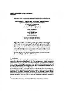
A pipeline is composed by a number n of stages, each stage i is separated with stages i − 1 and i + 1 by a register barrier. In a stage i , the input register barrier Ri , driven by xi is read and the treatment is executed; then the resulting information is recorded into the next register barrier Ri+1 , driven by xi+1 . We represent the pipeline flow control like a complete and deterministic Moore machine Mo = hSo , S0o , Io , Oo , To , Lo i. Each state represents a configuration of the pipeline stages where the computation is valid (and then written in the barrier register at the beginning of the next stage) or not. Transitions represent how the pipeline fills. Figure 1 represents a typical

pipeline flow. The control part contains a Moore Machine that (R2) If x0 = 1 or s is the initial state then ∃t ∈ To and produces the multiplexer command (xi ) driving the barrier ∃c ∈ C(Io ) such that t = (s, c, s0 ) and s0 = progress(0, s) register (Ri ) at the input of each stage. Two sets of registers and ∃t0 ∈ To ∃c0 ∈ C(Io ) such that t0 = (s, c0 , s00 ) and compose the barrier : one containing command (Ci ) and the s00 = progress(1, s). other data (Rdatai ) needed for the treatment into a stage. IV. I NCREMENTS APPLIED TO A PIPELINE FLOW The event handler generates events stalling or breaking the pipeline flow from internal or external signals. Data treatment The possible increments for a pipeline flow can be of two at each stage is represented by compi and transitions by ti . At types. The first type is an event, named stall, that introduces each step the register of a stage may take a new data coming deceleration in the pipeline flow. This is the case when the from the previous state, re-write its content or take an empty pipeline waits for a condition like a cache miss or a ready operation. An empty operation does not require any resource acknowledgment. The second type, named kill, concerns and do not disturb the state of the system. the pipeline flow breaks or reset. stage i-1

stage i

Ri Rdatai

stage i+1

Ri+1 Rdatai+1

compi

Ri+2

A. Single Stall

Rdatai+2 compi+1

Internal event Ci

∅

Ci+1

∅

ti

xi

∅

Ci+2

ti+1

xi+1

xi+2

Control part External event Event handler

Fig. 1.

Pipeline flow design

An event can stall a stage and all the stages upstream, the stages downstream progress and the stalled stages restart as soon as the stalling condition is not active anymore. The stalling condition is modeled by an event stallk = hstallk , stallk act, stallk qti. When stallk occurs then the (k + 1)th stage executes an empty operation; in all stages l > k, the flow progresses; in stages l ≤ k, the flow does not progress : each register Rl rewrites the value it previously stored. When stallk becomes inactive then the normal progression takes place (as defined by Rule R2). These new behaviours are modeled in a new Moore Machine Ms obtained by applying the incremental design process to Mo . Below we define the increment transforming Mo to Ms . We firstly introduce functions representing the prefix or suffix of a state. Definition 7: Prefix and Suffix functions. The function pref : IN× S → V0k associates to each state s and stage number k ∈ IN, the prefix of the state ranking from 0 to k. n The function suff : IN × S → Vk+1 associates to each state s and stage number k ∈ IN, the suffix of the state ranking from k + 1 to n − 1. Definition 8: Transition rules associated to stallk in Ms : Let s be a state in So . (R3) For all states s0 in So ,s.t. ∃t = (s, c, s0 ) ∈ To , then ∃t0 ∈ Td s.t. t0 = (s, c ∧ stallk qt, s0 ) (R4) ∃s00 6∈ So , s.t. ∃t = (s, stallk act, s00 ) and  R if xj = 1 (a) ∀x00j ∈ pref (k, s00 ): x00j = 0 if xj = 0 (b) suf f (k, s00 ) = progress(0, suf f (k, s))

The basic case we describe now is the optimal pipeline flow. The environment behaves ideally (no cache miss, no delaying actions). We define the set of vectors Vlk = xl , xl+1 , ..., xk−1 such that ∀j, xj ∈{0,1,R}. This represents a contiguous subset of the pipeline stages ranking from stage l to stage k. The states of a pipeline of n stages are in V0n . We have (x0 . . . xn−1 ) such that ∀j, xj ∈{0,1,R}. The meaning of these symbols is: • xj = 0 insertion of an empty operation in Rj . • xj = 1 insertion of the result of the computation of stage j − 1 in Rj . • xj = R re-writing of the Rj ’s content in Rj . Remark 2: In the basic case we consider that no event stalling a stage or freezing the pipeline may occur. In this case, the pipeline flow is regular and by consequence all states are labeled with an unique succession of consecutive 1. Definition 6: Progress function. The function progressk,l : {0, 1}×Vkl → Vkl is the right shift of any element in Vkl of 1 slot with either 0 or 1 injected in xk . Let be s ∈ Ss \ So . When there is no ambiguity the indexes k and l of progress (R5) ∃s0 s.t. (s, stallk qt, s0 ) and s0 is obtained by Rule R2. will be removed. Let t be in To , t is the conjunction of elementary transitions (R6) ∃s00 s.t. (s, stallk act, s00 ) and ti , each occurring at a given stage i of the pipeline, and (a) pref (k, s00 ) = pref (k, s), potentially driving register Ri . t ∈ To if and only if: (b) suf f (k, s00 ) = progress(0, suf f (k, s)) 00 0 0 Let be s = (xj )j∈[0;n−1] , s = (xj )j∈[0;n−1] and s = We state properties for the suffix and prefix functions. (x00j )j∈[0;n−1] then we have the following rules : Notation : x → x0 means ∃c ∈ C(I) and (x, c, x0 ) ∈ T . (R1) If x0 = 0 and if s is not the initial state then ∃t ∈ To and σ = y . . . y 0 is the path from y to y 0 such that y → y0 , y0 → ∃c ∈ C(Io ) such that t = (s, c, s0 ) and s0 = progress(0, s) y1 , . . ., yk → y 0 .

Property 1: Suffix progression. Let be a stall occurring at stage l or lower, inducing the machine Ms from Mo . Let Rl an binary relation in So × Ss such that: x Rl y iff suf f (l, x) = suf f (l, y). ∀x0 ∈ So s.t. x → x0 , ∃y 0 ∈ Ss s.t. y → y 0 and x0 Rl+1 y 0 . Proof: By construction of Ms Unfortunately, Rl+1 is not included into Rl , thus it is not a strong bisimulation [3]. Hence this property is local to the stall and expresses the progression of the suffix downstream, whenever the flow is broken upstream or not. Property 2: Prefix weak bisimulation. Let be a stall occurring at stage l or higher, inducing the machine Ms from Mo . Let Rl be a binary relation in So × Ss such that: xRl y iff pref (l, x) = pref (l, y). Rl is a weak bisimulation [3]. Proof: We have: ∀x0 ∈ So s.t. x → x0 , ∃y 0 ∈ Ss s.t. σ = y . . . y 0 and x0 Rl+1 y 0 . As pref (l + 1, x) = pref (l + 1, y) ⇒ pref (l, x) = pref (l, y), Rl+1 is included into Rl . ∀y 0 ∈ Ss s.t. y → y 0 s.t : x → x0 and x0 = y 0 (when y is not stalled and reads stalll qt), or (when y reads stalll act) x Rl y 0 and y 0 . . . y 00 and x0 Rl+1 y 00 . Rl+1 is included into Rl . Property 3: Stuttering progression. In Mo : We have σ = s0 s1 ...sn such that in sn : Vln+k = progressn (V0k ). In Ms : Let stallk be a stalling action occurring at stage k. Then ∃σ 0 = s∗0 s1 ...sn such that sn : Vln+k = progressn (V0k ). Proof: This is a direct consequence of rule R5 (assuming that the stalling action always terminates). B. Composition of Stall Increments In section IV-A we described the behaviours of the stepped up machine when taking into account the delays induced by a unique stall. However, it is possible to have events inducing stalls occurring at different stages. We define new transitions rules to model the dealing with multiple stalls. The transition rules are quite similar to the single stall increment we have seen before. But now, the order in which increments are added is important. The increment that affects the highest stages has a greater impact on the pipeline flow, than the increment concerning lower stages. Definition 9: Set of Stalls. Let be F = {k | k ∈ [0, n − 1]} the set of stages where a stall currently occurs. Let Ms0 be the machine obtained by applying on the machine Ms that contains already some stalls (defined in Fs ), a new stall at stage k s.t k > max(Fs ). Fs is augmented with k: Fs0 = Fs ∪ {k}. Ms0 is composed of states in Ss0 ⊃ Ss Definition 10: Transitions rules associated to Ms0 . Transitions in Ts0 ⊃ Ts are defined s.t.: •

• •

Let s be a state in Ss ∩ Ss0 . Its previously existing transitions are modified according to rule R3 with value stallk qt. Ms0 has got one new transition respecting rule R4 with value stallk act. Let be s ∈ Ss0 \ Ss ,

1) either s is the source state of the transition obtained by rule R6. 2) or (R5’) ∃s0 ∈ Ss0 s.t. (s, c ∧ stallk qt, s0 ) with c equal the conjunction of all stalll qt ∀l ∈ F \ {k} and s0 is obtained by Rule R2 (either a 0 or a 1 is injected at stage 0). 3) or (R7) ∀l ∈ F \ {k}, ∃s00 ∈ Ss0 s.t. (s, c ∧ 00 stallV k qt, s ) with c = ∀j∈[k;l[ stallj qt ∧ stalll act and with s00 : a) pref (l, s00 ) = pref (l, s) b) suf f (l, s00) = progress(0, suf f (l, s)). Remark 3: When we introduce a new increment stallk occurring at a stage k < max(Fs ) the active configuration is now ∀l ∈ Fs and l > k, stalll qt ∧ stallk act. This is because if a higher stall stalll is active, no matter stallk is also active, stalll freezes pref (l, s), that encompasses pref (k, s). Property 4: Let be a machine Ms0 obtained by multiple stall increments from Mo , having a set of stalls Fs0 . Let be l ≤ min(Fs0 ). Let Rl be the relation in So × Ss : x Rl y iff pref (l, x) = pref (l, y). 1) Rl is a weak bisimulation. 2) ∀ j > l, Rj is not a weak bisimulation. Proof: (sketch) The proof of the first statement proceeds as for the single stall increment case (property 2). The idea of the proof of the second statement is the following: In case of a single increment at stage l, the stages ranking from 0 to l − 1 have the same progression: either they are fixed (while stalll act), or they progress at the same speed (when stalll is not active anymore). This is captured by the weak bisimulation of the prefix Rl and the stuttering progression property. If l > min(Fs ), then there exists a stall , say k < l splitting the interval [0; l[ of stages into [0; k], where the behaviour is frozen until stallk is removed, while the stages ranking from k to l − 1 may progress. Hence the similarity of behaviours of stages in [0, l] are not captured in Rl anymore but in Rk (that is included in Rl ), and the stuttering progression property. C. Kill Increment A kill action destroys the treatment performed at a given stage, but the pipeline flow is not disrupted. The kill action is the basic operation performed in case of retract, reset, exception or interrupt. We will show in section VI how kills are used to manage these events. In our representation, a kill action consists in replacing the ”1” corresponding to the progression of the treatment by an empty operation ”0”. Definition 11: Let Ms be a machine, a kill event occurring at stage k induces the following machine Mk : Sk ⊃ Ss and Tk is defined such that: 1) ∀t ∈ Tk , t = (s, c, s0 ), t is changed into (s, c0 , s0 ) with c0 = c∧ killk qt. 2) ∀s ∈ Ss ∩ Sk , ∃s0 ∈ Sk and (s,killk act,s0 ) ∈ Tk and s’ is defined s. t. : x00 = 0 or 1, xk = 0 and ∀i 6= k, x0i = xi−1 .

V. C ONSEQUENCES ON CTL FORMULAE This section gives results on CTL property preservation or transformation between a reference machine and the one obtained by a composition of stall increments or a kill. In a first part, we consider properties with atomic propositions inside the pipeline. In a second part, we focus on properties concerning the macroscopic treatment performed by the pipeline. A. Properties related to the inner parts of the pipeline Let Ms be a machine obtained by composition of stall increments applied to Mo , and Fs be the set of associated stalls. Let Ms0 be the machine obtained by composition of stall increments applied to Ms and Fs0 (⊃ Fs ) be the set of associated stalls. We name φk (resp. φl ) an atomic proposition (or there negation) related to a stage k (resp. l) in Ms . From [5], the general transformations capturing the preservation of the behaviours of Ms in Ms0 due to any increment hold. From the previous paragraphs, the following properties hold: Property 5: Let f and g be any formula built from the following rules: • p = φk | φk ∨ φl | T RU E | F ALSE • fp = A p U fp | A fp U p | E p U fp | E fp U p | AGp | EGp | AGfp | EGfp • f = A f p U f | A f U f p | E fp U f | E f U f p | A f U g | E f U g | AGf | EGf | f ∨ g | f ∧ g Let Ms ,s |= f , we have Ms0 ,s |= f . Proof: (Sketch) This is due to the weak prefix bisimulation and the stuttering progression: let φk (resp. φl ) be a formula with atomic propositions related to stage k (resp. l), for any CTL\X operator OP, the formula of the form OP(φk )(resp. OPφl ) are preserved. Their disjunction is then preserved, and positive formulas built on their disjunction are also preserved. This is not true for the conjunction of atomic proposition concerning different stages (second item of property 4). Property 6: Let f and g be any formula built from the rules: • p = φk | φk ∧ φl | T RU E | F ALSE • f = Ap U f | Af U p | Af U g | Ep U f | Ef U p | Ef U g | f ∨ g | f ∧ g We have the following properties for k < l and a CTL\X operator OP: 1) if 6 ∃ i ∈ Fs0 s.t. i ≥ l, then Ms ,s |= f ⇒ Ms0 ,s |= f . 2) if ∃ i ∈ Fs0 s.t. i < l], and if ϕ = OP (φk ∧ φl ) then Ms ,s |= ϕ ⇒ Ms0 ,s |= ϕ0 and ϕ0 = OP (AF (φl ) ∧ φk ) Proof: Direct consequence of properties 3and 4. B. Properties related to the outer parts of the pipeline The environment of the pipeline is viewed as a set of actions composed of commands producing results. In case of a VCI-PI protocol converter ( [5]), it is composed of the set of VCI commands and of VCI responses. In case of a processor, the pipeline environment is composed of instructions on the software visible registers plus the program counter, instruction and exception registers, and the memory.

The environment is abstracted by a set E = {(Cmdk , Resk )}, where couples (Cmdk ,Resk ) denotes the k th command and its induced result. The causality between commands and results, and the interleaving of several actions are modeled by a set of CTL\X properties. A command Cmdk entering the pipeline may be expressed as: φ0,k = (x0 = 1 ∧ Ci = Cmdk ). Ci denotes the contents of a register in stage i. The end of the computation induced by Cmdk is expressed by: φn−1,k = (xn−1 = 1∧Cn−1 = Cmdk ) Example 1: A causality relation between Cmdk and Resk , expressed on the environment as Cmdk ⇒ AF Resk is transposed as: φ0 ⇒ AF (φn−1 ∧ AF Resk ). Property 7: All positive CTL\X formulas with atomic propositions in E, that are true in Mo , are also verified in any machine obtained by composition of stall increments. Proof: This is a direct consequence of property 5 that preserves positive CTL\X formulae when atomic propositions concern disjunction of stages (here concerned stages are 0 and n − 1). In case of a kill increment in a stage i, the command does not produce a result. In case of occurrence of a similar command not concerned with the kill event, a result similar to the one destroyed by the kill will be produced. A causality property expressed as Φk = φ0,k ⇒ AF (φn−1,k ∧ AF Resk ) can be transformed in the following form : Φ0k =¬killi ∧ φ0,k ⇒ A(¬killi U (Resk ∨ ^ (¬φl,k ) ⇒ AF ¬Resk ) ∨ (killi

(1) (2)

l∈[0;n−1]

(killi

_

(φl,k ) ⇒ AF Resk ))

(3)

l∈[0;n−1]

Line (1) expresses that there is some path where killi is never true due to the incremental design rules. Line (2) says that if a kill event occurred and no stage contains the command then the associated result is not produced. Line (3) corresponds to the occurrence of a similar command that produces a similar result. VI. I NCREMENTAL DESIGN

OF THE

VCI-PI

WRAPPER

In [5] we show how CTL property could be automatically transformed from a simple component in order to derive a part of the specification of a more complex one. Now, we want to take advantage of the increment particularity induced by the pipeline structure of the wrapper VCI-PI. In this part, we briefly recall the wrapper structure and then show how the formulae are transformed or preserved from properties of section V. The conversion between PI-bus and VCI protocols is realized by a component named a VCI-PI wrapper. A wrapper is a core wrapping device implementing a given interface. In our context, the IP-core is supposed to be VCI compliant [8] and the considered wrapper is an adapter between the VCI interface and the PI-bus protocol [13]; hence we are able to

VCI interface

PI bus interface

cmd cmd cmd cmd cmd cmd

pi req pi gnt

Master Wrapper pi pi pi pi pi

Fig. 2.

ad opc lock data ack

rsp rsp rsp rsp

VCI-PI

val eop ad ack data

val eop ack data

VCI and PI interfaces of our set of master wrappers (2)

Bus Arbitrer

(3)

VCI

(1) (10)

INITIATOR

VCI-PI master wrapper

(4)

P I

(9)

(3)

(5) (8)

B U S

VCI-PI slave wrapper

(6)

VCI

(7) TARGET

Fig. 3. The Platform performing the VCI-PI-VCI translation and illustration of a VCI transfer

connect various IP-cores through a PI-bus. PI protocol distinguishes the component initiating a bus transfer, named master, and the component responding to a transfer, named slave. An IP-core may have both master and slave functionalities. Figure 2 illustrates the major signals handled by interfaces of a VCIPI master wrapper. A VCI transfer is shown in Figure 3. The VCI initiator sends a request to the VCI-PI-master-wrapper (1), that asks for the bus to the bus arbiter (2), and when the VCI-PI-master-wrapper owns the bus (3), it transfers each VCI request cell through the PI-bus to the VCI-PI-slave-wrapper (4,5). The VCI-PIslave-wrapper translates the PI-cell into a VCI-cell to be given to the VCI target (6). The VCI-target transmits the VCIresponse to the VCI-PI-slave-wrapper (7), which responds to the VCI-PI-master-wrapper through the PI bus (8,9). This latter translates the PI-response into a VCI-response and sends it to the VCI initiator (10). In some cases, the VCI-PI-slavewrapper may implement a look-ahead mechanism in order to send the responses to the VCI-PI-master-wrapper in one cycle. Using the incremental design process approach, we developed a set of nine master VCI-PI wrappers, from a very simple one supposing that the VCI initiator and the PI target will always acknowledge in one cycle, up to the most complex one supporting delays, retract and reset events sent by the VCI initiator or the PI target. The hierarchy of the nine master wrappers is shown in Figure 4. The behavior of the simplest wrapper (model A) is a 3stages pipeline, performing at the same time: • accepting a VCI request k to be sent to PI from its VCI interface, th • sending the PI request corresponding to the k − 1 VCI request on its PI interface, th • accepting the PI response to the k − 2 VCI request on its PI interface. Further models (B to C”) deal with external events dis-

turbing the pipeline flow: either the k th VCI request can not be given to the wrapper, or the k − 1th response is delayed by the PI targets, or it says that a major problem occurred and the transaction has to be restarted later, or the k − 2th response can not be returned to the VCI initiator; all these cases stall or break the pipeline flow. For instance, we build a model B from the model A that take into account delay impose by the target. The new behaviour added corresponds to a stall action. We obtained the model B by applying definition 8. The new event corresponding to this extension is e = h(incb , {0, 1}), {0}, {1}i where CQT = {0} when pi rsp = RDY and CACT = {1} when pi rsp = W AIT . Model B’ is obtained by applying two increments from model A in respect to definition 10 with the increment e defined above and the increment e0 = h(incb0 , {0, 1}), {0}, {1}i. The event e0 represents the delay imposed by the master. The set of quiet configurations of e0 is CQT (incb0 ) = {0}. This configuration occurs when (cmd val = 1) ∧ (rsp ack = 1). The set of active configurations is CACT (incb0 ) = {1}, that occurs when (cmd val = 0) ∨ (rsp ack = 0). We implemented a platform as described in Figure 3 in synchronous Verilog. We checked about 80 CTL formulae for the master wrapper B, the slave wrapper B and the complete system (when the VCI initiator and target may generate delay events) with VIS verification tool [9] . Here are examples of CTL (untransformed) properties checked on the B platform. Formula 1 checks the interface between the VCI initiator and the wrapper: if 3 read cells are sent then the wrapper returns the response of the first cells and the acknowledgment of the third cells in the same cycle. Formula 2 checks the behavior of the complete system: the number of acknowledgment cells received by the VCI initiator is equal to the number of request cells it previously sent. Here, the initiator sends 2 requests. # formula 1: # AG( (cmd = READ_3_WORDS) -> AF( cmd_ack = 1 * rsp_val =1); # formula 2: # AG( (cmd = READ_2_WORDS) -> A ( (A ( (A((cmd = READ_2_WORDS * cmd_eop = 0 * cmd_val = 1) U (cmd_ack = 1))) U ( A( (cmd_eop = 1 * cmd_val= 1) U (cmd_ack = 1))))) U (cmd_val = 0) )); We fit the platform in order to plug a wrapper B’ obtained as described above. We reinforce our results by re-checking the set of all formulae written for the wrapper B. Of course, we transformed the formulae following the properties stated in section V. In practice, it is not useful to re-check formulae, we can obtain the new set of formulae by applying the increment rules and the properties transformation or preservation. Formula 1 contains a conjunction where atomics propositions concern stages 1 and 3. From B to B’ the increment may stall the stages 1 and 3, we apply Property 6. Formula 2 is

Type of event considered

Initiator is alway ready

Initiator may impose wait states

Initiator may ireset

cmd val=1; rsp ack=1

cmd val={0,1}; rsp ack = {0,1}

reset = {0,1}

Target is always ready pi rsp=RDY

A

A’

A”

Target may impose wait states pi rsp={RDY,WAIT}

B

B’

B”

C

C’

C”

Target may impose retract pi rsp={RDY,WAIT,RTR}

Fig. 4. Hierarchy of VCI-PI wrappers ranking from A to C”. Each arrow corresponds to an increment whose associated event is an extension of the definition domain of one or more signals.

a global property related to the outer part of the pipeline, by Property 7 it is preserved. The increment from B (resp. B’) to C (resp C’) corresponds to a new behaviour that breaks the pipeline flow. It’s a Kill increment that kills stages 1 and 2. The Reset increment is also a kill increment but it kills all requests that were in the pipeline. In this case the formulae have to be transformed with the property stated in [5]. New formulae can be automatically added to insure the preservation of non-reseted models into reseted one. These formulae state that after a reset occurrence, the converter returns into idle state and the pipeline is empty. VII. C ONCLUSION On the one hand, we have formalized an incremental method that is very close to those used by the designers. Our approach decomposes the complexity of building a pipeline flow from scratch by adding the different increments one by one. The designer has got a framework to focus on one difficulty at a time. Moreover this technique is not regressive, all behaviours of the component are preserved when a new increment is added. On the other hand we have shown that this method automatically derives the specification of a component from the specification of a simpler component. This specification is integrable into a general symbolic model checking process. By exploiting the behavioural characteristics that distinguish pipelines from other circuits we have particularized the pipeline increments and state new CTL formulae transformations. These transformations capture the behaviour that already existed and characterize the added behaviours. The approach we propose can be viewed of two different ways. Either the component is built applying the increments, it is guaranteed to respect the new specification, and it can be plugged as it is in a more complex system, its specification being used for compositional verification (assume-guarantee). Or the design is manually augmented (step by step) and the new specification is the one that the system has to comply with. This approach abstracts the control flow of a pipeline submitted to stall and kill actions. It will be interesting to use this abstraction instead of a real model in the development

of complex synchronized pipeline flows such as superscalar architecture or complex protocol converter where several pipelines have to cooperate. R EFERENCES [1] M. Aagaard. A Hazards-Based Correctness Statement for Pipelined Circuits. In CHARME’03, pages 66–80. Springer-Verlag LNCS 2860, 2003. [2] R. Alur, T. A. Henzinger, F.Y.C. Mang, S. Qadeer, S.K. Rajamani, and S. Tasiran. MOCHA: Modularity in Model Checking. In CAV’98: Proceedings of the 10th International Conference on Computer Aided Verification, volume 1427 of Lecture Notes in Computer Science, pages 521–525, London, UK, 1998. Springer-Verlag. [3] A. Arnold. Finite Transition Systems: Semantics of Communicating Systems. Prentice Hall International Ltd., Hertfordshire,UK, 1994. Translator-John Plaice. [4] M. Bozga, J-C. Fernandez, A. Kerbrat, and L. Mounier. Protocol ´ Verification with the ALDEBARAN Toolset. STTT, 1(1-2):166–184, 1997. [5] C. Braunstein and E. Encrenaz. CTL-Property Transformations along an Incremental Design Process. In AVOCS’04 - Proceedings of the 4th International Workshop on Automated Verification of Critical Systems, volume 128 of Electronic Note in Computer Science, pages 263–278. Elsevier, 2004. [6] J.R. Burch, E.M. Clarke, K.L. McMillan, D.L. Dill, and L.J. Hwang. Symbolic Model Checking: 1020 States and Beyond. Information and Computation, 98(2):142–170, 1992. Special issue for best papers from LICS’90. [7] J.R. Burch and D.L. Dill. Automatic Verification of Pipelined Microprocessors Control. In D.L. Dill, editor, Proceedings of the sixth International Conference on Computer-Aided Verification CAV’94, volume LNCS 818, pages 68–80, Standford, California, USA, 1994. SpringerVerlag. [8] On-Chip Bus Development Working Group. Virtual Component Interface Standard (VCI). VSI Alliance, 2000. [9] The VIS group. VIS : A System for Verification and Synthesis. In International Conference on Computer-Aided Verification, volume 1102 of Lecture Notes in Computer Science, pages 428–432. Springer-Verlag, 1996. [10] T.A. Henzinger, S. Qadeer, and S.K. Rajamani. You Assume, We Guarantee: Methodology and Case Studies. In Computer Aided Verification, volume 1427 of Lecture Notes in Computer Science, pages 440–451, London, UK, 1998. Springer-Verlag. [11] R. Hosabettu, M. Srivas, and G. Gopalakrishnan. Decomposing the Proof of Correctness of Pipelined Microprocessors. In Alan J. Hu and Moshe Y. Vardi, editors, Computer-Aided Verification, CAV’98, volume 1427, pages 122–134, Vancouver, Canada, 1998. Springer-Verlag. [12] J.K. Huggins and D. Van Campenhout. Specification and Verification of Pipelining in the ARM2 RISC Microprocessor. ACM Transactions on Design Automation of Electronic Systems, 3(4):563–580, 1998. [13] Open Microprocessors System Initiatives. OMI324: PI-Bus Standard Specification. Siemens, Munich, Germany, 1994.

[14] D. Kroening and W.J. Paul. Automated Pipeline Design. In DAC ’01: Proceedings of the 38th conference on Design Automation, pages 810– 815. ACM Press, 2001. [15] P. Manolios and S.K. Srinivasan. Automatic Verification of Safety and Liveness for XScale-Like Processor Models Using WEB refinements. In DATE ’04: Proceedings of the conference on Design, Automation and Test in Europe, pages 168–174, Washington, DC, USA, 2004. IEEE Computer Society. [16] H. Peng, S. Tahar, and F. Khendek. Comparison of SPIN and VIS for Protocol Verification. STTT, 4(2):234–245, 2003. [17] J. Sawada and W.A. Hunt. Trace Table Based Approach for Pipeline Microprocessor Verification. In CAV’97: Proceedings of the 9th International Conference on Computer Aided Verification, pages 364–375, London, UK, 1997. Springer-Verlag LNCS 1254.