Using Decision Trees and Text Mining Techniques for ... - CiteSeerX

Using Decision Trees and Text Mining Techniques for Extending Taxonomies Hans Friedrich Witschel [email protected] University of Leipzig, IfI, NLP Department, Augustusplatz 10/11, 04109 Leipzig, Germany

Abstract Lexical taxonomies have tree-like structures and can thus be extended to become decision trees that serve for their own extension. In this paper, a semi-automatic procedure for extending lexical taxonomies is proposed that makes use of term extraction methods for identifying new concepts and that uses cooccurrence data from large corpora to generate the necessary features (semantic descriptions) of the decision tree’s nodes.

1. Introduction Ontologies play an increasingly important role in many applications, especially in the Semantic Web. They are used for establishing common knowledge bases and making them readable to machines so that the knowledge can be applied automatically in many different contexts. However, the construction of ontologies can be a tedious, time-consuming and thus expensive process when performed manually. This article presents an idea of how certain text mining and machine learning techniques can be used to speed up the process of ontology engineering. An ontology can be defined as follows: ”An ontology is a formal specification of a shared conceptualisation” (Borst, 1997). This definition suggests that ontologies consist of concepts, i.e. classes of entities that are important for a given domain. Usually, these concepts can be structured hierarchically and thus form what linguists call a taxonomy. Taxonomies consist of concepts (or sets of words) arranged in a tree structure according to hyponymy (is-a) relations. Many linguistic ontologies like WordNet (Fellbaum, 1998) encode some additional semantic relations (like meronymy, antonymy etc.) and many Semantic Web ontologies have logical axioms or rules that allow to deduce further knowledge.

To summarize: ontologies (may) consist of: • A set of concepts • A hierarchy on these concepts • Additional (linguistic) relations between concepts and • Some logical axioms or rules In this paper, there will be a focus on extending taxonomies only because they are very important parts of every ontology. More precisely, the intention of this work is to outline an idea for combining statistical methods working on very large corpora with a machine learning approach (namely decision trees) to enrich a given taxonomy of concepts. In order to extend a given taxonomy, there are two tasks that have to be addressed: • Identifying new concepts and • Inserting these new concepts into the taxonomy at the right position The rest of this paper will be dedicated to examining related work and exploring new methods and algorithms that can be applied to solve these tasks. Finally, the process of inserting new concepts will be illustrated by an example followed by an evaluation of the proposed algorithm.

2. Related Work The task of extending existing lexical ontologies by analysing unstructured text has also been called ”ontology refinement” (cf. (Alfonseca & Manandhar, 2002b; Maedche & Staab, 2002)). Most of the approaches that have been followed in the domain can be roughly divided into two categories:

• Pattern-based methods that use regular expressions over unstructured text to identify hyponymy relations (cf. for instance (Hearst, 1998; Schnattinger & Hahn, 1998)): patterns may consist of very simple string matching (* is a * ) or use syntactical knowledge like selectional preferences of verbs. They can be produced manually or learned by analysing example sentences that include known pairs of hypernyms and hyponyms. The major drawbacks of these approaches result from poor precision, i.e. patterns will find too many pairs that are not related in the desired way. • Decision tree approaches have been proposed by (Alfonseca & Manandhar, 2002a) for extending WordNet with new concepts. They introduce socalled distributional (topic) signatures to describe concepts. These descriptions are then used to compute similarity between concepts. New concepts are inserted into an existing taxonomy tree by traversing it top-down, at each step descending via the most similar child of the current node, stopping when that node is more similar to the new concept than any of its children. 2.1. Contribution of this work The approach described in this paper is quite similar to the last of these methods. However, there are some important differences: rather than looking for plain similarities, i.e. simply categorising new concepts under the most similar synset encountered on the way down the tree, I will try to incorporate findings about the prevailing nature of relations found by certain cooccurrence statistics. This will lead to the use of more sophisticated statistics, but also to a different stopping criterion. I will also avoid methods that comprise linguistic knowledge (at least for the actual insertion of new concepts) because the use of shallow parsers and other language-specific techniques – as used by (Alfonseca & Manandhar, 2002a) – may prevent the algorithm from being applied to other languages. Finally, (Alfonseca & Manandhar, 2002c) recognize a serious problem: Top-level concepts normally have very general topic signatures that are not representative of their subconcepts. This leads to very homogenous similarity values when working with extensive signatures or even fails to produce matches when working with short ones. They tried to solve the problem by propagating semantic descriptions of nodes upwards to the next hypernym. My approach will be more radical in that the

upward-propagation of descriptions will be recursive, i.e. it will only stop when the root of the tree has been reached. Thus, matches are guaranteed and a node’s description is also representative of not only its children but also its grandchildren. Of course, this introduces other problems (which will be discussed later). Let us now turn to the ideas and algorithms that I propose for solving the task of ontology refinement.

3. Identifying concepts The selection of important concepts for a given domain is an indispensable prerequisite for ontology construction. This problem is very closely related to the task of term extraction so that we will use some term extraction techniques to tackle it (for simplicity, we will identify concepts with words at this stage). Following the ideas described in (Witschel, 2004), a combination of statistical and linguistic (i.e. patternbased) approaches is applied in order to find terminological single and multi-word units. The first step of the extraction process consists in the selection of a suitable text T (or a set of texts): it should be large, cover the main topics of the domain under inspection and use its specialised language. For the statistical approach, we need a so-called reference corpus R, which should be a very large, wellbalanced corpus covering most areas and terms of everyday language. Now, a statistical test is applied to every word w in T , measuring if its relative frequency in T is significantly above its relative frequency in R1 . The latter is considered as an approximation of the probability of occurrence of w in arbitrary texts. Or, put it another way: we try to extract words that appear (significantly) more often in a specialised language text than in everyday language. The observation that many terminological units (or concepts) are noun phrases of a characteristic form leads to a pattern-based extraction method: using a part-of-speech (POS) tagger, syntactic categories are assigned to each word. Now we can use regular expressions over POS tags to extract patterns like N N (noun noun) or A N (adjective noun). Multi-word units that match these patterns and appear with a certain frequency are often terminological noun phrases (cf. (Daille et al., 1994) and (Justeson & Katz, 1995)). Table 1 shows some single-word units and noun phrases extracted from the Microsoft Encarta entry on ”Air1 For the exact formulation of the statistical test, the reader is referred to (Witschel, 2004) and (Dunning, 1994)

Table 1. Single-word units and noun phrases extracted from Microsoft Encarta entry on ”Airplane”

Term airplane wing aircraft engine flight jet propeller fly fuselage supersonic Noun Phrase supersonic flight jumbo jet crop duster heavier-than-air craft space shuttle flight control

Frequency

Significance

152 84 46 47 45 35 15 27 14 13

1705 833 287 283 250 226 176 149 149 148

Frequency 7 5 3 4 5 3

plane”.

4. The decision tree approach 4.1. Background The calculation of associations from word cooccurrences in large corpora has become an interesting field of research (cf. (Heyer et al., 2001) or (Terra & Clarke, 2003)). In many approaches, a contextual description of a word w is derived by identifying other words that co-occur frequently with w in sentences or paragraphs. More precisely, to single out those words, statistical significance measures should be used which yield high values only for those words that co-occur with w more often than one would expect when assuming statistical independence and which are based on a proper mathematical model: (Dunning, 1994) proposes a likelihood ratio test which I will apply in my experiments. The distributional hypothesis (cf. (Harris, 1968)) states that whenever two words appear in many similar linguistic contexts, this implies semantic similarity. Therefore, in a second step, the set of words that cooccur frequently with w can be treated as a feature vector for w, representing its context. This context can be used for calculating word similarities which is normally done by somehow counting the number of common features within the vectors of two words (cf. (Terra & Clarke, 2003) or (Weeds et al., 2004)), e.g.

using the Dice coefficient. Now, the result of this second step will be another set of words to be associated with w, namely the ones the context vectors of which are highly similar to that of w. This set of words will later be called the semantic description of w. It contains words that are used in more or less the same contexts as w, i.e. there is a certain form of paradigmatic relation between them. Actually, it has been found that cohyponymy is the predominant relation type that is found by this procedure (cf. (Bordag, 2005) or (Bordag et al., 2005)), i.e. whenever two words are found to be similar in the way just described, there is a high probability that these words are cohyponyms (more precisely, the probability of the two words being cohyponyms is higher than for every other semantic relation). These findings will be highly useful when introducing a stopping criterion for my decision tree approach. Now that we have semantic descriptions for concepts, these can be compared – i.e. a similarity value for a pair of two concepts c1 and c2 can be computed – by simply counting the number of words that occur in the semantic description of both c1 and c2 . Since taxonomies are trees by nature, the idea of using them as decision trees was quite obvious. The problem was that for a taxonomy to become a decision tree, a set of suitable features is needed for each node. These features can, however, be derived from word similarities as described above: for each concept (or word) in the taxonomy, a description can be obtained by acquiring a set of semantically similar words (possibly cohyponyms). The next section describes how these descriptions can be used as features for a decision tree approach. 4.2. The Algorithm 4.2.1. Preparation: Before inserting any new concepts into a given taxonomy T , each node in T has to be enriched with its semantic description, i.e. a set of similar words, calculated as indicated above. Semantic descriptions are then propagated upwards, i.e. beginning with the leaves of the tree, each node transfers its description to its father node where it is merged with the father’s description. At the end of this propagation process, the root node contains all the words that have been associated with any one of the nodes beneath it.

4.2.2. Insertion:

4.4. Example

When inserting a new concept n (that has been identified as suggested in section 3), we first have to obtain its semantic description. We then perform the following actions in each step of the algorithm:

M¨obel (furniture) ALL

Schrank Tisch

1. The current node a is chosen (in the first step, a will be the root of the tree). We now inspect the set of all children C of a. 2. Let us assume that C consists of more than one element (if it does not, we insert the new concept n here, i.e. as a child of a). We now match the semantic description of n with the descriptions of each child node c ∈ C. There are two cases: • If the mean of the similarity values that we obtain is greater than their variance, this means that all children on this level are (roughly) equally similar to n so that we can deduce that the set C is the set of cohyponyms of n (we said above that semantic descriptions consist mostly of cohyponyms). This means that n has to be inserted here, i.e. as a child of a. • If the opposite is the case, then we go to step 1 and choose the most similar node c as the new a, i.e. we use c to further descend within the tree. This is done because we may assume that the cohyponyms of n are children (or grandchildren) of c: their descriptions have been propagated upwards during the preparatory phase and thus yielded the high similarity between the descriptions of c and n. The result of this procedure should be suggestions for insertion, i.e. a semi-automatic procedure involving human judgment should be applied that accounts for the uncertainty of the decisions described above. 4.3. Problems There is one main problem that might occur when applying this algorithm to a real taxonomy: When gathering related terms for a concept, we might include words that belong to different meanings of the original concept. This might provoke too many matches when descending down the tree: one does not know which direction to take. However, in this paper, there will be no suggestions for avoiding this problem, i.e. it will have to be left for future work. For now, we might assume that we are only dealing with taxonomies from specialised domains where ambiguity will not be a problem.

(table) Schreibtisch, Stuhl, Bett, Tresen, Sofa

Bett (bed) Hause, schlafen, Sofa, morgens, Schreibtisch

(cupboard) Wohnzimmer, Schreibtisch, Bett, Sofa, Regal, Tresor, Bargeld, Einbrecher, Geldkassette, Verkaufsraum, Tageseinnahmen Aktenschrank, T¨ ur

Garderobe (wardrobe) Schuhe, Schrank, Hosen, Kleid, Kost¨ um

Tresor (safe)

Aktenschrank

Bargeld, Einbrecher, Geldkassette, Verkaufsraum, Tageseinnahmen

(filing cabinet) T¨ ur

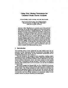
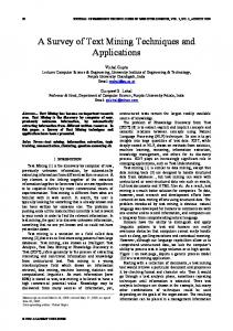
Figure 1. Parts of GermaNet subtree for ”M¨ obel” (furniture)

To illustrate how the algorithm works, I will present an example with a small subtree of GermaNet (the German equivalent to WordNet, cf. (Hampa & Feldweg, 1997)) and some co-occurrence data from the ”Deutsche Wortschatz” (Quasthoff, 1997). The data has been derived by using a likelihood ratio significance measure (Dunning, 1994) for evaluating co-occurrences and the Dice coefficient for calculating similarities between words using the feature vectors derived by the co-occurrence analysis. Fig. 1 depicts parts of the GermaNet subtree for ”M¨obel” (”furniture”). Each node is annotated with the five most significant items of its semantic description. The English translations of the concepts of this initial taxonomy are given in italics. In this example, we concentrate on inserting the new concept ”Safe” which is a German synonym of ”Tresor” (in GermaNet, however, it is classified as a hyponym to ”Tresor”). When looking up the semantic description of ”Safe”, we get: {Tresor, Bargeld, stahlen, Schmuck, entwendet, ...}. This means that, when looking at the children of ”M¨obel”, we get a similarity value of 2 for “Schrank” (because of the two matches with “Tresor” and “Bargeld” that have been propagated upwards) and values of 0 for all others. The mean (0.5) of those 4 values is smaller than their variance (which is 1), i.e. we descend via “Schrank”. In the second step, we compare with “Tresor” and “Aktenschrank”, obtaining similarity values of 2 and 0, respectively. Their mean (1) still being smaller than their variance (2), we further descend and attach the new concept as a hyponym of ”Tresor” (which is incidentally the position GermaNet assigns it).

5. Experiments and Results 5.1. Experimental Setup

for which no statistical data is available. It means that for each different value of t, the test set (i.e. the concepts to be inserted) had a different size.

5.1.1. Preparation In order to evaluate the proposed algorithm, experiments were conducted with the complete subtree from the example, i.e. the one for ”M¨ obel” in GermaNet. To facilitate the evaluation process, the multiple occurrence of concepts within the tree was ignored: synsets were only allowed to have one parent node within the hierarchy. If they did not, the first occurrence encountered when reading in the tree was chosen. When applying this restriction, the remaining subtree for ”M¨obel” consists of 145 synsets all of which were prepared in the manner described in section 4.2.1: for each word in the synset, related words were looked up in a previously calculated knowledge base and the synset was enriched with this information. In order to prepare the knowledge base, a huge amount of general-language texts (newspaper, fiction etc.) was analyzed, i.e. significance of word co-occurrences was calculated and each word was equipped with a ”context vector” containing the most significant co-occurrences of that word. These vectors were then compared using the Dice coefficient and similarity values for pairs of words were stored in a database. As mentioned above, these similarity values were then used to calculate descriptions for concepts (i.e. synsets). When computing these, a threshold t was applied: for each word in a synset, only the t most similar words were added to the description. We would expect the performance of the algorithm to improve when using more knowledge (i.e. when increasing t). But, of course, the statistical data is not perfect so that increasing t also introduces more noise which might actually degrade system performance. Therefore, t was varied in the experiments to study its effect on classification accuracy.

5.1.3. Evaluation metrics Two evaluation metrics were then used to assess the quality of the results: • The accuracy (or precision) of the decisions, i.e. the precentage of synsets that were correctly classified by the algorithm • The Learning Accuracy (LA): This measure is introduced by (Schnattinger & Hahn, 1998) and also used by (Alfonseca & Manandhar, 2002b) and measures not only the overall correctness of the final classification but also incorporates the distance between the position f predicted by the algorithm and the correct one s. This is done by looking for the lowest concept in the hierarchy that is a hypernym to both f and s2 . 5.2. Results Using the setup just described and varying the threshold t from 0 to 100, the values depicted in figure 2 were obtained. Note that, when using a threshold of t = 0, no knowledge is used so that each concept will be attached to the root node. We can consider that a baseline algorithm for our problem.

5.1.2. Classification In a second step, a subset of the 144 children and grandchildren of the root node ”M¨ obel” was selected. Each of the nodes in this subset was first removed from the tree – together with any subtrees attached to it, if present –and then re-inserted using the decision tree algorithm. The selection of synsets was based on the available knowledge: only those synsets, for which a description with a minimum size of t could be retrieved, were chosen. This was done because of the high uncertainty that is introduced when trying to classify new concepts

Figure 2. Results produced by the classification algorithm for the GermaNet subtree of ”M¨ obel” (furniture)

The label ”perc. of instances” refers to the number of concepts that were actually classified by the algorithm (i.e. that had sufficient statistical data associated with them). 2 For the exact definition of LA, the reader is referred to (Schnattinger & Hahn, 1998)

In a second run of experiments, I chose a bigger subtree of GermaNet, namely the one for “Bauwerk” (building), which consists of 902 nodes and is thus comparable in size to the tree that (Alfonseca & Manandhar, 2002a) used (they had 1200 nodes). Results for this subtree are shown in figure 3.

• When comparing accuracy for the two runs, we see a similar picture: the first run produces figures that are very close to the baseline whereas there are notable differences in the second run. The best accuracy values amount to 14% and 11% respectively, which is very poor (but comparable to the results of (Alfonseca & Manandhar, 2002a)). It suggests that we are still far from fully automatic classification: human intervention will surely be needed. • Finally, in both runs, the use of more than 20 features does not further improve the results (neither accuracy nor LA) which seems to indicate that a small amount of information is sufficient.

Figure 3. Results produced by the classification algorithm for the GermaNet subtree of ”Bauwerk” (building)

When comparing the results from the two different runs, we can make a number of interesting observations: • The statistical data – although computed from a huge amount of text (ca. 5 GB) – is sparse: for almost 60% of the instances from the “M¨ obel” subtree, it is not possible to retrieve a minimum of 10 (or more) similar words from the database. Although the situation is better for the “Bauwerk” subtree where the coverage does not drop that fast (with a coverage of 77% at t = 10), one might consider compiling a corpus consisting of a large amount of texts about “M¨ obel” or “Bauwerk” respectively and then computing statistics on that corpus. • Learning accuracy: In the “M¨ obel” example, there is no significant difference between the baseline (i.e. t = 0) and the best run of the algorithm. This means that classifying all nodes as hyponyms of the root node results in LA values that fall only slightly short of results obtained by more sophisticated methods. The situation is different for the bigger subtree where distances between nodes can be greater and the algorithm beats the baseline more obviously. Learning accuracy values are also higher in this scenario. All in all, the LA values obtained are quite significantly better than those reported in (Alfonseca & Manandhar, 2002a).

Unfortunately, it seems very difficult to compare results to those of other approaches: even if they use the same evaluation metrics, the quality of the classification results depends heavily on the concepts chosen for insertion and – as we have seen – also on the subtree one uses. The fact that (Alfonseca & Manandhar, 2002a) use completely new concepts (i.e. ones not previously contained in the taxonomy) makes it impossible for them to apply objective criteria: decisions have to be evaluated manually which is somewhat subjective. On the other hand, the taxonomies used (e.g. GermaNet) were also constructed manually so that some positions of synsets within the GermaNet tree might be arguable. To name just one example: in GermaNet, all “institutions” are possible hyponyms of “Bauwerk” (building), i.e. every institution can also be a building. Thus, words like “Gesundheitswesen” (“health care” – which is classified as a “national institution”) are also buildings. It is very questionnable whether a good classification algorithm should really reproduce this. As a consequence, it seems difficult to draw conclusions from the figures presented in this section. If any, one might deduce that the task of extending taxonomies is inherently difficult and that using large amounts of statistical data (e.g. more than 20 related words) for each concept does not significantly improve results. A closer qualitative examination of the problems involved in this task will be conducted in the next subsection. 5.2.1. Qualitative Analysis To get a better understanding of the nature of problems and in order to simplify the setting, a very simple experiment was conducted: an artificial taxonomy was formed by attaching two (quite, but not completely different) GermaNet subtrees to a new and artificial root

node. This taxonomy was then used in the same way as described above (with t = 20), but this time only the first step of the classification task was examined: did the algorithm choose the right subtree, i.e. could it categorize concepts correctly and thus differentiate between just two different concepts? To measure the algorithm’s performance in this setting, I used the measures precision and recall : since the algorithm did not always step down into one of the subtrees, recall indicates how many instances were actually classified, whereas precision denotes the percentage of correct decisions among those elements that were classified. The experiment was applied to two different settings: in a first run, the new tree was more or less balanced, i.e. the subtrees for “M¨ obel” (144 nodes) and “Kunstwerk” (work of art, 94 nodes) were combined. In a second run, the subtree for “M¨ obel” was paired with the much bigger one for “Bauwerk” (building – with 902 nodes) so that the resulting tree was fairly imbalanced. Note that all three subtrees are siblings in GermaNet which means that the differentiation between them should not be completely trivial. A simpe baseline for this task consists in classifying all nodes under the bigger subtree. This baseline performs – of course – quite good for the imbalanced tree and worse for the balanced one and always has a recall of 100%. The results of the simple classification task are shown in tables 2 and 3, with precision and recall values for both trees separately (precision for the “M¨obel” subtree, for instance, indicates how many of the M¨obel instances were correctly classified).

M¨obel Kunstwerk Overall Baseline

Precision 87.5% 94.7% 91.9% 55.4%

Recall 58.5% 74.5% 67.4% 100%

Table 2. Precision and recall for subtrees “M¨ obel” (furniture) and “Kunstwerk” (work of art)

We can see from the overall values that precision is high, which means that most of the decisions the algorithm took were correct. On the other hand, recall is quite low (between 67% and 79%) which indicates that, in many cases, the algorithm gives up too soon. Another interesting problem can be observed by comparing the precision values of the “M¨ obel” subtree in the two scenarios: when paired with another tree

M¨obel Bauwerk Overall Baseline

Precision 42.9% 100% 97.8% 92.8%

Recall 42.9% 82.1% 79.3% 100%

Table 3. Precision and recall for subtrees “M¨ obel” (furniture) and “Bauwerk” (building)

of roughly equal size, precision is quite high (88%) whereas it drops to only 42.9% when combined with a bigger subtree. This suggests that there is a bias towards the bigger subtrees, which results from calculating similarities between concepts as the pure number of common words in their descriptions: the upward propagation of concepts leads to very extensive descriptions for concepts that have large subtrees beneath them. This introduces noise and results in high (and possibly incorrect) similarity values when compared to arbitrary concepts. Unfortunately, the normalization of similarity values with a concept’s size did not improve results when I tried to apply it in a second run of experiments. The complexity of the problem results from the fact that a certain bias towards large subtrees (as a prior probability) is desirable, but must be balanced with the noise that it introduces.

6. Future work The results in the previous section have shown that much remains to be done in the future: the problem of ambiguous concepts should be considered and tackled. It would also be a good idea to provide a standard test bed for different extension algorithms that is free of human decisions (as far as that is possible). The method proposed in this paper – being a sort of n-fold cross-validation on the existing tree (where n is the number of nodes in it) – could be used and applied to the other approaches in the literature in order to obtain comparable results. Finally, the effect of choosing different corpora for the calculation of statistical co-occurrence data should be analyzed: one would expect that calculating cooccurrences from domain-specific texts (instead of general-language corpora) should solve the problem of data sparseness, at least when extending taxonomies for that domain.

7. Conclusion In this paper, a novel technique for extending lexical taxonomies was introduced that uses large corpora to identify concepts and calculate word similarities and a machine learning approach (decision trees) together with these similarities to insert new concepts at the right position of the tree. The mode of operation of this algorithm was shown by an example and evaluated using two different subtrees from GermaNet. Results show that (for reasonnably large trees) the classification and learning accuracy can be improved quite significantly when compared to a baseline algorithm that classifies all new concepts as direct hyponyms of the root node. However, the overall classification accuracy was still very poor in both test cases, which suggests (once again) that the automatic extension of lexical taxonomies is still a very difficult problem and that without human intervention, it will fail to reach acceptable performance.

References Alfonseca, E., & Manandhar, S. (2002a). Extending a lexical ontology by a combination of distributional semantics signatures. Proc. of EKAW-2002 (pp. 1– 7). Alfonseca, E., & Manandhar, S. (2002b). Proposal for evaluating ontology refinement methods. Proc. of LREC 02. Alfonseca, E., & Manandhar, S. (2002c). An unsupervised method for general named entity recognition and automated concept discovery. Proceedings of the 1st International Conference on General WordNet. Bordag, S. (2005). Algorithms extracting linguistic relations and their evaluation. Bordag, S., Witschel, H., & Wittig, T. (2005). Evaluation of lexical acquisition algorithms. Proc. of GLDV 2005 (pp. 449–461). Borst, W. (1997). Construction of engineering ontologies. Doctoral dissertation, University of Twente, Enschede. Daille, B., Gaussier, E., & Lange, J. (1994). Towards automatic extraction of monolingual and bilingual terminology. Proc. of COLING 94 (pp. 515–521). Dunning, T. (1994). Accurate methods for the statistics of surprise and coincidence. Computational Linguistics, 19, 61–74.

Fellbaum, C. (1998). Wordnet: an electronic lexical database. Cambridge, Mass.: MIT Press. Hampa, B., & Feldweg, H. (1997). Germanet – a lexical-semantic net for german. Proc. of ACL workshop Automatic Information Extraction and Building of Lexical Semantic Resources for NLP Applications, Madrid. Harris, Z. (1968). Mathematical structures of language. New York: Interscience Publishers John Wiley & Sons. Hearst, M. (1998). Automated discovery of wordnet relations. In Wordnet: an electronic lexical database. Cambridge, Mass.: MIT Press. Heyer, G., L¨auter, M., Quasthoff, U., Wittig, T., & Wolff, C. (2001). Learning relations using collocations. Proceedings of the IJCAI Workshop on Ontology Learning (pp. 19–24). Justeson, J., & Katz, S. (1995). Technical terminology: some linguistic properties and an algorithm for identification in text. Natural Language Engineering, 1, 9–27. Maedche, A., & Staab, S. (2002). Measuring similarity between ontologies. Proc. of EKAW 2002 (pp. 251– 263). Quasthoff, U. (1997). Projekt der deutsche wortschatz. Proc. of GLDV97 (pp. 93–99). Schnattinger, K., & Hahn, U. (1998). Towards text knowledge engineering. Proc. of AAAI ’98 / IAAI ’98 (pp. 524–531). Terra, E., & Clarke, C. L. A. (2003). Frequency estimates for statistical word similarity measures. HLTNAACL 2003 (pp. 165–172). Weeds, J., Weir, D., & McCarthy, D. (2004). Characterising measures of lexical distributional similarity. Proc. of COLING-2004. Witschel, H. (2004). Terminologie-extraktion – M¨ oglichkeiten der Kombination statistischer und musterbasierter Verfahren. W¨ urzburg: Ergon Verlag.