Incremental Tree-Based Missing Data Imputation with Lexicographic Ordering Claudio Conversano Department of Economics University of Cassino Via M. Mazzaroppi, I-03043 Cassino (FR), Italy
[email protected]
Roberta Siciliano Department of Mathematics and Statistics University Federico II of Naples Via Cinthia, Monte Sant’Angelo, I-80126, Napoli, Italy
[email protected] October 2, 2003
Abstract. In the framework of data imputation, this paper provides a non-parametric approach to missing data imputation based on Information Retrieval. In particular, an incremental procedure based on the iterative use of a tree-based method is proposed and a suitable Incremental Imputation Algorithm is introduced. The key idea is to define a lexicographic ordering of cases and variables so that conditional mean imputation via binary trees can be performed incrementally. A simulation study and real world applications are shown to describe the advantages and the good performance with respect to standard approaches1 Keywords: Missing Data, Tree-based Classifiers, Regression Trees, Lexicographic Order, Nonparametric Imputation, Data Editing.
1
The work has benn realized within the framework of the Research Project ”‘INSPECTOR”’, Quality in the Statistical Information Life-Cycle: A Distributed System for Data Validation, supported by the European Community, Proposal/Contract no.: IST-200026347.
1 1.1
Introduction Background
Missing or incomplete data are a serious problem in many fields of research because they can lead to bias and inefficiency in estimating the quantities of interest. The relevance of this problem is strictly proportional to the dimensionality of the collected data. Particularly, in data mining applications a substantial proportion of the data may be missing and predictions might be made for instances with missing inputs. In recent years, several approaches for missing data imputation have been presented in the literature. Main reference in the field is the Little and Rubin book (1987) on statistical analysis with missing data. An important feature characterizing an incomplete data set is the type of missing data patterns: if variables are logically related, patterns follow specific monotone structures. Another important aspect is the missing data mechanism which takes into account the process generating missing values. In most situations, a common way for dealing with missing data is to discard records with missing values and restrict the attention to the completely observed records. This approach relies on the restrictive assumption that missing data are Missing Completely At Random (MCAR), i.e., that the missing-ness mechanism does not depend on the value of observed or missing attributes. This assumption rarely holds and, when the emphasis is on prediction rather than on estimation, discarding the records with missing data is not an option (Sarle, 1998). An alternative and weaker version of the MCAR assumption is the Missing at Random (MAR) condition. Under a MAR process the fact that data are missing depends on observed data but not on missing data themselves. While the MCAR condition means that the distributions of observed and missing data are indistinguishable, the MAR condition states that the distributions differ but missing data points can be explained (and therefore predicted) by other observed variables. In principle, a way to meet the MAR condition is to include completely observed variables that are highly related to the missing ones. Actually, most of the existing methods for missing data imputation discussed in Shafer (1997) just assume the MAR condition and, in these settings, a common way to deal with missing data are conditional mean methods or model imputation, i.e., to fit a model on the complete cases for a given variable treating it as the outcome and then, for cases where this variable is missing, plug-in the available data in the model to get an imputed value. The most popular conditional mean method employs least squares regression (Little, 1992) but it can be often unsatisfactory for nonlinear data and biased if model misspecification occurs. Other examples of model-based imputations are logistic regression (Vach, 1994) or generalized linear models (Ibrahim, et al., 1999).
1.2
The key idea
In the framework of model-based imputation, parametric as well as semiparametric approaches can be unsatisfactory for nonlinear data and yield to biased estimates if model misspecification occurs. This paper provides a methodology to overcome the above shortcomings when dealing with the monotone missing data pattern assumption within the missing at random mechanism. The idea is to consider a non-parametric approach such as tree-based modelling. As well known, exploratory trees can be very useful to describe the dependence relationships of a response or output variable Y given a set of predictors or inputs. At the same time, decision trees can be fruitfully considered to classify or to predict the response of unseen cases. In this respect, we use decision trees for data imputation when dealing with missing data. The basic idea of the proposed methodology is as follows: given a variable for which data needs to be imputed, and a set of other observed variables, the method considers the former as response and the latter as predictors in a tree-based estimation procedure. Indeed, terminal nodes of the tree are internally homogeneous with respect to the response variable providing candidate imputation values for this variable. In order to deal with imputations in many variables we introduce an incremental approach based on a suitably defined pre-processing schema, generating a lexicographic ordering of different missing values. The key idea is to rank missing values that occur in different variables and deals with these incrementally, i.e, augmenting the data by the previously imputed values in records according to the defined order.
1.3
The structure of the paper
This paper is structured into two methodological sections and two other sections for the empirical evidence and discussion of the results, in addition to the present introduction and the final conclusions. In section 2, we present a suitable tree-based method to define decision rules for missing data imputation. Particular attention is payed to the FAST splitting algorithm for computational cost savings. In section 3, we introduce the incremental tree-based approach for conditional data imputation using lexicographic ordering. Both methodological and computational issues will be discussed and the Incremental Imputation Algorithm (IIA) will be introduced. Section 4 shows the results of a simulation study encouraging the use of the proposed methodology when dealing with nonstandard and complex data structures. Section 5 provides the results of practical applications of the proposed approach using well known data sets derived from the machine learning repository. The performance of the proposed methodology in
both simulations and real world applications will be compared to standard approaches to data imputation.
2 2.1
Tree-based methods Growing exploratory trees
Let (Y, X) be a multivariate random variable where X is the vector of M predictors of numerical or categorical type and Y is the response variable taking values either in the set of prior classes C = {1, . . . , j, . . . , J} (if categorical) - yielding to classification trees - or the real space (if numerical) yielding to regression trees. Basically, any tree-based methodology consists of a data-driven procedure called segmentation, that is a recursive partitioning of the feature space yielding to a final partition of cases into internally homogeneous groups, where a simple constant model is fitted in each group. In the following, we restrict our attention to binary partitions and thus binary trees which will be considered in the proposed incremental approach for data imputation. From an exploratory point of view, an oriented tree graph allows to describe conditional paths and interactions among those predictors to explain the response variable. Indeed, data are partitioned by choosing at each step a predictor and a cut point along it, generating the most homogeneous subgroups respect to the response variable according to a goodness of split measure. The heterogeneity of Y in any node t is evaluated by an impurity measure iY (t), i.e., the heterogeneity Gini index or the entropy measure for classification trees, the variation for regression trees. The best split at any node t can be found minimizing the so-called local impurity reduction factor: ωY |s (t) =
X
iY (tk , s)p(tk |t, s)
(1)
k
for any split s ∈ S provided by splitting the input features, and children nodes k = 1, 2, where p(tk |t, s) is the proportion of observations that pass from the node t to the sub-group tk due to the split s of the input features. It is also possible to define a boundary value to the local impurity reduction factor that cannot be improved by any split. The lowest value is reached by the optimal theoretical split of the cases looking at the splitting retrospectively, without considering the predictors. In other words, it is determined by the split of objects that minimizes the internal heterogeneity of Y into the two sub-groups discarding the input features. If there exists an observed split of the input features which provides the optimal split of the cases then the best split is also an optimal one (for further details see Siciliano and Mola, 2002). In the other cases, the ratio between the local impurity reduction factor provided by the best split over that one provided
by the optimal split can be interpreted as a relative efficiency measure of the split optimality. Applying recursively the splitting criterion allows to minimizing the total tree impurity: IY (T ) =
X
iY (h)p(h)
(2)
˜ h∈H
where H is the set of terminal nodes of the tree, each including a proportion p(h) of observations. Once the tree is built, a response value or a class label is assigned to each terminal node. In classification trees, the response variable takes value in a set of previously defined classes, so that the node is assigned to the class which presents the highest proportion of cases. In regression trees, the value assigned to the objects of a terminal node is the mean of the response variable values associated with the cases belonging to the given node. Note that, in both cases, this assignment is probabilistic, in the sense that a measure of error is associated with it.
2.2
FAST splitting algorithm
The goodness of split criterion based on (??) express in different way some equivalent criteria which are present in most of the tree-growing procedures implemented in specialized softwares; for instance, CART (Breiman, et al., 1984), ID3 and CN4.5 (Quinlan, 1993). In our methodology, the computational time consuming spent by a segmentation procedure is crucial so that a fast algorithm is required. For that, we recall the two-stage splitting criterion which considers the global role played by the predictor in the binary partition. The global impurity reduction factor of any predictor Xm is defined as: ωY |Xm (t) =
X
iY |g (t)p(g|t)
(3)
g∈Gm
where iY |g (t) is the impurity of the conditional distribution of Y given the m-th modality of Xm for Gm the number of modalities of Xm and m ∈ M . Two-stage finds the best predictor(s) minimizing (??) and then the best split among the splits of the best predictor(s) minimizing the (??) taking account of only the partitions or splits generated by the best predictor. This criterion can be applied either sic et simpliciter or considering alternative modelling strategies in the predictor selection (an overview of the two-stage methodology can be found in (Siciliano and Mola, 2000). The FAST splitting algorithm (Mola and Siciliano, 1997) can be applied when the following property holds for the impurity measure: ωY |Xm (t) ≤ ωY |s (t) for any s ∈ Sm of Xm . The FAST algorithm consists of two basic rules:
• iterate the two-stage partitioning criterion using (??) and (??) selecting one predictor at a time and each time considering the predictors that have not been selected previously; • stop the iterations when the current best predictor in the order X(v) at where iteration v does not satisfy the condition ωY |X(v) (t) ≤ ωY |s∗ (v−1) ∗ s(v−1) is the best partition at iteration (v − 1). The fast partitioning algorithm finds the optimal split but with substantial time savings in terms of the reduced number of partitions or splits to be tried out at each node of the tree. Simulation studies show that in binary trees the relative reduction in the average number of splits analyzed by the fast algorithm with respect to the standard approach increases as the number of predictor modalities and the number of observations at a given node increase. Further theoretical results about the computational efficiency of the fast-like algorithms can be found in Klaschka, et al. (1998).
2.3
Decision tree induction
The exploratory tree procedure results in a powerful graphical representation which express the sequential grouping process. Exploratory trees are accurate and effective with respect to the training data set used for growing the tree but they might perform poorly when applied for classifying/predicting fresh observations which have not been used in the growing phase. To satisfy an inductive task, a reliable and parsimonious tree (with a honest size and high accuracy) should be found to be used as decision-making model for nonstandard and complex data structures. A possible approach is to grow the totally expanded tree and remove retrospectively some of the branches considering a down-top algorithm called pruning. The training set is often used for pruning whereas cross-validation is considered to select the final decision rule (Breiman et al.). In order to define the pruning criterion it is necessary to introduce a measure C ∗ (.) that depends on both the size (number of terminal nodes) and the accuracy (error rate or Gini index for classification tree and mean square error for regression tree). Let Tt be the branch departing from the node t having |T¯t | terminal nodes. In CART the following cost-complexity measure is defined respectively for the node t and for the branch Tt as Cα (t) = Q(t) + α, Cα (Tt ) =
X h∈|T¯t |
Q(h) + α|T¯t |,
(4) (5)
where α is the penalty for complexity due to one extra terminal node in the tree, Q(·) is the node accuracy measure and |T¯t | is the number of terminal nodes of Tt . The idea of CART pruning is to prune recursively the branch Tt that provides the lowest reduction in accuracy per terminal node (i.e., the weakest link) as measured by αt =
Q(t) − Q(Tt ) |T¯t | − 1
(6)
that is evaluated for any internal node t. As a result, a finite sequence of nested pruned trees can be found T1 ⊃ T2 ⊃ . . . Tq ⊃ {t1 } and the final decision rule is selected as the one which minimizes the five- or tenfold cross-validation estimate of the accuracy (Hastie, et al., 2001). A statistical testing procedure can be also adopted in order to define a reliable honest tree, validating in this way the pruning selective selection made with CART (Cappelli, et al., 2002).
3 3.1
The incremental approach for data imputation The lexicographic ordering for data ranking
The proposed imputation methodology is based on the assumption that data are missing at random so that the mechanism resulting in its omission is independent of its unobserved value. Furthermore, missing values often occur for more variables. Let X be the n×p original data matrix, where there are d < p completely observed variables and m < n complete records. For any row of X, if q = p − d is the number of variables with missing data, which maximum P value is Q = (p − d + 1), there might be up to k (Q q ) types of missing-ness, ranging from the simplest case where data are missing for only one variable to the hardest condition to deal with, where data are missing for all the Q variables. Define the matrix R to be the indicator matrix with ij-th entry 1 if xij is missing and zero otherwise. Summing up over the rows of R yields to the p-dimensional row vector c which includes the total number of missing values for each variable. Summing up over the columns of R yields to the n-dimensional column vector r which includes the total number of missing values for each record.
A B C D E
F G H
I
J
K L M N O P Q R S T U V W X Y Z
1 2 3 4 5 6 7 8 9 10 11 12 13 14 15
0 3 0 0 0 2 1 3 0 1 3 2 0 0 2
A C E H I
M O P S V W Y B D G J
A C E H I
M O P S V W Y B D G J
K L Q R T U X Z N F
1 2 3 4 5 6 7 8 9 10 11 12 13 14 15
0 1 0 1 0 3 1 0 0 1 1 1 0 2 0 0 1 1 0 1 1 0 0 1 0 1
b)
a) A C E H I
M O P S
V
W Y
B D G J K L Q R T U X Z N F
0_mis 0_mis 0_mis 0_mis 0_mis 0_mis 0_mis 1_f 1_l 1_j 2_u_f 2_d_j 3_t_n_f 3_b_l_n 3_d_r_z
1 3 4 5 9 13 14 7 10 6 12 15 2 8 11
c)
K L Q R T U X Z N F
0_mis 0_mis 0_mis 0_mis 0_mis 0_mis 0_mis 0_mis 1_l 1_j 2_u_f 2_d_j 3_t_n_f 3_b_l_n 3_d_r_z
1 3 4 5 9 13 14 7 10 6 12 15 2 8 11
d)
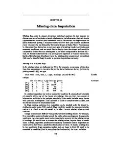
Figure 1. An illustration of the incremental imputation process: a) original data matrix; b) data rearrangement based on the number of missingness in each column; c) data rearrangement based on the number of missingness in each row and definition of the lexicographical order; d) the rearranged data matrix after the first iteration of the imputation process.
We perform a two-way re-arrangement of X, one with respect to the columns and one with respect to the rows. This re-arrangement allows to define a lexicographic ordering (Cover and Thomas, 1991; Keller and Ullman, 2001) of the data that matches the ordering by values, namely by the number of missing values occurring in each row and column of X. In particular, the re-arrangement satisfies the following missing data ranking conditions, respectively for the rows and for the columns: r1 ≤ r2 ≤ . . . ≤ rn
(7)
c1 ≤ c2 ≤ . . . ≤ cp
(8)
being ri the entry of r and
being cj the entry of c. In this way, the variables and the records are both sorted in terms of number of missing values as well as of column occurrence. By definition, it holds that ri = 0 for i = 1, . . . , m and cj = 0 for j = 1, . . . , d. The resulting re-arranged data matrix denoted by Z can be viewed as partitioned into four disjoint matrices:
Am,d
Cm,p−d
Zn,p =
Bn−m,d Dn−m,p−d where only the matrix D contains missing values while the other three blocks are completely observed in both rows and columns. By definition, within the uncomplete block D missing values are placed at different degrees of missing-ness from the right to left and from the upper part to the bottom part. In particular, if there exists only one variable presenting only one missing data, then this variable results in the p-th column and the first imputed value will be found for the m + 1-th record. If there are two variables with only one missing data then they are in the last two columns, and the first imputed values will be found in the m+1-th record. A graphical representation of the above data pre-processing yielding to the matrix Z is given in figure 1.
3.2
The incremental imputation method
Once that the different types of missing-ness have been ranked and coded, the missing data imputation is iteratively made using tree based models. The general idea is to use the complete part of Z to impute - via decision trees - the uncomplete one D, and on the basis of the lexicographic ordering the imputed values enter in the complete part for the imputation of the remaining missing values. In practice, the matrix Z can be viewed as structured into two submatrices Z = [Zobs |Zmis ], where Zobs is the n × d complete part and Zmis is the n × (p − d) uncomplete part. The latter is formed by the q = (p − d) variables presenting missing values, namely Zmis = [Zd+1 , . . . , Zp ]. With respect to the records presenting only one missing data, a simple tree is used. Applying the tree-based procedure, each variable presenting missing values is considered as response variable at turn, whereas the remaining variables presenting either no missing values or imputed values are used as predictors. Whereas the first d variables in Zobs always enter as predictors, the last q variables might enter either as a response or as a predictor in the tree procedure. The decision tree is obtained applying crossvalidation estimates of the error rate and considering the current complete sample of objects. The results of the tree are used to impute the missing data in D. In fact, terminal nodes of the tree represent candidate imputed values. Actual imputed values are get by dropping down the tree the cases of B corresponding to the missing values in D (for the variable under imputation), till a terminal node is reached. The conjunction of the filled-in cells of D with the corresponding observed rows in B generates new records which are appended to A, that gains the rows whose missing values have
been just imputed and a “new” column corresponding to the variable under imputation. For records presenting multiple missing values, trees are used iteratively. In this case, according to the previously defined lexicographic ordering, the tree is first used to fill in the missing values of the variables presenting the smallest number of incomplete records. The procedure is then repeated for the remaining variables under imputation. In this way, we form as many trees as the number of variables with missing values in the given missingness. In the end, the imputation of joint missing-ness derives from subsequent trees. A graphical description of the imputation of the first missing value is given in figure 2.
Figure 2. An illustration of the incremental imputation process: after the first iteration the row 10 becomes completely observed and the imputation process proceed through imputation of row 6.
A formal description of the proposed imputation process at any generic vth iteration can be given as follows. Let yi∗ ,j ∗ be the cell presenting a missing input in the i∗ -th row and the j ∗ -th column of the matrix Z. The imputation derives from the tree grown from the sample Lv = {x0i , yi ; i = 1, . . . , s} where yi = zij ∗ and x0i = (zi,1 , . . . , zi,j , . . . , zi,p )0 such that rij = 0 for any couple (i, j). The imputation of the current missing data zi∗ j ∗ is obtained from the decision rule d(x) = y. Obviously due to the lexicographical order the imputation is made separately for each set of rows presenting missing data in the same cells.
As a result, this imputation process is incremental, because as it goes on more and more information is added to the data matrix, both respect the rows and the columns. In other words, the matrices A, B and C are updated in each iteration, and the additional information is used for imputing the remaining missing inputs. Equivalently, the matrix D containing missing values shrinks after each set of records with missing inputs has been filledin. Furthermore, the imputation is also conditional because, in the joint imputation of multiple inputs, the subsequent imputations are conditioned on previously filled-in inputs.
3.3
The Incremental Imputation Algorithm (IIA)
From the computational point of view, some issues need to be considered in order to implement the proposed imputation procedure. Actually, the data re-arrangement of the matrix X yielding to Z is performed only at the beginning of the procedure, resulting in a data preprocessing step. In sub-sequent iterations, instead of sorting rows and columns of Z, the ri and the cj , in the conditions (??) and (??) respectively, are updated and used as pointers to identify the data under imputation. It results that the procedure stops when all the ri and the cj become zero. It is worth mentioning a specific property derived from the lexicographic ordering to rank missing data in each row of the matrix Z. At any v-th iteration, the procedure takes account of the row with the lowest number of missing data. It can be shown that if a missing data is imputed within the i∗ -th record then it follows that, in the subsequent iteration v + 1, any further missing data within the same record will be necessarily imputed. In the following, we outline the Incremental Imputation Algorithm (IIA) implementing the proposed methodology. 0. : Pre-Processing: Missing Data Ranking. Let X be the data matrix. Define the indicator matrix R with ij-the entry 1 if xij = 0 and zero otherwise. Define the column vector r = R1 being the ri entry the number of missing values in the i-th record. Define the row vector c = 1R being the cj entry the number of missing values in the j-th variable. Apply the missing data ranking conditions (??) and (??) to the matrix X for both rows and columns in order to define the matrix Z = [Zobs |Zmis ] or, equivalently, Z = [Z1 . . . , Zd |Zd+1 , . . . , Zp ] 1. : Initialize. Fix v = 1, s = m and t = d.
2. : Row-block selection of missing records. For i = s + 1, . . . , n, find min(ri ) = l. Define the row-block string vector k = [1, . . . , K] indicating the rows for that rk = l with K ≡ #[ri = l], namely the total number of rows with l missing values. 3. : Column selection of response variable. For j = t + 1, . . . , p, find j ∗ ≡ argminj (cj ) such that Zj has missing values within any of the K rows-block. Identify the missing data cell (i∗ , j ∗ ) choosing the row i∗ corresponding to the column j ∗ with the lowest number of missing data. Define Y (v) = Zj ∗ as the current response variable which i∗ -th row needs to be imputed. 4. : Incremental imputation. Define the decision tree using the sample Lv = {x0i , yi ; i = 1, . . . , s} where yi = zij ∗ and x0i = (zi,1 , . . . , zi,j , . . . , zi,p )0 such that rij = 0 for any couple (i, j). Impute the current missing data zi∗ j ∗ from the decision tree d(x) = y. 5. : Updating missing data ranking. Fix v = v + 1 and s = s + 1. Update R, r and c. If cj = 0 for j > t then t = t − 1. Otherwise, continue. 6. : Check. If s = n then stop, Otherwise, go to 2.
4 4.1
A simulation study The simulation settings
We show the results of a simulation study considering several simulation settings. In each setting, covariates are uniformly distributed in [0, 10] and values are missing with conditional probability: ψ = {1 + exp[a + Xb]}−1 where X is the covariates matrix, a is a constant and b is a vector of coefficients (in either case some can be zero). When generating missing values with the function ψ, corresponding to the MAR process, we impose that
the existence of missing values depends only on some covariates. In particular, we distinguish the case of missing values generation in nominal (binary) covariates (i.e. the nominal response case) from the case of missing values generation in numerical covariates (i.e. the numerical response case). The different simulation setting are summarized in table 1. In each simulation setting, we distinguish between the case of linear and nonlinear data. In practice, we generated 8 different data structures for the numerical as well as the nominal response case. Among these, the first four (namely sim1, sim2, sim3 and sim4) presented missing data in two variables, whereas in the other cases missing data occur in three covariates. The variables under imputation are generated according to a theoretical distribution (the normal distribution for the numerical case and the binomial distribution in the binary case). In some cases (sim1, sim2, sim5 and sim6), the parameters characterizing the distribution of the missing values depend on some covariates in a nonlinear way, whereas in the other cases the parameters characterizing the distribution of the variable with missing values can be expressed as a linear combination of some of the covariates. Each experiment was performed with the goal of estimating the parameters characterizing the distribution of the variable under imputation. In particular, for the numerical response case we estimate the mean µ and the standard deviation σ whereas, for the binary response case, we focus on the estimation of the expected value π. Table 2 to 5 report the results of the estimated parameters from 100 independent samples randomly drawn from the original distribution function. We tested the hypothesis that the proposed methodology works well for nonlinear data. In this respect, the data were generated varying the number of observations (1000 or 5000) and their structure (linear or nonlinear). For comparison purposes, we estimate the quantities of interest for the Unconditional Mean Imputation (UMI), the Parametric Imputation (PI), the Non Parametric Imputation (NPI) and the Incremental Non Parametric Imputation (INPI) based on the algorithm described in section 3.3. PI is based on linear least squares with constant variance while NPI is based on tree based models2 . For each simulation setting we searched for the imputation method providing the best results. 2 The terminal nodes are defined by means of the CART pruning method (Breiman et al, 1984) in the cross validation version.
sim1.n sim2.n sim3.n sim4.n sim5.n sim6.n
n 1000 5000 1000 5000 1000 5000
p 10 10 10 10 10 10
sim7.n sim8.n
1000 5000
10 10
sim1.c
n 1000
p 10
sim2.c
5000
10
sim3.c
1000
10
sim4.c
5000
10
sim5.c
1000
10
sim6.c
5000
10
sim7.c
1000
10
sim8.n
5000
10
Numerical response missing variables Y1 ∼ N (X1 − X22 , exp(0.3X1 + 0.1X2 )) Y2 ∼ N (X3 − X42 , exp(−1 + 0.5(0.3X3 + 0.1X4 ))) Y1 ∼ N (X1 − X22 , 0.3X1 + 0.1X2 ) Y2 ∼ N (X3 − X42 , −1 + 0.5(0.3X3 + 0.1X4 )) Y1 ∼ N (X1 − X22 , exp(0.3X1 + 0.1X2 )) Y2 ∼ N (X3 − X42 , exp(−1 + 0.5(0.3X3 + 0.1X4 ))) Y3 ∼ N (X5 − X62 , exp(−1 + 0.5(0.2X5 + 0.3X6 ))) Y1 ∼ N (X1 − X22 , 0.3X1 + 0.1X2 ) Y2 ∼ N (X3 − X42 , −1 + 0.5(0.3X3 + 0.1X4 ) Y3 ∼ N (X5 − X62 , −1 + 0.5(0.2X5 + 0.3X6 ) Binary response missing ³ variables ´ exp(X1 −X2 ) Y1 ∼ Bin 1+exp(X 1 −X2 ) ³
´
exp(Y1 +X2 −X3 ) 1+exp(Y1 +X2 −X3´) ³ X1 −X2 Y1 ∼ Bin 0.75(1+X 1 −X2 ) ¯´ ³¯ ¯ ¯ Y1 +X2 −X3 Y2 ∼ Bin ¯ 1.25(1+Y1 +X2 −X3 ) ¯ ³ ´ exp(X1 −X2 ) Y1 ∼ Bin 1+exp(X 1 −X2 ) ³ ´ exp(Y1 +X2 −X3 ) Y2 ∼ Bin 1+exp(Y1 +X2 −X3 ) ³ ´ exp(Y1 +X4 −X5 ) Y3 ∼ Bin 1+exp(Y ) 1 +X4 −X5´ ³ X1 −X2 Y1 ∼ Bin 0.75(1+X1 −X2 ) ¯´ ³¯ ¯ ¯ Y1 +X2 −X3 Y2 ∼ Bin ¯ 1.25(1+Y ¯ 1 +X2 −X3 ) ¯´ ³¯ ¯ ¯ Y1 +X4 −X5 Y3 ∼ Bin ¯ 1.25(1+Y ¯ 1 +X4 −X5 )
Y2 ∼ Bin
Table 1. Simulation settings
4.2
The results
Table 2 and Table 3 report the results of the compared methods for the 8 data sets concerning the binary response case. In each table, the row named with ”TRUE” shows the values of the parameters under imputation in the complete data, that is before generating missing values from condition specified in section 4. In each table we reported in bold the estimated parameters that are closer to the true values (first row of the table). What is evident from tables 2 and 3 is that INPI works particularly well for nonlinear data, namely those resulting from sim1.c, sim2.c, sim5.c and sim6.c. In this cases, it is surprising to notice that INPI provides good estimates simultaneously for all the parameters under imputation. Instead, in the other there is no imputation method clearly outperforming the others. For the experiments concerning the numerical response case, results are re-
ported in tables 4 and 5. Also in this case, INPI seems to perform better both for the mean and the standard deviation for nonlinear data (sim1.n, sim2.n, sim5.n and sim6.n), despite the number of covariates under imputation (two for data in table 4 and three for data in table 5). In the remaining cases, even if PI was supposed to perform better, the results do not indicate explicitly a single outperforming method.
TRUE UMI PI NPI INPI
sim1.c π ˆ1 π ˆ2 0.520 0.562 0.750 0.680 0.570 0.612 0.490 0.493 0.513 0.571
sim2.c π ˆ1 π ˆ2 0.506 0.529 0.740 0.616 0.589 0.472 0.470 0.458 0.497 0.498
sim3.c π ˆ1 π ˆ2 0.546 0.550 0.540 0.552 0.606 0.570 0.605 0.562 0.597 0.558
sim4.c π ˆ1 π ˆ2 0.549 0.558 0.536 0.554 0.622 0.630 0.574 0.615 0.562 0.601
Table 2. Estimated probabilities for the binary response case in data sets presenting missing values in 2 covariates ( 100 independent samples randomly drawn from the original distribution function).
TRUE UMI PI NPI INPI
TRUE UMI PI NPI INPI
sim5.c π ˆ1 π ˆ2 π ˆ3 0.533 0.539 0.557 0.691 0.618 0.686 0.653 0.510 0.503 0.501 0.525 0.587 0.540 0.530 0.570 sim7.c π ˆ1 π ˆ2 π ˆ3 0.537 0.897 0.889 0.530 0.908 0.906 0.615 0.925 0.920 0.611 0.923 0.932 0.534 0.925 0.917
sim6.c π ˆ1 π ˆ2 π ˆ3 0.507 0.452 0.547 0.722 0.692 0.690 0.632 0.546 0.556 0.481 0.536 0.554 0.500 0.501 0.552 sim8.c π ˆ1 π ˆ2 π ˆ3 0.574 0.895 0.895 0.471 0.782 0.906 0.646 0.928 0.923 0.498 0.927 0.918 0.577 0.929 0.794
Table 3. Estimated probabilities for the binary response case in data sets presenting missing values in 3 covariates ( 100 independent samples randomly drawn from the original distribution function).
TRUE UMI PI NPI INPI
µ ˆ1 -26.15 -30.73 -28.97 -27.63 -26.64
TRUE UMI PI NPI INPI
µ ˆ1 0.29 1.21 0.16 1.54 1.63
sim1.n µ ˆ2 σ ˆ1 -28.39 33.61 -39.76 36.80 -24.78 34.12 -26.08 33.35 -27.07 33.46 sim3.n µ ˆ2 σ ˆ1 0.03 4.46 0.59 4.59 0.00 4.32 1.03 4.23 1.05 4.11
σ ˆ2 29.92 31.12 34.38 31.13 29.47
µ ˆ1 -25.93 -31.15 -27.51 -28.23 -25.99
σ ˆ2 4.61 4.90 4.48 4.43 4.49
µ ˆ1 -28.81 -31.79 -28.14 -26.97 -26.81
sim2.n µ ˆ2 σ ˆ1 -28.26 33.68 -40.43 37.36 -24.30 34.59 -26.11 32.93 -27.10 33.91 sim4.n µ ˆ2 σ ˆ1 -28.16 30.15 -39.92 30.94 -24.41 31.19 -26.92 30.47 -26.98 30.51
σ ˆ2 29.81 30.80 34.70 30.79 29.16 σ ˆ2 30.00 29.33 34.61 31.08 31.02
Table 4. Estimated means and standard deviations for the numerical response case in data sets presenting missing values in 2 covariates ( 100 independent samples randomly drawn from the original distribution function).
TRUE UMI PI NPI INPI
µ ˆ1 -28.99 -31.81 -31.19 -28.37 -28.90
µ ˆ2 -27.19 -26.87 -26.93 -27.00 -27.16
TRUE UMI PI NPI INPI
µ ˆ1 -28.49 -32.07 -26.00 -26.05 -27.51
µ ˆ2 -28.72 -29.01 -28.49 -28.54 -28.72
TRUE UMI PI NPI INPI
µ ˆ1 -28.65 -31.64 -28.64 -26.36 -26.85
µ ˆ2 -29.71 -29.95 -30.01 -29.81 -29.87
TRUE UMI PI NPI INPI
µ ˆ1 -28.65 -31.64 -28.64 -26.36 -27.91
µ ˆ2 -29.71 -28.95 -30.02 -29.82 -29.78
sim5.n µ ˆ3 σ ˆ1 -28.19 32.94 -28.48 36.27 -28.28 32.03 -28.01 33.34 -28.16 33.07 sim6.n µ ˆ3 σ ˆ1 -28.95 33.52 -29.06 37.55 -29.00 34.20 -28.75 33.85 -28.97 33.54 sim7.n µ ˆ3 σ ˆ1 -29.44 29.77 -29.49 30.97 -29.34 30.52 -29.45 30.35 -29.24 29.67 sim8.n µ ˆ3 σ ˆ1 -29.44 29.77 -29.49 30.97 -24.34 30.52 -29.45 30.34 -29.35 29.61
σ ˆ2 29.01 28.69 28.75 28.84 28.99
σ ˆ3 30.12 30.45 29.14 30.29 30.17
σ ˆ2 30.49 30.96 30.22 30.36 30.46
σ ˆ3 30.17 30.26 30.03 30.34 30.15
σ ˆ2 29.99 30.66 29.73 30.08 30.16
σ ˆ3 31.09 30.95 30.98 31.05 31.28
σ ˆ2 29.99 30.66 29.73 30.08 30.15
σ ˆ3 31.09 30.95 30.98 31.27 31.05
Table 5. Estimated means and standard deviations for the numerical response case in data sets presenting missing values in 3 covariates ( 100 independent samples randomly drawn from the original distribution function).
5
Evidence from real data
In addition to the simulation study, we have tested the proposed incremental imputation method on two real data sets from the UCI Repository of Machine Learning databases (www.ics.uci.edu/∼mlearn/MLRepository), namely the Mushroom dataset (8124 instances, 22 nominally valued attributes), and the Boston Housing dataset (506 instances, 13 real valued and 1 binary attributes). For each data set, we have generated missing values in 4 covariates, according to the MAR condition. Table 6 and 7 summarize the results of the estimated parameters for the co-
variates under imputation. In the first example, the percentage of missing inputs for each covariate is: cap-surface(3%), gill-size (6%), stalk-shape(12%) and ring-number (19%). In three cases (gill-size, stalk-shape and ringnumber) INPI reproduces the same marginal distributions of the clean data. Note that, in this case, the results provided by different approaches appear quite similar but, since the dimensionality of the original dataset is quite large (n = 8124), small differences in the estimation of π have to be considered important.
TRUE UMI PI NPI INPI
TRUE UMI PI NPI INPI
cap-surface gill-size π ˆ1 π ˆ2 π ˆ3 π ˆ4 π ˆ1 π ˆ2 0.286 0.000 0.315 0.399 0.691 0.309 0.277 0.000 0.306 0.396 0.710 0.289 0.277 0.005 0.324 0.393 0.680 0.320 0.271 0.000 0.316 0.412 0.689 0.311 0.277 0.000 0.319 0.403 0.690 0.310 stalk-shape ring-number π ˆ1 π ˆ2 π ˆ1 π ˆ2 π ˆ3 0.433 0.567 0.004 0.922 0.074 0.382 0.618 0.003 0.938 0.059 0.433 0.567 0.003 0.915 0.081 0.438 0.562 0.004 0.920 0.076 0.433 0.567 0.004 0.922 0.073
Table 6. Estimated marginal distributions for the Mushroom data set.
For the second example, the variable under imputation (with the percentage of missing inputs) are: weighted distances to 5 Boston employment centers (dist, 28%), nitric oxides concentration (nox, 39%), proportion of non-retail business acres per town (indus, 33%), number of rooms per dwelling (rm, 24%). The results, reported in Table 7, confirm the conclusion drawn from the simulation experiments. dist All data UMI PI NPI INPI
µ ˆ 3.795 3.993 3.823 3.810 3.893
σ ˆ 4.431 3.703 4.250 4.263 4.436
nox µ ˆ 0.555 0.579 0.559 0.557 0.555
σ ˆ 0.013 0.009 0.012 0.126 0.013
indus µ ˆ 11.136 11.659 11.228 10.919 11.051
σ ˆ 47.064 31.374 41.439 45.416 45.634
rm µ ˆ 6.285 6.276 6.243 6.263 6.279
Table 7. Estimated mean and variance for the Boston Housing data set.
σ ˆ 0.478 0.389 0.470 0.468 0.478
6
Conclusions
Tree-based methods have been increasing their popularity in various disciplines due to several advantages: their non parametric nature, since they do not assume any underlying family of probability distributions; their flexibility, because they handle simultaneously categorical and numerical predictors and interactions among them; their simplicity, from a conceptual viewpoint, that is very useful for the definition of handy decision rules. From the geometrical point of view, trees consider conditional interactions among variables to define a partition of the feature space into a set of rectangles where simple models (like a constant) are fitted. These advantages of trees have been exploited in the definition of the Incremental Non Parametric Imputation (INPI) for handling missing data as described in the so called Incremental Imputation Algorithm (IIA). The basic assumption is that monotone missing data pattern are derived from the Missing At Random (MAR) mechanism. The proposed methodology considers a lexicographic ordering of the missing data in order to perform iteratively tree-based data imputation, yielding to a nonparametric conditional mean estimation. The resulting missing data imputation is performed incrementally because, in each iteration, the imputed values are added to the completely observed ones and concur to the imputation of the remaining missing data. The results concerning the application of the proposed methodology on both artificial and real data set, confirm its effectiveness, in most cases when data are nonlinear and heteroscedastic. In our opinion, this approach might be part of the statistical learning paradigm, aimed to extract important patterns and trends from vast amounts of data. In particular, we think that missing data represents a loss of information that can not be used for statistical purposes. Our methodology can be understood as tool to do statistical learning by information retrieval, namely to recapture missing data in order to improve the knowledge discovery process.
References Breiman, L., Friedman, J.H., Olshen, R.A., and Stone, C.J. (1984). Classification and Regression Trees. Monterey (CA): Wadsworth & Brooks. Cappelli, C., Mola, F., and Siciliano, R. (2002). A Statistical Approach to Growing a Reliable Honest Tree, Computational Statistics and Data Analysis, 38, 285-299, Elsevier Science. Cover, T.M., Thomas, J.A., (1991). Elements of Information Theory. New York: John Wiley and Sons. Hastie, T., Tibshirani, R., Friedman, J. (2001). The Elements of Statistical Learning. Springer, NY. Ibrahim, J.G., Lipsitz, S.R., Chen, M.H. (1999). Missing Covariates in Generalized Linear Models when the missing data mechanism is nonignorable, Journal of the Royal Statistical Society, Series B, 61(1), 173-190. Keller, A.M., Ullman, J.D., (2001). A Version Numbering Scheme with a Useful Lexicographical Order, Technical Report, Stanford University. Klaschka, J., Siciliano, R., and Antoch, J. (1998): Computational Enhancements in Tree-Growing Methods, Advances in Data Science and Classification: Proceedings of the 6th Conference of the International Federation of Classification Society (Roma, July 21-24, 1998), (Rizzi, A., Vichi, M., Bock, H.H., eds.) Springer-Verlag, Berlin Heidelberg (D), 295-302. Little, J.R.A. (1992). Regression with Missing X’s: A Review, Journal of the American Statistical Association, 87(420), 1227-1237. Little, J.R.A, Rubin, D.B. (1987). Statistical Analysis with Missing Data, John Wiley and Sons, New York. Mola, F., Siciliano, R. (1997): A Fast Splitting Procedure for Classification Trees Statistics and Computing 7, 208–216. Mola, F., Siciliano, R. (2002). Factorial Multiple Splits in Recursive Partitioning for Data Mining, Proceedings of International Conference on Multiple Classifier Systems (Roli, F., Kittler, J., eds) (Cagliari, June 24-26, 2002), Lecture Notes in Computer Science, 118-126, Springer, Berlin. Sarle, W.S. (1998), Prediction with Missing Inputs, Technical Report, SAS Institute.
Schafer, J. L., (1997). Analysis of Incomplete Multivariate Data, Chapman & Hall. Siciliano, R., Mola, F. 2000): Multivariate Data Analysis through Classification and Regression Trees. Computational Statistics and Data Analysis, (32), Elsevier Science, 285–301. Vach, W. (1994). Logistic Regression with Missing Values and Covariates, Lecture Notes in Statistics, vol. 86, Springer Verlag, Berlin.