Sixth Conference on Artificial Intelligence Applications to Environmental Science 88th AMS Annual Meeting, New Orleans, LA 20-24 January 2008
J2.6 Imputation of missing data with nonlinear relationships Michael B. Richman1, Indra Adrianto2, and Theodore B. Trafalis2 1School
of Meteorology, University of Oklahoma, 120 David L. Boren Blvd, Suite 5900, Norman, OK 73072, USA. Phone: 405-325-1853; Fax: 405-325-7689. E-mail:
[email protected]
2School
of Industrial Engineering, University of Oklahoma, 202 West Boyd St, Room 124, Norman, OK 73019, USA. E-mails:
[email protected],
[email protected]
Introduction
A problem common to meteorological and climatological datasets is missing data. In cases where the individual observations are thought not important, or there are few missing data, deletion of every observation missing one or more pieces of data (complete case deletion) is common. It has been assumed this is innocuous. As the amount of missing data increases, tacit deletion has been shown to lead to bias in the remaining data and in subsequent analyses, such as data mining.
Introduction (Cont.)
If the data are deemed important to preserve, some method of imputing the missing values may be used. The present analysis seeks to examine how a number of techniques used to estimated missing data perform when missing data exist for configurations where the relationships are nonlinear. Previous work tested algorithms on nearly linear relationships. In this work, different types of machine learning techniques, such as support vector machines (SVMs) and, artificial neural networks (ANNs) are tested against standard imputation methods (regression based EM algorithm).
Data Set
A nonlinear synthetic data set is generated using the following function with 10 variables: y=
sin 3x7 4 sin 5 x 4 5 sin 10 x1 3 3 2 + 2 x 2 − 3 cos 10 x3 + − 3 sin 4 x5 − 4 x6 − 9 + 5x4 7 x7 cos x8 10 x1 + 4 sin 3x9 − 3x10 + ζ 4
where -1 < xi < 1 for i = 1,…, 10, with a 0.02 increment, and ζ is the uniformly distributed noise between 0 and 0.5. The data set consists of 100 rows and 10 columns.
Figure 1. A scatter plot matrix for the nonlinear synthetic data set. Each row or column represents a variable.
Data Set (Cont.)
The data set is altered to produce missing data by randomly removing one or more data in four different percentages (1%, 2%, 5% and 10%) of missing data (see Table 1). For each percentage of missing data, we repeat the alteration process 100 times (replicates) in order to obtain stable statistics and confidence intervals. Since the data removed are known and retained for comparison to the estimated values, information on the error in prediction and the changes in the variance structure are calculated.
Data Set (Cont.)
Table 1. Four different percentages of missing data with the corresponding number of rows with missing data. % of missing data Average # of rows (# of missing elements) with missing data 1% (10 elements)
10
2% (20 elements)
15
5% (50 elements)
25
10% (100 elements)
50
Methodology Support vector machines (SVMs) and artificial neural networks (ANNs) are machine learning algorithms used in this research to predict missing data. Several standard methods such as casewise deletion, mean substitution, simple linear regression, and stepwise multiple regression, are employed for comparison.
Given a data set with missing data Separate the observations (rows) that do not contain any missing data (set 1) from the ones that have missing data (set 2).
Figure 2. Flowchart of multiple imputation.
Initialization (Iteration 1). • For each column in set 2 that has missing data, construct l regression functions using l bootstrap samples of set 1. • Predict the missing data for each column in set 2 using those regression functions. Hence, l predicted values are created. • Impute the missing data in set 2 with the average of those l predicted values (ensemble approach a.k.a. multiple imputation). Iteration 2. • Merge the imputed set from the previous step with set 1. • For each column in set 2 that has missing data, construct again l regression functions using l bootstrap samples of this merged set. • Predict the missing data for each column in set 2 using those regression functions. Hence, l predicted values are created. • Impute the missing data in set 2 with the average of those l predicted values (multiple imputation).
The difference between the predictive values at current iteration and the ones at previous iteration < δmin Yes Stop
No
Methodology (Cont.) We use the mean squared error (MSE) to measure the difference between the actual values from the original data set and the corresponding imputed values. The difference of variance and covariance between the original data set and the imputed data set is measured using the mean absolute error (MAE).
Experiments
We apply the multiple imputation methodology as described in Figure 2 to predict missing data with 10 bootstrap samples to obtain the ensemble mean. 5 iterations are performed for SVR, ANN, stepwise regression, and simple linear regression experiments. Additionally, mean substitution and casewise deletion are used in the experiments. The experiments are performed in the MATLAB environment using a Pentium M Centrino 1.8 GHz laptop with 1.23 GB RAM. The SVR experiments use LIBSVM toolbox (Chang and Lin, 2001) whereas the ANN, stepwise and simple linear regression experiments utilize the neural network and statistics toolboxes, respectively.
Experiments (Cont.)
For SVR experiments, different combinations of kernel functions (linear, polynomial, radial basis function) and C values (the tradeoff between the flatness of a regression function and the amount up to which the deviations larger than ε are tolerated) are applied to determine the parameters that give the lowest MSE. More flatness means we try to find the small weight of a regression function. The “best” SVR parameters use the radial basis function (RBF) kernel and ε-insensitive loss function with ε = 0.07, γ = 0.09 (the parameter that controls the RBF width) and C = 10.
Experiments (Cont.)
For ANNs, we train several feed-forward neural networks using one hidden layer with different number of hidden nodes (from 1 to 10) and different activation functions (linear and tangent-sigmoid) for the hidden and output layers. The scaled conjugate gradient backpropagation network is used for the training function. To avoid overfitting, the training stops if the number of iterations reaches 100 epochs or if the magnitude of the gradient is less than 10-6. The neural network that gives the lowest MSE has 4 hidden nodes with the tangent-sigmoid for the hidden layer and linear activation functions for the output layer.
Experiments (Cont.)
For stepwise regression, the maximum p-value that a predictor can be added to the model is 0.05 whereas the minimum p-value that a predictor should be removed from the model is 0.10. Simple linear regression uses only one independent variable that has the highest correlation with the response variable to predict missing data. For mean substitution, the missing data in a variable are replaced with the mean of its variable.
Results 0.4 0.35 0.3 SVR ANN Stepwise-Reg. Simple Lin. Reg. Mean-Subst.
MSE
0.25 0.2 0.15 0.1 0.05 0 1
2
3
4
5
Iteration
Figure 3. The average MSE for all methods after 100 replicates with 95% confidence intervals for 1% missing data.
Results (Cont.) 0.4 0.35 0.3 SVR ANN Stepwise-Reg. Simple Lin. Reg. Mean-Subst.
MSE
0.25 0.2 0.15 0.1 0.05 0 1
2
3
4
5
Iteration
Figure 4. The average MSE for all methods after 100 replicates with 95% confidence intervals for 2% missing data.
Results (Cont.) 0.4 0.35 0.3 SVR ANN Stepwise-Reg. Simple Lin. Reg. Mean-Subst.
MSE
0.25 0.2 0.15 0.1 0.05 0 1
2
3
4
5
Iteration
Figure 5. The average MSE for all methods after 100 replicates with 95% confidence intervals for 5% missing data.
Results (Cont.) 0.4 0.35 0.3 SVR ANN Stepwise-Reg. Simple Lin. Reg. Mean-Subst.
MSE
0.25 0.2 0.15 0.1 0.05 0 1
2
3
4
5
Iteration
Figure 6. The average MSE for all methods after 100 replicates with 95% confidence intervals for 10% missing data.
Results (Cont.)
Table 2. Reduction in MSE from Iteration 1 (initial guess) to other iterations for each method. % missing data 1% missing data 2% missing data 5% missing data 10% missing data
Iteration
SVR
ANN
Stepwise Regression
Iter. 2 Iter. 3 Iter. 4 Iter. 5 Iter. 2 Iter. 3 Iter. 4 Iter. 5 Iter. 2 Iter. 3 Iter. 4 Iter. 5 Iter. 2 Iter. 3 Iter. 4 Iter. 5
18.3% 20.2% 22.9% 23.9% 41.7% 45.9% 47.7% 48.5% 74.1% 79.9% 82.1% 83.3% 76.5% 85.0% 88.1% 89.6%
13.5% 13.5% 14.4% 15.3% 34.2% 36.5% 36.5% 37.0% 64.1% 73.5% 75.6% 76.4% 67.3% 80.6% 84.4% 85.8%
8.7% 7.2% 10.0% 7.9% 27.3% 26.7% 26.4% 27.2% 55.5% 58.3% 59.2% 59.9% 64.4% 70.5% 72.1% 73.1%
Simple Linear Regression 0.2% -0.5% 0.4% 0.0% 23.0% 22.8% 22.5% 21.8% 23.0% 22.8% 22.5% 21.8% 38.9% 38.8% 38.4% 38.2%
Results (Cont.)
Table 3. Reduction in MSE from Stepwise Regression to SVR and ANN for each iteration. % missing data 1% missing data
2% missing data
5% missing data
10% missing data
Iteration
SVR
ANN
Iter. 1 Iter. 2 Iter. 3 Iter. 4 Iter. 5 Iter. 1 Iter. 2 Iter. 3 Iter. 4 Iter. 5 Iter. 1 Iter. 2 Iter. 3 Iter. 4 Iter. 5 Iter. 1 Iter. 2 Iter. 3 Iter. 4 Iter. 5
72.1% 75.1% 76.0% 76.1% 76.9% 64.9% 71.8% 74.1% 75.0% 75.1% 20.0% 53.5% 61.5% 65.0% 66.7% 4.0% 36.7% 51.3% 59.1% 62.9%
71.6% 73.1% 73.6% 73.0% 73.9% 71.1% 73.8% 75.0% 75.0% 75.0% 39.6% 51.2% 61.5% 63.9% 64.4% 16.2% 23.2% 44.8% 53.1% 56.0%
Results (Cont.) 0.04
Mean Absolute Error
0.035 0.03
SVR ANN Stepwise Reg. Simple Lin. Reg. Mean Subst. Casewise Deletion
0.025 0.02 0.015 0.01 0.005 0 1% missing data
2% missing data
5% missing data
10% missing data
Figure 7. A Bar chart with 95% confidence intervals illustrating the difference of variance between the original and imputed data set at Iteration 5.
Results (Cont.)
Table 4. Reduction in MAE from Stepwise Regression to SVR and ANN at Iteration 5 for the difference of variance between the original and imputed data set. % missing data 1% missing data 2% missing data 5% missing data 10% missing data
SVR
ANN
50.0%
50.0%
50.0%
50.0%
42.0%
46.0%
35.3%
36.5%
Results (Cont.) 0.04
Mean Absolute Error
0.035 0.03
SVR ANN Stepwise Reg. Simple Lin. Reg. Mean Subst. Casewise Deletion
0.025 0.02 0.015 0.01 0.005 0 1% missing data
2% missing data
5% missing data
10% missing data
Figure 8. A Bar chart with 95% confidence intervals illustrating the difference between the lower triangle of the covariance matrix of the original data set and the one of the imputed data set at Iteration 5.
Results (Cont.)
Table 5. Reduction in MAE from Stepwise Regression to SVR and ANN at Iteration 5 for the difference between the lower triangle of the covariance matrix of the original data set and the one of the imputed data set. % missing data 1% missing data 2% missing data 5% missing data 10% missing data
SVR
ANN
40.0%
40.0%
60.0%
60.0%
47.1%
41.2%
38.5%
34.6%
Results (Cont.)
Table 6. Computation time for each method substituting missing data. Computation time for 1 run in sec. Method
1% missing data
2% missing data
5% missing 10% missing data data
SVR
1.51
1.73
2.07
2.50
ANN
152.95
174.73
216.10
229.63
Stepwise Regression
2.89
3.86
4.08
4.86
Simple Linear Regression
1.01
1.36
1.59
1.85
Mean Substitution
0.25
0.26
0.32
0.33
Conclusions
Most obvious: multiple imputation using machine learning algorithms (SVR and ANN) is superior to all other methods. In general, we find a 60 – 75% improvement over the traditional use of an iterated stepwise linear regression imputation in reducing MSE of the estimate. Compared to analysis shown last year, the use of an ensemble mean, via 10 replicates, makes the results of multiple iterations clear: for very small amounts of missing data (1%) a single iteration is sufficient. As the amount of missing data increases, additional iterations are required for the results to stabilize.
The analysis of the MAE introduced into the variancecovariance matrix shows improvements with machine learning methods. The insertion of the mean value has a negative impact on the variance estimates in excess of casewise deletion when > 2% of the data are missing. This arises as the same value is getting inserted in many instances, so the variance is underestimated.
Beyond that, SVR and ANN lead to a 35 – 50% improvement in MAE over the traditional method.
For the covariances, casewise deletion is always worst, followed by mean substitution, simple regression, multiple stepwise regression, ANN and SVR. However, ANN and SVR are statistically indistinguishable.
For the modest number of inputs in this experiment, SVR is more efficient computationally by two orders of magnitude. One experiment (100 replicates) takes ~ 3½ min. for SVR and ~ 330 min. (5½ hrs) for ANN.