Incremental Visual Behaviour Modelling - Semantic Scholar

Incremental Visual Behaviour Modelling Tao Xiang and Shaogang Gong Department of Computer Science Queen Mary, University of London, London E1 4NS, UK {txiang,sgg}@dcs.qmul.ac.uk

Abstract We develop a novel visual behaviour modelling approach that performs incremental and adaptive behaviour model learning for online abnormality detection. Three key features make our approach advantageous over previous ones: (1) unsupervised learning, (2) online and incremental model construction, and (3) model adaptation to changes in visual context. In particular, we formulate an incremental EM algorithm with added model adaptation capacity for online behaviour model learning. These features are not only desirable but also necessary for processing large volume of unlabelled surveillance video data with changes of visual context over time. It has been demonstrated by our experiments that our incrementally learned behaviour models are superior to those learned in batch mode in terms of both performance in abnormality detection and computational efficiency.

1. Introduction Abnormal behaviour detection in video is one of the most critical issues in visual surveillance. Although its importance has long been recognised and much effort has been made [3, 13, 10, 7, 5, 20, 14, 8, 17, 19, 2], the problem remains largely unsolved for cluttered busy scenes outside the well-controlled laboratory environment. This is not only due to the complexity and variety of behaviours in a realistic and unconstrained environment, but also because of the ambiguous nature in the definition of normality and abnormality, which is highly dependent on the visual context and can change over time. A behaviour can be considered as either being normal or abnormal depending on when and where it takes place. Furthermore, abnormality is likely to be both unexpected and rare therefore providing little if any well defined training samples for model built offline. In this paper, we develop a novel behaviour modelling approach that performs incremental and adaptive behaviour model learning for online abnormality detection. Our approach has the following key features: 1. Unsupervised learning. Our behaviour model learning is based on unlabelled data without knowing whether

each training behaviour pattern is normal and to which class it belongs. Compared to existing supervised learning based approaches [13, 10, 7, 5], our approach is intrinsically more difficult but also offering a number of significant advantages: (a) The laborious, often impractical and unreliable process of manual labelling is avoided. (b) Abnormal behaviour patterns are commonly rare and unexpected, therefore difficult to define. Our approach lifts the burden off defining and selecting abnormal training samples. 2. Online and incremental model construction. At each time step a model is updated according to whether any behaviour pattern has been observed whilst abnormality detection is performed simultaneously. This enables a system to bootstrap behaviour models from sparse observations. This is in contrast with most previous behaviour modelling techniques that operate on a batch-mode basis where observing (and collecting) sufficiently large samples of behaviour patterns is necessary before model training. In particular, online incremental learning is not only desirable but also necessary for processing large volume of unlabelled surveillance video data when batch-mode methods are both computationally and logistically too expensive. 3. Model adaptation to changes in visual context. Whether a behaviour pattern is normal is highly dependent on the visual context. Existing methods assume what was considered to be normal/abnormal in the training dataset would continue to hold true regardless the inevitable circumstantial changes over time. Our approach enables model adaptation according to changes of visual context. This is achieved through online model updating and a bias towards more recent observations. When an unfamiliar behaviour pattern is observed, it is initially considered to be an abnormality. However, if similar patterns were to appear repeatedly thereafter, a model would adapt to this change of context and be constructed to represent a new class of normal behaviour.

Early work on abnormal behaviour detection took a supervised learning approach [13, 10, 7, 5] based on the assumption there exist well-defined and known a priori behaviour classes (both normal and abnormal). However, in reality abnormal behaviours are both rare and far from being well-defined, resulting in insufficient clearly labelled data required for supervised model building. Furthermore, manual labelling of training data is also subject to considerable inconsistency depending on human operator experience. This can result in a supervised model giving inferior abnormality detection performance compared to that of an unsupervised model [17]. More recently, a number of techniques have been proposed for unsupervised learning of behaviour models [20, 8, 2, 17]. They can be further categorised into two different types according to whether an explicit model is built. Approaches that do not model behaviour explicitly either perform clustering on observed patterns and label small clusters as abnormal [20, 8] or build a database of spatio-temoral patches using only regular/normal behaviours (manually labelled) and detect those patterns that cannot be composed from the database as being abnormal [2]. The approach proposed in [20] cannot be applied to any previously unseen behaviour patterns therefore is only suitable for postmortem analysis but not for on-the-fly abnormality detection. This problem is addressed by the approaches proposed in [8] and [2]. However, in these approaches all the previously observed normal behaviour patterns must be stored either in the form of sequences of discrete events [8] or ensembles of spatio-temporal patches [2] for detecting abnormality from unseen data, which jeopardises the scalability of these approaches. Alternatively, an explicit model based on a mixture of Dynamic Bayesian Networks (DBNs) can be constructed to learn specific behaviour classes for automatic detection of abnormalities on-the-fly given unseen data [17]. However, since the model is trained in a batch mode, it cannot cope with changes of visual context. There is also another approach that differs from both the supervised and unsupervised techniques above. A semisupervised model was introduced by [19] with a two-stages training process. In stage one, a normal behaviour model is learned using labelled normal patterns. In stage two, an abnormal behaviour model is then learned unsupervised using Bayesian adaptation. In this work, we propose a fully unsupervised learning approach that differs from previous techniques [3, 13, 10, 7, 5, 20, 14, 8, 17, 19, 2] in that our model is learned incrementally online given an initial small bootstrapping training set. Furthermore, our model adapts to changes in visual context over time therefore catering for the need to reclassify what may initially be considered as being abnormal to be normal over time, and vice versa. Our work is closely related to [17] especially in the aspect of behaviour repre-

sentation. However, in addition to the key feature of online incremental learning, we develop a more principled criterion for abnormality detection based on a Likelihood Ratio Test (LRT) originally proposed for key-words detection in speech recognition [15]. This makes our method more robust to noise compared to the one proposed in [17] which uses a trivial thresholding strategy based on the Maximum Likelihood (ML) principle. It is also worth pointing out that both the approaches proposed in [8] and [2] are claimed to be incremental and online. Nevertheless, in [8] online abnormality detection only takes place after the model is built in a batch mode, while in [2] the incremental model learning process requires human intervention (i.e. manually defining a new class of normal behaviour and adding it to the database). In our approach, model learning/adaptation and abnormality detection are carried out simultaneously as new data are presented without human intervention.

2. Incremental Behaviour Modelling A continuous video V is segmented into N video segments V = {V1 , . . . , Vn , . . . , VN } so that each segment contains a single behaviour pattern that does not necessarily restrict to a single object (i.e. may consist of a group or interactive activity). Depending on the nature of the video sequence to be processed, various segmentation approaches can be adopted. Since we are focusing on surveillance video, the most commonly used shot change detection based segmentation approach is not appropriate. In a not-too-busy scenario, there are often non-activity gaps between two consecutive behaviour patterns which can be utilised for activity segmentation. In the case where obvious non-activity gaps are not available, an on-line segmentation algorithm proposed in [16] can be adopted. Alternatively, the video can be simply sliced into overlapping segments with a fixed time duration [20]. The n-th video segment Vn consists of Tn image frames represented as Vn = {In1 , . . . , Int , . . . , InTn } where Int is the t-th image frame. Adopting a discrete scene event based behaviour representation method (see [17] for details), a behaviour pattern captured by the Vn is represented as a feature vector Pn , given as Pn = {pn1 , . . . , pnt , . . . , pnTn },

(1)

where the t-th element pnt n is a Ke dimensional o event probKe 1 k abilistic variable: pnt = pnt , ..., pnt , ..., pnt . pnt corre-

sponds to the t-th image frame of Vn and pknt is the posterior probability that an event of the k-th class has occurred in the frame. An outline of our incremental behaviour learning algorithm is shown in Fig. 1 and each stage of the algorithm is explained in details as follows.

Model initialisation (Section 2.1): Constructing an initial behaviour model given a small bootstrapping training set; for an unseen behaviour pattern Pnew do Abnormality Detection (Section 2.2): Detecting whether Pnew is abnormal using both a normal behaviour model Mn and an approximated abnormal behaviour model Ma based on Likelihood Ratio Test (LRT); Model Parameter Updating (Section 2.3): Updating the parameters of Mn and Ma using Pnew according to the abnormality detection result; end Figure 1: Outline of our incremental behaviour modelling algorithm.

2.1. Model Initialisation 2.1.1

Behaviour Affinity Matrix

Consider a small dataset D for model initialisation, consisting of N feature vectors D = {P1 , . . . , Pn , . . . , PN } where Pn represents the behaviour pattern captured by the n-th video segment Vn (see Eqn. (1)). The problem to be addressed is to discover the natural grouping of the training behaviour patterns upon which an initial behaviour model can be built. We treat this as an unsupervised temporal string clustering problem. There are two aspects that make this problem challenging: (1) Each feature vector as a multivariate string can be of different length (Tn ) representing variable temporal duration. Conventional clustering algorithms such as K-means and mixture models require that each data sample is represented as a fixed length feature vector, therefore cannot be applied readily to our problem. (2) A definition of a distance/affinity metric among these strings of variable length is nontrivial [12]. Dynamic Bayesian Networks (DBNs) provide a solution for overcoming the above-mentioned difficulties. Each behaviour pattern in the training set is modelled using a DBN. To measure the affinity between two behaviour patterns represented as Pi and Pj , two DBNs denoted as Bi and Bj are trained on Pi and Pj respectively using the EM algorithm [4, 6]. The affinity between Pi and Pj is then computed as:   1 1 1 Sij = log P (Pj |Bi ) + log P (Pi |Bj ) , (2) 2 Tj Ti where P (Pj |Bi ) is the likelihood of observing Pj given Bi , and Ti and Tj are the lengths of Pi and Pj respectively. DBNs of different topologies can be used for modelling each behaviour pattern. In this work we adopt a MultiObservation Hidden Markov Model (MOHMM) [7]. Given an N×N affinity matrix S = [Sij ], all behaviour patterns of variable length in the training set are then grouped readily into Ki clusters using an existing spectral clustering algorithm, e.g. that of Yu and Shi [18]. 2.1.2

Bootstrapping Behaviour Models

Now each of N behaviour patterns in the initial training set are labelled as one of the Ki behaviour classes. To build an

initial model using the N behaviour patterns, we first model the k-th (1 ≤ k ≤ Ki ) behaviour class using a MOHMM denoted as Bk with its parameters θB k to be estimated using all the patterns in the training set that belong to the k-th class. Second, each of the Ki behaviour classes is labelled as being either normal and abnormal according to the number of patterns within the class. More specifically, the Ki classes are ordered according to the number of class memberships and the first Kn classes are labelled as being normal, where ! b X Nk >Q (3) Kn = arg min b N k=1

where Nk is the number of members in the k-th class and Q corresponds to the minimum portion of the behaviour patterns in the initial training set which should be accounted as being normal. Third, a normal behaviour model Mn is then initialised as a mixture of the Kn MOHMMs for the Kn normal behaviour classes. An approximated abnormal model Ma is also initialised using the Ka = Ki − Kn abnormal behaviour classes in the bootstrapping dataset. Let P be a sample of Mn . The probability density function (pdf) of Mn can be writen as: P (P|Mn ) =

Kn X

wnk P (P|Bnk )

(4)

k=1

where wnk is the mixing probability/weight of the kPK n w = 1 and Bnk th mixture component with nk k=1 are MOHMMs corresponding to normal behaviour classes. Similarly for Ma , we have: P (P|Ma ) =

Ka X

wak P (P|Bak )

(5)

k=1

The parameters of the normal behaviour model Mn after bootstrapping are  θMn = Kn , wn1 , ..., wni , ..., wnKn , θBn1 , ..., θBni , ..., θBnKn . Similarly, the parameters of the abnormal behaviour model Ma are  θMa = Ka , wa1 , ..., waj , ..., waKa , θBa1 , ..., θBaj , ..., θBaKa .

In model initialisation, given a very small bootstrapping training set with poor statistics, we essentially perform abnormal behaviour detection for the initial training set simply according to the rarity of behaviours as there is no other meaningful discriminative information available in the small initial training set. For further abnormality detection as more data becomes available online, we formulate a more elaborated approach. The approach takes into consideration the generalisation capacity of mixture models learned using incremental EM with model adaptation when sufficient statistics can be established from data.

2.2. Online Abnormality Detection Beyond the initial bootstrapping step, we address both the problems of model updating and abnormality detection with a single hypothesis test using the Likelihood Ratio Test (LRT) method [15]. Given a newly observed behaviour pattern represented as Pnew and current models Mn and Ma , firstly the i-th mixture component of Mn (corresponding to the i-th normal behaviour class) is identified as being most likely to generate Pnew among the components of Mn using the Maximum Likelihood (ML) criterion. Similarly, the j-th mixture component of Ma is identified among the components of Ma . Secondly, we consider a hypothesis test between: Hi Hj

: Pnew is from Mn and belongs to the i-th normal behaviour class : Pnew is from Ma and belongs to the j-th abnormal behaviour class

If Hi is accepted, Pnew is detected as being normal and belongs to the i-th normal behaviour class; otherwise, Pnew is abnormal and belongs to the j-th abnormal behaviour class. This hypothesis test is achieved through a likelihood Ratio Test (LRT). More specifically, the likelihood ratio is computed as Λ(Pnew ) =

P (Pnew |Bni ) P (Pnew ; Hi ) = P (Pnew ; Hj ) P (Pnew |Baj )

(6)

where Bni and Baj correspond to the most likely responsible normal and abnormal behaviour classes respectively, and Hi is accepted if Λ(Pnew ) ≥ T hΛ

(7)

where T hΛ is a threshold.

2.3. Incremental EM Learning with Model Adaptation Now given abnormality testing for each newly observed behaviour pattern Pnew , the model parameters θMn and θMa are updated accordingly as follows:

Initialisation: • set iteration counter p = 0; [0]

[old]

• set θBni = θBni , the parameters of Bni before seeing Pnew ; while no convergence do E Step: [p]

• given Pnew and θBni , compute the sufficient [p+1]

statistics of Pnew , SPnew using the forward/backward procedure over Pnew ; • compute the sufficient statistics for the complete data (i.e. all the behaviour patterns observed so far that belong to Bni ) as [p] [p+1] S [p+1] = S [p] + SPnew − SPnew ; M Step: [p+1]

• set θBni to the θBni that with maximum likelihood given S [p+1] ; • set p = p + 1; end Figure 2: Incremental EM learning of behaviour models given a matched MOHMM observation. Details on the forward/backward procedure and sufficient statistics can be  [1]. Convergenceis reached  found in [9] and [p] [p+1] − P Pnew |θBni < T hp when P Pnew |θBni where T hp is a threshold. (1) If Pnew was detected as being normal and matched by the i-th component Bni (Pnew ∈ Bni ) using LRT, the parameters of Bni (denoted as θBni ) is updated using an incremental EM algorithm. The general principle of incremental EM was originally introduced in [11]. Here we formulate an algorithm for online incremental learning of a matched MOHMM (Bni ), as outlined in Fig. 2. Stable convergence is guaranteed for our algorithm (see [11]). Note that the E step of the algorithm only looks at a single data item Pnew . Furthermore, both the E step and the M step take constant time, regardless of the number of behaviour patterns observed so far. After θBni are updated, the weight of the i-th mixture component is updated as:   [new] [old] [old] (8) = wni + α 1 − wni wni [old]

where wni is the weight before seeing Pnew and α with 0 ≤ α ≤ 1 is a learning rate for determining the speed at which a model would adapt to new observations. The weights for the components of θMn are then renormalised.

A number of issues deserve further discussions: (2) If Pnew was detected as being abnormal, we need to establish whether Pnew belongs to one of the existing abnormal behaviour classes. Specifically, the similarity/distance between Pnew and the best matched j-th component of Ma is measured as the normalised log-likelihood of observing Pnew given Baj :
1 log P Pnew |θBaj d (Pnew , Baj ) = LPnew

where LPnew is the length of Pnew (total number of frames). If d (Pnew , Baj ) > T hd , (9)

Pnew is determined to be a member of Baj and θBaj and waj are updated in a similar way as θBni and wni (see Fig. 2 and Eqn. (8)). (3) Otherwise (i.e. Pnew was detected as being abnormal and Eqn. (9) was not satisfied), a new abnormal behaviour class is added to Ma whose parameters are estimated using Pnew and its weight is set to the smallest weight of the existing components of Ma . Weight renormalisation is then performed. (4) Model adaptation to reflect changes in visual context is important for continuous online observation (e.g. 7/24 surveillance). We achieve model adaptation through component trimming which is performed for both Mn and Ma . Here we introduce two task specific thresholding parameters determined by the complexity of a scene and available computing resources during model implementation. More specifically, when a normal behaviour class has not been supported by new observations, its weight is decreased gradually. If its weight is smaller than a threshold T hw1 , it becomes abnormal and the corresponding mixture component would be regrouped into the abnormal behaviour mixture model Ma . In the meantime, when an abnormal behaviour class is matched repeatedly by new observations so that its weight becomes greater than a threshold T hw2 , it becomes normal and the corresponding mixture component would be regrouped into the normal behaviour mixture Mn . The abnormal classes whose weights are smaller than T hw1 would then be discarded in order to impose a limit on the total number of abnormal behaviour classes a model is designed to cope. This is because that in realistic situations, the total number of abnormal behaviour classes can potentially be infinite. After component trimming, the mixture weights of Mn and Ma also need to be renormalised. Component trimming makes our behaviour model adaptive to changes in visual context, resulting in that the number of mixture components/behaviour classes for both the normal and abnormal models can be changed during model incremental learning and adaptation.

1. Two mixtures of MOHMMs, Mn and Ma are initialised and updated for modelling normal and abnormal behaviours respectively. Having two separate models for normal and abnormal behaviours is necessary and critical because (a) It makes robust abnormality detection possible based on LRT, which is advantageous over the conventional ML method. (b) It makes our behaviour model adaptive to changes in visual context (i.e. normal behaviours can become abnormal and vice versa). Note that it is impossible to build an exact model for abnormal behaviour patterns because they are rare and unpredictable. However, it is possible to build an approximated one using the abnormal patterns detected so far (i.e. Ma in our approach) which is capable of capturing the randomness and unexpectedness of unseen abnormal behaviour patterns. 2. Although It has been shown by Neal and Hinton [11] that stable convergence is guaranteed for each mixture component of Mn and Ma , no theoretical proof can be given for the convergence of our behaviour model as a whole. In particular, our behaviour model is based on mixture models with changing component numbers and the incremental EM algorithm thus cannot be implemented directly to the two mixture models. In our solution, the mixture weight updating (Eqn. (8)) and component trimming parts of the algorithm are based on online approximation and therefore is slightly adhoc. Nevertheless, experimental results presented in Section 4 demonstrate empirically that our model converges to a satisfactory solution. 3. Although a discrete event based behaviour representation is adopted here, other behaviour representations can also be used for our method provided that a behaviour pattern can be represented as a feature vector.

3. Experiments Dataset and behaviour representation — A CCTV camera was mounted on the ceiling of an office entry corridor, monitoring people entering and leaving the office area (see Fig. 3). The office area is secured by an entrance-door which can only be opened by scanning an entry card on the wall next to the door (see the middle frame of Fig. 3(b)). Two side-doors were located at the right hand side of the corridor. People from both inside and outside the office area have access to those two side-doors. Typical behaviours occurring in the scene would be people entering or leaving either the office area or the side-doors, and walking towards the camera. Most captured behaviour patterns involved 12 people. Each behaviour pattern would normally last a few seconds. For this experiment, a dataset was collected

(a) C1

(b) C2

(c) C3

(d) C4

(e) C5

(f) C6

(g) A1

(h) A2

Figure 3: Behaviour patterns in a corridor scene. (a)–(f) show image frames of commonly occurred behaviour patterns belonging to the 6 behaviour classes listed in Table 1. (g)–(h) show examples of rare behaviour patterns captured in the video. (g): One person entered the office following another person without using the entry card. (h): Two people left the corridor after a failed attempt to enter the door. Events detected during each behaviour pattern are shown by colour-coded bounding boxes in each frame. over 5 different days consisting of 6 hours of video totalling 432000 frames captured at 20Hz with 320×240 pixels per frame. This dataset was then automatically segmented into sections separated by any motionless intervals lasting for more than 30 frames. This resulted in 142 video segments of actual behaviour pattern instances. Each segment has on average 121 frames with the shortest 42 and longest 394. Examples of behaviour patterns captured in the 6 hour video are shown in Figure 3. Discrete events were detected and classified using automatic model order selection in clustering, resulting in four classes of events corresponding to the common constituents of all behaviours in this scene: ‘entering/leaving the near end of the corridor’, ‘entering/leaving the entrance-door’, ‘entering/leaving the side-doors’, and ‘in corridor with the entrance-door closed’. Examples of detected events are shown in Fig. 3 using colour-coded bounding boxes. It is noted that due to the narrow view nature of the scene, differences between the four common events are rather subtle and can be mis-identified based on local information (space and time) alone, resulting in large error margin in event detection. The fact that these events are also common constituents to different behaviour patterns reinforces our early observation that local events treated in

isolation hold little discriminative information for behaviour profiling. All experiments were conducted on an 3GHz platform. C1 C2 C3 C4 C5 C6

From the office area to the near end of the corridor From the near end of the corridor to the office area From the office area to the side-doors From the side-doors to the office area From the near end of the corridor to the side-doors From the side-doors to the near end of the corridor

Table 1: Six classes of commonly occurred behaviour patterns in the corridor scene. Model initialisation — A dataset consisting of N video segments was randomly selected from the overall 142 segments for model initialisation. N was set to either 20 or 60 in our experiments. The remaining segments ( 142 − N in total ) were used for incremental model learning and online abnormality detection later. This model initialisation exercise was repeated 20 times each for N = 20 and N = 60 respectively and in each trial a different model was initialised using a different random dataset. This is in order to test the effect of the size of initial training set and avoid any bias in

0.7 0.6 0.5 0.4 0.3 0.2

10

20

30

40

50

0

60

0.1

0.2

0.3

0.4

0.5

0.6

0.7

0.8

0.6 0.5 0.4 0.3 0.2

0

0.9

0

0.1

0.2

(a) N = 20, incremental

0.4

0.5

0.6

0.7

0.8

0.9

1

0.9

1

(b) N = 60, incremental

1

1

0.9

0.9

0.8 0.7 0.6 0.5 0.4 0.3 0.2

0

0.3

False alarm rate (mean)

0.1

0.8 0.7 0.6 0.5 0.4 0.3 0.2 0.1

0

0.1

0.2

0.3

0.4

0.5

0.6

0.7

0.8

False alarm rate (mean)

the abnormality detection results. The number of initial behaviour classes to be established through model bootstrapping Ki was set to 10 in our experiments. Q (see Eqn. (3)) was set to 0.7 and on average the numbers of normal behaviour classes discovered automatically through model initialisation were 5 when N = 20 and 6 when N = 60 over 20 trials. Fig. 4 shows examples of the model initialisation process. It is noted that given a small random initial training set (N = 20), mixture components in Mn often corresponded to only some of the 6 commonly occurred behaviour classes (Table 1). In this case, those that were not included in Mn were either labelled as being abnormal behaviour classes and modelled by Ma or did not form any cluster due to their rare occurrence in the small training set. It is also observed that given a large initial training set, all 6 commonly occurred behaviour classes can find the corresponding components in Mn . It can be seen in Fig. 4 that there were fair amount of similarities among different clusters even between the normal and abnormal ones. This was because (1) different behaviour classes share the same events as constituents and often differed only in temporal orders of the occurrence of those events, and (2) there were considerable amount of noise in event detection. Online abnormality detection and incremental learning — After model initialisation, online abnormality detection and incremental model parameter updating were performed. Parameters for incremental model learning were set as: learning rate α = 0.1, convergence threshold for matched mixture component updating T hp = 0.0001, threshold for matching abnormal behaviour classes T hd = −0.5, and for mixture component trimming: T hw1 = 0.05 and T hw2 = 0.25. It is noted that our results were not sensitive to these parameters. To evaluate the performance of the learned models on abnormality detection, ground truth was extracted by independently labelling the testing/incremental-learning datasets such that each behaviour pattern was labelled as being nor-

0.7

False alarm rate (mean)

(b) N = 60

Figure 4: Examples of model initialisation. Spectral clustering results were illustrated using the clustered affinity matrices. Discovered clusters were in descending order in size from top-right to bottom-right. The affinity matrices were plotted such that “white” corresponds to the highest affinity value while “black” represents the lowest value.

0.8

0.1

0

Detection Rate (mean and std)

(a) N = 20

20

0.8

0.1

Detection Rate (mean and std)

15

1 0.9

Detection Rate (mean and std)

Detection Rate (mean and std)

Normal 10

Abnormal

Normal Abnormal

5

1 0.9

(c) N = 20, batch-mode

0.9

1

0

0

0.1

0.2

0.3

0.4

0.5

0.6

0.7

0.8

False alarm rate (mean)

(d) N = 60, batch-mode

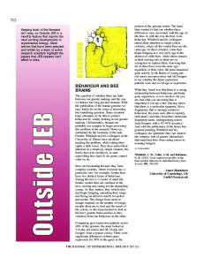
Figure 5: The performance of abnormality detection measured by detection rate and false alarm rate. (a)–(d) show the mean and ±1 standard deviation of the ROC curves obtained over 20 trials under different experimental settings.

mal if there were similar patterns that have been seen before and abnormal otherwise. The performance of the model is measured using the detection rate and false alarm rate in abnormality detection which are functions of T hΛ . Varying T hΛ gave us a ROC curve in each trial. The averaged ROC curves for N = 20 and N = 60 are shown in Fig. 5(a) and (b) respectively. Comparing Fig. 5 (a) with (b), it is clear that better performance was obtained using larger initial training sets. This was expected due to: (1) the models were initialised poorly given small N because the spectral clustering algorithm used for model initialisation requires sufficient data samples; (2) Some commonly occurred behaviour patterns were not present in the initial training set. Therefore, when they were observed after model initialisation, it took time for the model to integrate the corresponding behaviour classes into Mn . Nevertheless, it is observed that even with small initial training sets, our models were able to discover all the normal behaviour classes and reach convergence when sufficient observations became available after model initialisation. The experiments thus demonstrated that our incremental learning model can cope with changes of visual context (in this case, abnormal behaviour patterns becoming normal). Comparative evaluation against batch-mode offline learning — We compared the performance of our incremental behaviour modelling algorithm with a batch-mode offline model as follows. Given N behaviour patterns, a behaviour models were built following the same procedure as model initialisation for incremental learning (see Section 2.1). N was set to either 20 or 60 in our experiments. The

remaining behaviour patterns ( 142 − N in total ) were used for testing with the model parameters fixed during testing and abnormality detection performed using LRT (see Section 2.2). The experiment was repeated for 20 times each for N = 20 and N = 60 respectively and in each trial a behaviour model was trained with a different random training set. The averaged ROC curves obtained using models trained in batch mode are shown in Fig. 5(c) and (d). Comparing Fig. 5(a)&(b) with Fig. 5(c)&(d), it is evident that the incrementally learned models are superior to those learned in batch mode. The performance of the batch-mode behaviour models with N = 20 was especially poor (see Fig. 5(c)). This was mainly due to the fact that these models cannot cope with the changes of visual context. It is also noted that the ROC curves obtained using our incrementally models exhibited smaller variations across different trials. This again can be explained by the model adaptation feature of our method which makes the model less sensitive to the choice of initial training data. Computational cost — After model initialisation, the computational cost for incremental learning is significantly lower compared to the offline batch-mode method since only one behaviour pattern is used to update one mixture component of Mn or Ma at each time (see Table 2). More importantly, since our algorithm is online, it can run in real time. computational cost(second per frame) incremental 0.025 batch-mode 0.165 Table 2: Comparing the computational cost of incremental learning with that of a batch-mode learning method. These were for Matlab implementations.

4. Conclusion We proposed a fully unsupervised approach for visual behaviour modelling and abnormality detection. Our approach differs from previous techniques in that our model is learned incrementally online given an initial small bootstrapping training set. Furthermore, our model adapts to changes in visual context over time therefore catering for the need to reclassify what may initially be considered as being abnormal to be normal over time, and vice versa. It has been demonstrated by our experiments that our incrementally learned behaviour models are superior to those learned in batch mode in terms of both performance in abnormality detection and computational efficiency.

References [1] J. Berger. Statistical decision theory and bayesian analysis. Springer-Verlag, 1995.

[2] O. Boiman and M. Irani. Detecting irregularities in images and in video. In ICCV, pages 462–469, 2005. [3] H. Buxton and S. Gong. Visual surveillance in a dynamic and uncertain world. Artificial Intelligence, 78:431–459, 1995. [4] A. Dempster, N. Laird, and D. Rubin. Maximum-likelihood from incomplete data via the EM algorithm. Journal of the Royal Statistical Society B, 39:1–38, 1977. [5] T. Duong, H. Bui, D. Phung, and S. Venkatesh. Activity recognition and abnormality detection with the switching hidden semi-markov model. In CVPR, pages 838–845, 2005. [6] Z. Ghahramani. Learning dynamic bayesian networks. In Adaptive Processing of Sequences and Data Structures. Lecture Notes in AI, pages 168–197, 1998. [7] S. Gong and T. Xiang. Recognition of group activities using dynamic probabilistic networks. In ICCV, pages 742–749, 2003. [8] R. Hamid, A. Johnson, S. Batta, A. Bobick, C. Isbell, and G. Coleman. Detection and explanation of anomalous activities: Representing activities as bags of event n-grams. In CVPR, pages 1031–1038, 2005. [9] L.R.Rabiner. A tutorial on hidden Markov models and selected applications in speech recognition. Proceedings of the IEEE, 77(2):257–286, 1989. [10] R. J. Morris and D. C. Hogg. Statistical models of object interaction. IJCV, 37(2):209–215, 2000. [11] R. Neal and G. Hinton. A view of the em algorithm that justifies incremental, sparse, and other variants. In M. I. Jordan, editor, Learning in Graphical Models. Kluwer, 1998. [12] J. Ng and S. Gong. Learning intrinsic video content using levenshtein distance in graph partition. In ECCV, pages 670– 684, 2002. [13] N. Oliver, B. Rosario, and A. Pentland. A bayesian computer vision system for modelling human interactions. PAMI, 22(8):831–843, August 2000. [14] C. Stauffer and W. Grimson. Learning patterns of activity using real-time tracking. PAMI, 22(8):747–758, August 2000. [15] J. Wilpon, L. Rabiner, C. Lee, and E. Goldman. Automatic recognition of keywords in unconstrained speech using hidden markov models. IEEE Trans. Acoustic, Speech and Signal Proc., pages 1870–1878, 1990. [16] T. Xiang and S. Gong. Activity based video content trajectory representation and segmentation. In BMVC, pages 177– 186, 2004. [17] T. Xiang and S. Gong. Video behaviour profiling and abnormality detection without manual labelling. In ICCV, pages 1238–1245, 2005. [18] S. Yu and J. Shi. Multiclass spectral clustering. In ICCV, pages 313–319, 2003. [19] D. Zhang, D. Gatica-Perez, S. Bengio, and I. McCowan. Semi-supervised adapted hmms for unusual event detection. In CVPR, pages 611–618, 2005. [20] H. Zhong, J. Shi, and M. Visontai. Detecting unusual activity in video. In CVPR, pages 819–826, 2004.