Pursuing it, with eager feet,. Until it joins some larger way. Where many paths and errands meet. And whither than? I cannot say. - J.R.R. Tolkien ...
University of Alberta
Modelling the Behaviour of a Reverse-Flow Catalytic Reactor for the Combustion of Lean Methane by
Stephen Salomons A thesis submitted to the Faculty of Graduate Studies and Research in partial fulfilment of the requirements for the degree of Master of Science in Chemical Engineering Department of Chemical and Materials Engineering Edmonton, Alberta, Canada Spring 2003
Abstract Emissions of methane to the atmosphere are deemed by many to pose environmental problems.
Conversion of methane to carbon dioxide through
combustion reduces greenhouse gasses and can provide a source of energy. Catalytic combustion is a viable option for oxidation of lean methane streams. Lean methane mixtures can be very difficult to oxidize due to the relative stability of methane, and high temperatures are usually required. One option for increasing reactor temperature is to use flow reversal to trap energy in the reactor. This thesis details the development, validation and use of a transient 2D model for a reverse flow catalytic reactor. It is demonstrated that a 2D model can show many dynamics in the system that cannot be accurately reproduced with a 1D model. The model is verified with experimental data using a pilot scale reactor. This research presents results from numerical simulations and experiments into the effects of operating parameters such as feed rate, methane concentration, and cycle time.
The Road goes ever on and on Down from the door where it began. Now far ahead the Road has gone, And I must follow, if I can, Pursuing it, with eager feet, Until it joins some larger way Where many paths and errands meet. And whither than? I cannot say.
-
J.R.R. Tolkien
Dedication I would like to dedicate this work to my parents, brother, sister, brother-inlaw, and my many friends. I would like to thank them for their love, patience and support.
Acknowledgements I would like to acknowledge the people, without whom, this work would not have been possible. Dr. R.E. Hayes: My MSc program supervisor, who has given a fantastic opportunity to learn and grow. Dr Hayes has supported my study financially, and has guided my academic path.
I really appreciate his time, patience, and
wisdom. Dr. Michel Poirier and Dr. Hristo Sapoundjiev, CANMET: Who where involved with the experimental portions of this work. I would like to thank them for their guidance, advice, our discussions, and their many hours in the laboratory.
CANMET has also supported this work
financially. COURSE: Who have financially supported this work. Joe Mmbaga, Sam Mukadi, R Litto, Amika Kushwaha, and Errol D’Sousa: Who helped deal with many problems, great and small, and who were a joy to work with everyday. The Department of Chemical Engineering, University of Alberta: Who has helped train me in becoming a better engineer and scientist. Bob Barton and Jack Gibeau: Who have helped with many computer issues, great and small. University of Alberta, Computer and Network Services, Research Support: Who provided much of the computing resources required to solve the numerical problems.
Table of Contents List of Tables List of Figures Nomenclature 1 Introduction ..................................................................................................... 1 1.1 Fugitive Methane Emissions.............................................................................. 1 1.2 Greenhouse Gas................................................................................................. 1 1.3 Worker Safety ..................................................................................................... 3 1.4 Fuel Efficiency and Thermal Energy Generation.............................................. 3 1.5 Flaring ................................................................................................................. 4 1.6 Catalytic Combustion......................................................................................... 5 1.7 Introduction to Reverse Flow ............................................................................ 6 1.8 The Inert Layer .................................................................................................. 11 1.9 Monolith Conductivity ...................................................................................... 12 1.10 Reactor Modelling........................................................................................... 13 1.11 Intermediate Heat and Gas Withdrawal ......................................................... 13 1.12 Project Objectives .......................................................................................... 14 1.13 Layout of the Thesis....................................................................................... 15
2 Experimental Work........................................................................................ 16 2.1 The Reactor....................................................................................................... 16 2.1.1 Internal Structure ......................................................................................................... 19 2.1.2 Inert Monolith ............................................................................................................... 19 2.1.3 Active Packed Bed....................................................................................................... 20 2.1.4 Central Section ............................................................................................................ 20
2.2 Gas Feed Sources ............................................................................................ 20 2.3 Data Acquisition System and Operator Control ............................................. 21 2.4 GC Analysis ...................................................................................................... 22 2.5 Thermocouples................................................................................................. 22 2.6 Definition of a Cycle ......................................................................................... 26 2.7 Safety Switches ................................................................................................ 26 2.8 Preheating the Reactor..................................................................................... 27
3 The Model ...................................................................................................... 28 3.1 Introduction....................................................................................................... 28 3.2 Introduction to the Model................................................................................. 29 3.3 Model Equations ............................................................................................... 31 3.4 Properties of the Fluid and Solid..................................................................... 33 3.5 Rate of Reaction and Effectiveness Factor..................................................... 36 3.6 Mass and Heat Transfer Coefficients .............................................................. 38 3.7 Pressure Drop................................................................................................... 44 3.8 Boundary Conditions ....................................................................................... 45 3.9 Initial Conditions............................................................................................... 46 3.10 Numerical Solution ......................................................................................... 47 3.11 Optimising the Mesh ...................................................................................... 49 3.11.1 Increasing the Rate of Convergence ......................................................................... 50 3.11.2 Optimising Grid Spacing ............................................................................................ 54 3.11.3 Optimising the Beta Stretching Factor....................................................................... 56 3.11.4 Optimising The Time Step Size ................................................................................. 56
3.12 Investigation CFRR3: Comparison of Simulation and Experimental Results ................................................................................................................................. 60
4 Results and Discussion................................................................................ 68 4.1 Typical Experimental Results .......................................................................... 68
4.2 Effect of Radial Gradients ................................................................................ 72 4.3 Dual Peaks ........................................................................................................ 84 4.4 Response of radial gradients in monolith to flow reversal ............................ 88 4.5 Investigation CFRR7: Reactor Response to a sudden change in Inlet concentration: ........................................................................................................ 94 4.6 Boundary Conditions ....................................................................................... 99 4.7 External Heat Transfer Coefficient ................................................................ 100 4.8 Radial and Axial mixing factors in the Open Central Section...................... 102 4.9 One-Dimensional Model vs. Two-Dimensional Model.................................. 102 4.9.1 Thermocouple Fluctuations ....................................................................................... 109
4.10 Investigation CFRR2: Comparison of Simulation and Experimental Results ............................................................................................................................... 110 4.10.1 Comparisons at the Thermocouple Level................................................................ 110
4.11 Effectiveness Factors and Mass-Transfer Limitations............................... 116 4.12 Model Sensitivity to Reaction Rate.............................................................. 118 4.13 Sensitivity to the Inert type .......................................................................... 121 4.13.1 Inert sections, stability, and switch time .................................................................. 124
4.14 Optimising Switching times ......................................................................... 124 4.15 Summary ....................................................................................................... 127
5 Summary and Conclusions ........................................................................ 129 5.1 Reverse Flow .................................................................................................. 129 5.2 Experiments .................................................................................................... 129 5.3 The Model........................................................................................................ 130
6 Future Work ................................................................................................. 131 6.1 Mass and Heat Transfer Correlations in the Model ...................................... 131 6.2 Metal Monoliths .............................................................................................. 131 6.3 Model Comparisons for Different Inert and Catalyst Section Parameters.. 131
6.4 Thermal Energy and Enthalpy ....................................................................... 132 6.5 Improving Reactor Efficiency ........................................................................ 132 6.6 Lower Autothermal Limit................................................................................ 132 6.7 Process Control .............................................................................................. 133 6.8 Other Applications.......................................................................................... 133 6.9 Other Inlet Conditions .................................................................................... 134 6.10 Improving the Mesh...................................................................................... 134
References...................................................................................................... 136 Appendix......................................................................................................... 141 Experiment and Simulation Labels ..................................................................... 142 Experimental Conditions of Relevant Experimental Runs................................. 143 Sample Parameter File ......................................................................................... 144
List of Tables Table 2-1: Properties of the Inert Monolith......................................................................19 Table 2-2: Properties of the Reactor Packing. .................................................................20 Table 3-1: Enthalpy of reaction coefficients for methane.................................................36 Table 3-2: SIM24 shows the difference in speed of convergence when varying the maximum number of fixed point iterations per coupling iteration. ......................54 Table 3-3: Comparison of Element Sizes in SIM21. .........................................................55 Table 3-4: Comparison of Time Step Sizes in SIM20. ......................................................57 Table 4-1: A comparison of fractional conversion after 5 full cycles using various preexponential kinetic factors. .................................................................................118
List of Figures Figure 1-1: A unidirectional flow reactor will show a temperature profile similar to the top forward flow profiles (a) and (b). In reverse flow, the flow direction is switched to accumulate energy in the centre of the reactor over progressive cycles as shown in (c), (d) and (e). []......................................................................8 Figure 1-2: The reverse-flow reactor concept. For a determined length of time, the reactor will run in forward flow, indicated by the dark blue arrows. After a determined amount of time, the flow direction will be changed to reverse flow, as indicated by the light red arrows. Surrounding the reactor is a layer of insulation. The open central section may be used for heat or gas extraction. In the experiments presented in this thesis, no heat or gas extraction is used..........10 Figure 2-1: Diagram of the reactor and associated piping. Thermocouple locations are also shown.............................................................................................................17 Figure 2-2: Schematic of the reactor, including valves, thermocouples, and thermocouple locations. Radial thermocouple locations are shown in the circles. The heat exchanger and gas withdrawal set-up is also shown............................................18 Figure 2-3: The locations of the centreline thermocouples on a dimensionless scale. ....24 Figure 2-4: A photograph of the top of the monolith section, showing the radial placement of the thermocouples............................................................................25 Figure 3-1: The mesh used to solve the differential equations. The figure on the left is the entire mesh, and the figure on the right is a zoomed in picture of the mesh at the interface between the inert and the catalyst....................................................51 Figure 3-2: Optimisation of the grid, using various radial spacing. After simulating a 250-second half-cycle, the differences between the smoothness of the temperature gradients at different radial spacings may be shown. ..........................................52 Figure 3-3: The same data as shown in Figure 3-2, except that the mesh lines are removed from view to allow easier viewing of the irregularities in the solution on the coarser grids. The temperature contour map is in units of (K). ....................53 Figure 3-4: A comparison of the sum of the number of coupling iterations required over a half-cycle in SIM20 for various step sizes. Note that for larger step sizes, although few time steps are required, more coupling iterations are required per time step. The best balance to minimise the number of coupling iterations (and thus the execution time) while maintaining high accuracy and usability appears to occur when the time step size is one (1) second................................................59
Figure 3-5: Comparing the predictions of SIM3 with experimental results (EXP3). The inlet conditions are 0.21 m/s feed with 0.89% v/v methane (at ambient conditions). The cycle times are not constant. In this graph, we are looking at the data after 1140 time steps. This is the end of the third full cycle, which had a full cycle length of 360 seconds. Cycle one was 420 seconds in length, and cycle two was 360 seconds in length. The simulation concentration profile that corresponds to this data is in Figure 4-12. The dots are experimental results, and the line is the simulation result. ............................................................................61 Figure 3-6: Similar conditions to Figure 3-5, but after 1260 time steps..........................62 Figure 3-7: Similar to Figure 3-5, but after 1380 time steps. ..........................................63 Figure 3-8: Similar to Figure 3-5, but after 1560 time steps. ..........................................64 Figure 3-9: Two dimensional temperature representation of Figure 3-7 (1380 time steps). This data is from the simulation. Radial gradients within the active catalyst are very visible in the plot. The centreline is r = 0. ...............................66 Figure 3-10: Two dimensional temperature representation of Figure 3-8 (1560 time steps). This data is from the simulation. Radial gradients within the active catalyst are very visible in the plot. The centreline is r = 0. ...............................67 Figure 4-1: Typical axial temperature profiles obtained during autothermal operation at 0.34 m/s inlet velocity and 0.22% methane (EXP31). Cycles were 600 seconds in length. The profiles are shown at the end of the reverse flow half-cycle, that is, with flow from the left section to the right section................................................70 Figure 4-2: Axial temperature profiles obtained for a single cycle at two different methane inlet concentrations and a common inlet velocity of 0.34 m/s. The symmetric cycles were 600 seconds long. For each case the profile at the end of the forward flow (right to left) and reverse flow (left to right) half-cycles are shown. EXP31 has an inlet concentration of 0.22% CH4, and EXP32 has an inlet concentration of 0.34%. ........................................................................................71 Figure 4-3: Radial gradients experimentally observed in the left side monolith inert section. This graph shows the progression of the gradient starting at the beginning of cycle 19, and ending one full cycle later at the start of cycle 20. Cycle time in this experiment was 600 seconds for a full cycle. Inlet conditions included an inlet concentration of 0.22% methane at a feed gas superficial velocity of 0.34 m/s (50.3 kg/h) at ambient conditions. The data is from EXP31. ...............................................................................................................................73 Figure 4-4: Radial gradients experimentally observed in the right side monolith inert section. This graph shows the progression of the gradient starting at the beginning of cycle 19, and ending one full cycle later at the start of cycle 20. Cycle time in this experiment was 600 seconds for a full cycle. Inlet conditions
included an inlet concentration of 0.22% methane at a feed gas superficial velocity of 0.34 m/s (50.3 kg/h) at ambient conditions. The data is from EXP31.74 Figure 4-5: Thermocouple recordings experimentally that are observed in the left side catalyst packed bed section. This graph shows the progression of the thermocouples over three full cycles. Cycle time in this experiment was 600 seconds for a full cycle. Inlet conditions included an inlet concentration of 0.22% methane at a feed gas superficial velocity of 0.34 m/s (50.3 kg/h) at ambient conditions. The data is from EXP31. ....................................................................75 Figure 4-6: Thermocouple recordings experimentally that are observed in the right side catalyst packed bed section. This graph shows the progression of the thermocouples over three full cycles. Cycle time in this experiment was 600 seconds for a full cycle. Inlet conditions included an inlet concentration of 0.22% methane at a feed gas superficial velocity of 0.34 m/s (50.3 kg/h) at ambient conditions. The data is from EXP31. ....................................................................76 Figure 4-7: Same data set as Figure 4-6, but over many more cycles. The data is from EXP31. ..................................................................................................................77 Figure 4-8: Thermocouple progression in the left monolith over three full cycles in investigation CFRR7. The data is from EXP7. The inlet velocity was 0.68 m/s (ambient conditions) and inlet concentration was 0.33% methane. Full cycles were 400 seconds in length. ..................................................................................79 Figure 4-9: Thermocouple progression in right monolith over three full cycles. The data is from EXP7. The inlet velocity was 0.68 m/s (ambient conditions) and inlet concentration was 0.33% methane. Full cycles were 400 seconds in length. .....80 Figure 4-10: The observation of dual peaks in an experiment (CFRR8) using 0.18 m/s feed gas (under ambient conditions), 1.25% methane, and asymmetric half-cycles. This profile is from the time step 1200 seconds into the experiment. ...................85 Figure 4-11: The observation of dual peaks in an experiment (CFRR8) using 0.18 m/s feed gas (under ambient conditions), 1.25% methane, and asymmetric half-cycles. This profile is from the time step 1440 seconds into the experiment, or 240 seconds after the profile expressed in Figure 4-10...............................................86 Figure 4-12: Profile of the methane fraction along the centreline and beside the reactor wall, as per simulation. Most of the conversion here occurs in the first reactor section encountered. The corresponding temperature profile is in Figure 3-5. This data is from SIM3..........................................................................................89 Figure 4-13: Thermocouple progression in left catalyst over three full cycles, as measured in EXP7. The inlet velocity was 0.68 m/s (ambient conditions) and inlet concentration was 0.33% methane. Full cycles were 400 seconds in length. ...............................................................................................................................92
Figure 4-14: Thermocouple progression in right monolith over three full cycles, as measured in EXP7. The inlet velocity was 0.68 m/s (ambient conditions) and inlet concentration was 0.33% methane. Full cycles were 400 seconds in length. ...............................................................................................................................93 Figure 4-15: The response of the left reactor to an instant kill of the methane feed. Initially, 0.68 m/s of gas with 0.33% methane is being fed to the reactor. At cycle 3, the methane feed is discontinued (leaving 0.68 m/s of gas at 0% methane). After one full cycle, the feed is restored to 0.33% methane. Full cycles are 400 seconds in length. Shown is the response of the left side reactor. ........................95 Figure 4-16: The response of the reactor to an instant kill of the methane feed. Initially, 0.68 m/s of gas with 0.33% methane is being fed to the reactor. At cycle 3, the methane feed is discontinued (leaving 0.68 m/s of gas at 0% methane). After one full cycle, the feed is restored to 0.33% methane. Full cycles are 400 seconds in length. Shown is the response of the right side reactor. .......................................96 Figure 4-17: The response of the reactor to an instant kill of the methane feed in Investigation CFRR7. Initially, the profile is relatively high. The inlet methane concentration is reduced to zero at the beginning of cycle 3, and the reactor looses thermal energy. At the beginning of cycle 4 the methane is restored, and the reactor slowly recovers thermal energy. These profiles show the centreline profiles at the beginning of the stated cycles. .......................................................97 Figure 4-18: Similar to Figure 4-17, but at the end of the half cycle...............................98 Figure 4-19: A comparison of the external heat transfer coefficients used in simulations SIM2, SIM21 and SIM22 at time step 2250. Note that the centreline and wall profiles for all three simulations appear lined up, with no significant difference. .............................................................................................................................101 Figure 4-20: A comparison of 1-D and 2-D simulations to experimental data. Full cycles are 500 seconds in length. Inlet methane concentration is 0.39% and inlet superficial velocity is 0.42 m/s (both at ambient temperature and pressure). This graph shows the centreline profiles from SIM1 and SIM2 and the experimental data points along the centreline. This is the profile after the first half cycle. ...104 Figure 4-21: Same conditions as for Figure 4-20, but after 500 seconds (at the end of one full cycle). .....................................................................................................105 Figure 4-22: Same conditions as Figure 4-20, but after 2750 seconds (after five and a half full cycles). ...................................................................................................106 Figure 4-23: Same conditions as Figure 4-20, but after 3000 seconds (at the end of six full cycles). ..........................................................................................................107 Figure 4-24: A comparison between the experimentally obtained data at the thermocouple K (left reactor) and the simulation data at the point where the same
thermocouple was said to be in the mesh. The simulation appears to be showing a slightly higher prediction that experimentally observed in this case...............112 Figure 4-25: A comparison between the experimentally obtained data at the thermocouple L (left reactor) and the simulation data at the point where the same thermocouple was said to be in the mesh. Initially, the simulation appears is way off. However, towards the end of the simulation, the agreement is better.........113 Figure 4-26: A comparison between the experimentally obtained data at the thermocouple K (right reactor) and the simulation data at the point where the same thermocouple was said to be in the mesh. The simulation is not predicting the same behaviour at this single point in the reactor........................................114 Figure 4-27: A comparison between the experimentally obtained data at the thermocouple T (right reactor) and the simulation data at the point where the same thermocouple was said to be in the mesh. The simulation appears to be predicting the experimental data fairly well in this case. ...................................115 Figure 4-28: The effectiveness factors and Thiele Modulus for the reaction and reactor under study. Typical operation of the reactor is between 700-1300 K (Thiele Modulus of 100-700). The effectiveness factor in this range is between 0.03 and 0.004....................................................................................................................117 Figure 4-29: The initial conditions used for SIM10, SIM11, and SIM12.......................119 Figure 4-30: Fractional conversion over a progression of cycles at various reaction rate pre-exponential factors. Note: The reactor geometry in this simulation is not the same as the reactor geometry in the experiments. ..............................................120
Nomenclature Where the variables are defined as: 1 1radial 1axial 1i ε 2 3 ρf ρs 4 τ φ 56
= Thermal diffusivity, m2 s = Thermal diffusivity, radial component, m2 s = Thermal diffusivity, axial component, m2 s = Stoichiometric coefficient of component i = Porosity, dimensionless = Effectiveness factor, dimensionless = Fluid viscosity, N s m-2 = Density of the fluid, kg m-3 = Density of the solid, kg m-3 = Thiele modulus, dimensionless = Tortuosity of a pore in the parallel pore model, dimensionless = Fraction of gas withdrawn, dimensionless = Atomic diffusion volume for use with Fuller equation, dimensionless
av a
= Area per volume, m2 m-3 = Power coefficient for rate dependence on CH4, dimensionless
b B
= Power coefficient for rate dependence on O2, dimensionless = Parameter in Dixon and Creswell packed bed model, dimensionless
C c Cp,a,i Cp,b,i Cp,c,i Cp,d,i Cp,bar Cp,f Cp,s
= Total molar concentration, mol m-3 = Power coefficient for rate dependence on adsorption, dimensionless = First heat capacity coefficient for fluid component i, J kg-1 K-1 = Second heat capacity coefficient for fluid component i, J kg-1 K-2 = Third heat capacity coefficient for fluid component i, J kg-1 K-3 = Fourth heat capacity coefficient for fluid component i, J kg-1 K-4 = Heat capacity of the fluid mixture, J kg-1 K-1 = Heat capacity of the fluid, J kg-1 K-1 = Heat capacity of the solid, J kg-1 K-1
Da DA DA,B Dchannel Dchar,packing Dchar
= Damköhler number, dimensionless = Bulk diffusion coefficient, m2 s-1 = Diffusion coefficient of component A in component B, m2 s-1 = Monolith channel diameter, m = Characteristic diameter of the packing, m = Characteristic diameter, m
Deff Dh DI,z DI,r Dk
= Effective diffusivity, m2 s-1 = Hydraulic diameter, m = Dispersion term, axial component, m2 s-1 = Dispersion term, radial component, m2 s-1 = Knudsen diffusion, m2 s-1
EA Ea,1 Eb,1
= Activation energy of reaction, J mol-1 = Activation energy of adsorption of CH4, J mol-1 = Activation energy of adsorption of O2, J mol-1
G Gz
= Effective radial thermal conductivity factor in a monolith, dimensionless = Graetz number, dimensionless
h hm 7Hform 7Hrxn
= Heat transfer coefficient, W m-2 K-1 = Mass transfer coefficient, m s-1 = Heat of formation, J mol-1 = Heat of reaction, J mol-1
k ka kax,eff krad,eff kb kz,f kr,f kf kg,i kw
= Overall reaction rate constant, s-1 = Rate constant for adsorption of CH4, dimensionless = Effective axial thermal conductivity, W m-1 K-1 = Effective radial thermal conductivity, W m-1 K-1 = Rate constant for adsorption of O2, dimensionless = Effective axial thermal conductivity of the fluid, W m-1 K-1 = Effective radial thermal conductivity of the fluid, W m-1 K-1 = Thermal conductivity of the fluid, W m-1 K-1 = Mass transfer coefficient, m s-1 = Thermal conductivity of the solid, W m-1 K-1
M MA MB
= Average molar mass of gas components, g mol-1 = Molar mass of component A, g mol-1 = Molar mass of component B, g mol-1
Nu NuT
= Nusselt number, dimensionless = Nusselt number for constant wall temperature case, dimensionless = Nusselt number for constant heat flux case, dimensionless
NuH OFA
= Fractional open frontal area (or porosity) of a monolith, dimensionless
P Pe Peax Perad
= Pressure, Pa = Peclet number, dimensionless = Peclet number, axial component, dimensionless = Peclet number, radial component, dimensionless
Pr
= Prandtl number, dimensionless
r R Ri(CS,TS) Re
= Radial coordinate, m = Ideal gas constant, J mol-1 K-1 = Rate of reaction in the catalyst, mol m-3 s-1 = Reynolds number, dimensionless
Sc Sh ShH ShH1
= Schmidt number, dimensionless = Sherwood number, dimensionless = Sherwood number, constant heat flux case, dimensionless = First shape constant for Sherwood number, constant heat flux case, dimensionless = Second shape constant for Sherwood number, constant heat flux case, dimensionless = Sherwood number, constant wall temperature case, dimensionless = First shape constant for Sherwood number, constant wall temperature case, dimensionless = Second shape constant for Sherwood number, constant wall temperature case, dimensionless
ShH2 ShT ShT1 ShT2 t Tf Ts twc
= Time, s = Temperature of the fluid, K = Temperature of the solid, K = Thickness of the washcoat, m
YCH4 Yi Yf Yi,f YO2 Ys
= Molar fraction CH4, dimensionless = Molar fraction of component i, dimensionless = Molar fraction in the fluid phase, molar fraction = Molar fraction of component i in the fluid phase, dimensionless = Molar fraction O2, dimensionless = Molar fraction in the solid phase, molar fraction
v
= Fluid velocity, m s-1
z zentry length
= Axial coordinate, m = Entry length, m
1 Introduction
1.1 Fugitive Methane Emi ssions Emissions of methane to the atmosphere are deemed by many to pose environmental problems.
Global warming is thought to be accelerated by
increased methane levels. These methane emissions come from a variety of sources. In 1999, Canada emitted an estimated 4300 kilotons of methane, of which 1800 kilotons (42%) was attributed to fugitive emissions in the oil and gas sector, and 51 kilotons (1%) to fugitive emissions in the solid fuels and coal mining sector [1]. Agricultural emissions accounted for 1100 kilotons or 26% of total methane emissions. Most fugitive emissions (from human activity) come from leaks during the extraction, processing and transporting of oil and gas [2]. For example, gasses are dissolved in oil reserves.
In the process of extracting petroleum, the
dissolved gas is brought to the surface with the liquid oil. For low flowrate oil wells, the gas is often vented to the atmosphere, as collection is considered uneconomic. Fugitive emissions are a source of many varied problems in the industrial world. Accumulation of fugitive emissions in a small-enclosed space may create a potentially explosive atmosphere.
Large-scale accumulation of fugitive
emissions is thought to affect global climate change.
By minimizing fugitive
emissions, the risks and problems associated with these gasses may be diminished.
1.2 Greenhouse Gas Global warming is a major issue in the world today. It has been suggested that excessive levels of greenhouse gas (GHG) in the atmosphere influence
1
climate change. Methane is classified as a GHG, and large volumes of methane in the atmosphere are suggested to be contributing to climate changes today. On April 29, 1998, Canada signed [3] the Kyoto Protocol [4], and committed to minimizing GHG emissions. The combined effort of the industrial world will be required to reach the goals set out by the Kyoto Protocol. Under Article 2.1.a.viii of the protocol, methane is classified as a GHG. GHG emissions are usually reported in terms of equivalent carbon dioxide emissions. Canada's goal under Annex B of the Kyoto Protocol is to reduce aggregate anthropogenic carbon dioxide equivalent emissions of the greenhouse gasses to 94% of our level in the base year (1990) by the target date in Article 3.1 of 2008-2012. Methane is listed as a GHG in Annex A of the protocol, and has a global warming potential 21 to 23 times that of carbon dioxide [2,5,6,7]. Methane is also one of the most common of the six greenhouse gasses. In 1999, Canada's GHG emissions [1] included 44 000 kilotons of equivalent carbon dioxide from fugitive emissions in the energy industry.
Methane
emissions through agricultural activities are responsible for 23 000 equivalent kilotons, and solid waste is responsible for approximately 22 000 kilotons. In total, Canada is estimated to have emitted 699 000 equivalent kilotons of carbon dioxide in the year 1999. Approximately 13%, or 90 000 equivalent kilotons of carbon dioxide, involves methane emission. Reducing methane emissions will have a strong impact on equivalent carbon dioxide emissions. The importance of finding and utilizing efficient methods of reducing equivalent carbon dioxide emissions through reducing methane emissions is apparent. In the complete combustion of methane to carbon dioxide, methane and carbon dioxide balance 1:1 in a molar ratio.
CH 4 +2O2 → CO2 +2H 2O
(1.1)
However, because methane has 21 to 23 times the global warming potential as carbon dioxide, the complete combustion of methane will reduce equivalent carbon dioxide emissions by approximately an order of magnitude on a mass basis.
2
1.3 Worker Safety Another motivation for reducing fugitive methane emissions is worker safety.
Coals mines and oil drill sites are known for their harsh conditions.
Recent mine explosions in the Westray Mine in Nova Scotia [8], Ukraine [9,10], China [11] and others [12,13], have cost many miners their lives. Lean methane is commonly present in a mine atmosphere, and may become very dangerous when it accumulates up to the lower explosive limit [14], 5% by volume in air. Ensuring that mineshaft methane levels are at safe levels is critical to worker safety. Because methane is present in the ground and released by mining and drilling activities, the methane must be vented and the mine atmosphere cleaned and refreshed.
1.4 Fuel Efficiency and Th ermal Energy Generation Methane can be a useful gas. If the gas can be captured, it can be used as a fuel to provide utility energy. An additional motivation for burning lean methane sources is to maximise the efficiency and utility of an energy source. High concentrations of methane may be burned in a simple manner, producing thermal energy, which may be used as a heat source or converted into electricity. Lean methane may also undergo combustion to produce a utility heat source under more specific circumstances. Most often, lean methane emissions are simply considered waste gas, and vented. However, this gas may be a useful energy source. Every tonne of emitted methane may be considered to be a tonne of wasted fuel and lost utility. If the energy in this gas can be captured and used to supplement current energy sources, then perhaps a site’s overall fuel consumption can be reduced, thus lowering operating costs.
3
1.5 Flaring Many methods of dealing with fugitive emissions have been used over the years. Flaring of fugitives at a wellsite is a cheap way of dealing with them, but the method has a social stigma attached to it, making project approval more time consuming. When drilling for oil, various gasses stored in the ground and dissolved in the oil below are disturbed and seep out. Not all of these gasses are intended for production, but are present nonetheless. These gasses must be dealt with before they reach hazardous levels, and are often burnt in a flare. Flares are relatively cheap to build, and simple to operate. In most cases, flares are used to combust the hazardous gasses into another gas that is less dangerous. However, unless the fuel and flame conditions are carefully monitored, harmful side reactions (such as the conversion of N2 to NOx) may result. Flares introduce problems when attempting to obtain project approval by a public office.
Owing to the environmental issues surrounding flares, public
opposition to flares often makes project approval by government agencies more difficult, delaying project timelines, and adding to overall costs. There is also speculation that flaring produces byproducts that increase the local rate of cancer [15,16]. Also, for direct flaring to work, the concentration of the feed methane must be above approximately 5%. Below this concentration, flaring is not a viable option. The concentration of ambient methane in coal mines and in fugitive emissions is typically very low (0.3 – 1.0% v/v).
Simple homogeneous
combustion reactions are unfavorable at such low to moderate concentrations. Thermal incineration (homogeneous combustion) is another method that could potentially be employed, however it requires the addition of a support fuel. The additional support fuel adds to higher operating costs. This may not be a viable option at remote drill sites or deep in mines. Also, the high temperatures associated with thermal incineration increase the probability of forming significant levels of NOx in the process. NOx is another pollutant whose production should be avoided, as it is a major contributor to smog [2]. Legislated limits are placed 4
on the release of NOx.
1.6 Catalytic Combustion One method of burning lean methane and reducing equivalent carbon dioxide emissions is through the use of flameless catalytic combustion. This is a heterogeneous process, which may occur on both noble and non-noble metal catalysts. This was perhaps first observed by Sir Humphry Davy in 1818 [17], while studying safety lamps in the lean-methane atmosphere found in coal mines.
Davy found that oxygen and coal gas (methane) reacted on a hot
platinum wire without a flame, but produced enough heat for the reaction to be sustainable. The heterogeneous process of flameless catalytic combustion over either noble or non-noble metal catalysts has shown to be effective [18-25], even at low concentrations.
Several different metals have been used as catalysts.
Platinum [18] and palladium [19,20,21,22,23] are perhaps the most common for methane combustion.
Sapundzhiev et al. [24] and Cimino et al. [25] used
perovskite-based catalysts for autothermal combustion of lean methane mixtures. During catalytic combustion, oxidation may also occur homogeneously; however, the homogeneous process is much slower kinetically than the heterogeneous process. At relatively lower temperatures (below 1000ºC), the homogeneous process is not significant, compared to the reaction rate of the heterogeneous process.
Veser and Frauhammer [18] found that the
homogeneous oxidation of methane may be neglected. They found that rate of surface adsorption of methane is much higher than the rate of homogeneous reaction even at temperatures up to 1200ºC. Catalytic combustion reactors have been studied for a number of years [17,26,27,28], especially in the form of automotive catalytic converters. However, the detailed transient study of large scale catalytic combustion reactors is more recent.
5
A typical feed stream of lean methane from fugitive sources is at ambient temperatures.
At such relatively low temperatures, the heterogeneous
combustion reaction is exceptionally slow. The reaction proceeds at a much higher rate and at greater efficiency at much higher temperatures. However, in order for an ambient feed stream to react at higher temperatures, that feed stream must somehow be preheated before the reaction takes place. This is difficult to do efficiently. There are several methods that can be used to preheat the inlet ambient feed to a higher (and more efficient) temperature. If the feed is heated using an external heat source before the reaction inlet, there is the additional cost of powering the external heater. Another method is to run the hot outlet feed gas through a heat exchanger to preheat the feed.
While this may not require
external thermal energy, there is an added pressure drop associated with a heat exchanger that has excellent heat transfer and mixing properties.
Another
method is to use the thermal mass within the reactor to store and transfer thermal energy, while switching the direction of flow in a manner that efficiently preheats the feed with the energy of combustion.
1.7 Introduction to Revers e Flow Typical reactors, such as the fixed bed type often found in industry, are operated in a unidirectional manner. There is a fixed inlet and a fixed outlet. A reverse-flow reactor does not have a fixed inlet or outlet. The inlet is periodically switched between two sides of a reactor. Thermal energy generated in an exothermic reaction in a well-insulated unidirectional reactor is often lost to the outlet stream.
Reverse-flow, a forced
unsteady state process, is used to help utilise the thermal energy inside a reactor. Energy from the reaction and exit gasses are captured and utilised within the reactor by the reversing flow action. The captured thermal energy can be used to preheat the feed or extracted from the reactor. This allows a reactor core to remain at high temperatures, even if the inlet feed is at lower, ambient
6
temperatures. A unidirectional flow reactor would show a temperature profile over time similar to that shown in Figure 1-1 a and b. The concept of reverse flow was first discussed by D.A. Frank-Kamenetski in 1942 and published in his book in 1955 [29].
However, at the time, the
concept was not feasible. Early issues with oscillations and dealing with the accumulation of thermal energy discouraged the technology at the time. Significant improvements have been made [27] in catalyst and reactor technology since then and the technology is now practical. The concept has been used in many applications, many of which have been reviewed by Matros and Bunimovich [27]. These applications include VOC oxidation reactions, the partial oxidation of natural gas, selective catalytic reduction of NOx by ammonia, and SO2 oxidation in sulfuric acid production. The adaptation of reverse-flow to the combustion of lean methane mixtures is relatively new. With reverse flow, reactions that are not normally autothermal may be run and sustained at lower inlet temperatures and higher conversions than possible in a direct flow adiabatic reactor. A reverse-flow reactor may need some initial preheating to bring the catalyst to an acceptable temperature, but a welldesigned reactor should be able to thermally sustain itself once running. Liu [30] has done extensive research into the use of a reverse flow catalytic converter in an automobile application. If similar equipment were used, but in unidirectional mode, the reaction typically would self-extinguish. As more feed gas enters the reactor and is preheated by the inlet inert section, the thermal energy stored in the inert section is depleted. Soon, the catalyst section begins to be cooled by the incoming gas and the reaction rate lowers. extinguished itself very quickly.
7
The reactor will have
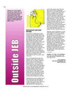
Figure 1-1: A unidirectional flow reactor will show a temperature profile similar to the top forward flow profiles (a) and (b). In reverse flow, the flow direction is switched to accumulate energy in the centre of the reactor over progressive cycles as shown in (c), (d) and (e). [31]
8
The thermal energy generated by an exothermic reaction may be captured and stored in the solid material in a reactor where it can be used to maintain a high reaction temperature. The reactor may be run as a traditional fixed-bed reactor if desired. A packed bed, monolith or other section may be used in the active section of the reactor. Typically, there is also an inert section (either a monolith or packed bed) on either side of the catalyst section that is used to help store thermal energy from the heat of reaction and transfer that heat to inlet gas as a means of preheating the feed gas.
As time progresses, more energy
accumulates at the outlet of the reactor. After a determined length of time, the flow direction is reversed, and the thermal energy stored in the inert sections is used to preheat the feed. This time is typically before the reactor begins to lose thermal energy. When the flow direction is reversed, the temperature profile continues in Figure 1-1 from a and b to c and d. Again, after a determined amount of time, the direction is switched. Figure 1-2 shows the two different flow directions in reverse flow.
9
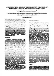
Figure 1-2: The reverse-flow reactor concept. For a determined length of time, the reactor will run in forward flow, indicated by the dark blue arrows. After a determined amount of time, the flow direction will be changed to reverse flow, as indicated by the light red arrows. Surrounding the reactor is a layer of insulation. The open central section may be used for heat or gas extraction. In the experiments presented in this thesis, no heat or gas extraction is used.
10
1.8 The Inert Layer Sapundzhiev et al. [32] were among the first to report the use of an inert layer at the entrance and exit of the reactor to retain heat and minimise the amount of active catalyst required. Hot exit gas from the reactor heats up the exit inert layer, storing thermal energy. Thus when the flow direction is reversed, the warm inert section now uses this stored thermal energy to preheat the feed. Figure 1-1 shows this thermal progression. When the feed gas encounters the catalyst sections, it has already warmed up from the inlet temperature. The gas may now react at a slightly higher temperature, and with a slightly higher conversion, than if there was no preheat. The exit inert section on the other side now gains stored thermal energy during this phase of the cycle. After a time period, the flow direction is again reversed, with the stored thermal energy in the new entrance inert section preheating the feed. As this cycle continues, the total amount of thermal energy stored in the reactor slowly increases until a pseudosteady state regime is attained. Periodic flow reversal may be used to accumulate heat within the reactor, allowing for reactions to take place at a higher temperature than would otherwise be allowed in a classic catalytic reactor [24].
As the outer sections tend to be cooler and have a less significant
contribution to the reaction kinetics, these outer sections may be replaced with inert material. Inert material may have similar heat transfer properties as the catalyst, but may be many times cheaper to manufacture. The inert sections allow a reactor to be designed using less catalyst, lowering the overall capital investment in such a reactor. The configurations of the inert and catalyst sections of a reactor are of the designers’ choice.
They may be structured monoliths [33], packed beds (of
spheres, Raschig rings, Berl saddles or others), or any other standard packing type. An advantage of using a monolith in lieu of a packed bed is the much lower pressure drops associated with the monoliths.
11
Groppi and Tronconi [34]
reported pressure drops of 0.5% of inlet pressure, or up to two orders of magnitude lower than a conventional packed bed. Poirier et al. [35] reported a ceramic monolith pressure drop that was one tenth of the pressure drop of an equivalent Denstone ball inert section. Lower operating costs may be realised as a result of a lower pressure drop. The heat transfer properties of a monolith will differ from those of a packed bed. There must be a balance between heat transfer, low pressure drop, and adequate mixing. The optimal size monolith is not yet clear.
1.9 Monolith Conductivity Groppi and Tronconi [23] considered the design of monolith catalysts that allow high conversion and minimise temperature gradients while reducing the pressure drop. They discuss [36] using the thermal conduction properties of the monolith support as an additional thermal energy (heat) transfer mechanism. The effective thermal conductivities of a monolith support are directly proportional to the intrinsic conductivity. Thus, one should choose a material with a relatively large thermal conductivity when designing a reactor.
They
suggest that the optimal structure may include a high intrinsic conductivity, and that metallic monoliths may prove to be useful in providing this property. The high intrinsic thermal conductivity is expected to allow greater heat conduction, allowing thermal energy to redistribute itself more evenly across the monolith section. From their simulation results, the highly conductive monolith with appropriately chosen volume fraction variables approaches virtually isothermal operation at high conductivities (ks ~= 200 W·m-1·K-1). This spreads out the thermal energy in a more even fashion, and may help to keep the reactor stable and increase overall conversion by reducing localised peaks. Groppi and Tronconi identified two issues that may arise from the use of highly conductive monoliths.
The first issue is that the controlling thermal
resistance in the radial direction may become the contact resistance between the
12
monolith and the reactor wall. Attention must then be paid to the monolith/wall interface to optimise that contact resistance to a value best suited to the reaction and application. The second issue is with regard to the degree of loading of the catalyst on the monolith. The monoliths used in Groppi and Tronconi’s study appear to have a much lower catalyst loading than typical packed beds, which may limit the reactor’s specific productivity. Groppi and Tronconi make several suggestions that may eliminate this problem, but more research must be done to properly investigate the effects of each suggestion.
1.10 Reactor Modelling Owing to the difficulty in comparing different sets of experimental results and the expense associated with building a new pilot plant reactor, studies may be more efficiently performed using a computer model. The cost and time that is required to manufacture new components, inserts, or a reactor with untested dimensions is relatively high. Testing new inserts or a reactor of new dimensions in a computer model is much simpler and much more cost-effective. Potential designs may be evaluated in the simulation to determine the best design to build for a specific application. However, before a model may be considered to be useful, the model must first be verified and calibrated using experimental results.
1.11 Intermediate Heat and Gas Withdrawal Intermediate heat removal is very useful in the operation of a reverse-flow reactor. This is where the energy is extracted from the reactor, and made available as a utility heat source. Heat removal may be usually accomplished by use of one or more heat exchangers or through gas withdraws in the reactor centre. Also, intermediate heat withdraw may help ensure the stability of the reactor by ensuring that a reactor does not indefinitely accumulate thermal
13
energy and rise in temperature, to the detriment of the catalyst and solid materials. If the temperature in the reactor gets too high, the heat exchanger may be used to extract excess thermal energy, and keep the reactor within an acceptable temperature range. There is a disadvantage to utilizing a heat exchanger for thermal energy extraction.
Any new equipment added to a reactor will have an associated
pressure drop.
The addition of a heat exchanger will increase the overall
pressure drop significantly. A gas withdrawal system may have a much less significant effect on pressure drop, as the system is less obtrusive to the gas flow. However, the change in flowrate in the second half of the reactor must be considered. The superficial velocity of the gas in the second half of the reactor is lowered slightly by the withdrawal of a significant portion of the stream. This may slightly increase the residence time of the reactants that are present in the second reactor, and slightly increase the fractional conversion of that stream. The system used in the experiments presented in the thesis is designed to be run with intermediate gas withdrawal. The hot gas that has been withdrawn is passed though a heat exchanger to recover the heat.
However, in the
experiments and simulations to be presented, no gas withdrawal is used. Research in that area will be conducted in the future.
1.12 Project Objectives The objective of this study was to develop and evaluate a computer model for evaluating the performance of a transient reverse-flow reactor system for the combustion of lean methane, and to investigate reactor performance using monolith inserts.
The reactor had both monolith and packed bed sections.
Experimental results over a methane concentration range of 0.2 to 1.25%, a superficial inlet velocity range of 0.18 to 0.76 m/s, and a (full) cycle time range of 400 – 800 seconds were obtained. An evaluation of the use of a monolith section instead of a traditional packed bed for the inert section is attempted.
14
1.13 Layout of the Thesis Background to the basic concepts of catalytic combustion and reverse flow are presented in chapter 1. Chapter 2 outlines the experimental apparatus used and the work performed, and some of the experimental procedures. development of the mathematical model is described.
In chapter 3, the
Reasoning for various
choices and assumptions in developing the model are given.
The computer
model and the choices of various modeling parameters are also discussed. Results and discussion are found in chapter 4. This chapter compares the experimental results with the simulation predictions and validates the model. Observations from the experimental work are presented. Conclusions and future work possibilities are discussed in chapters 5 and 6, respectively.
15
2 Experimental Work
Experimental work was performed with the generous co-operation of Natural Resources Canada - CANMET Energy Technology Centre Varennes in Varennes, Quebec, Canada.
2.1 The Reactor A reverse-flow reactor with an inner diameter of 200 mm was used for the experimental work. Two reaction sections stand beside each other, connected at the bottom by a U-shaped pipe.
An overview of the reactor, highlighting
important parts, is given in Figure 2-1, and a more complete schematic is shown in Figure 2-2. The reactor walls are made of Hastelloy, a high strength, nickel-based alloy, to allow operation at temperatures up to approximately 1000 °C. However, operation above ~ 900 °C is not encouraged, as above that temperature the catalyst begins to become unstable and deactivate.
Also, at such high
temperatures, the thermal insulation and associated material begins to break down. Two reactor sections stand vertically beside each other. The inlet to each respective section is at the top of the reactor. A thick insulation jacket surrounds the reactors, to reduce thermal energy losses to the atmosphere. This jacket is 30 cm thick on the outer edges of the reactor.
16
Figure 2-1: Diagram of the reactor and associated piping. Thermocouple locations are also shown.
17
Figure 2-2: Schematic of the reactor, including valves, thermocouples, and thermocouple locations. Radial thermocouple locations are shown in the circles. The heat exchanger and gas withdrawal set-up is also shown.
18
2.1.1 Internal Structure Each reactor section contained open space, inert sections, and catalyst sections. In these experiments, the inert sections were ceramic monoliths, and the active catalyst sections were Raschig ring packed beds. The sections were separated by small open spaces.
2.1.2 Inert Monolith The first section encountered by an incoming gas stream in this configuration is the inert monolith. The monolith used was a 100 cells per square inch (CPSI) monolith from Corning Incorporated, composed of Celcor 9475 (EX20) Cordieriete with 33% porosity. The heat capacity of the monolith follows the function: C p = 586 + 0.65 ⋅ T
(2.1)
T is expressed in Kelvin, and Cp is expressed in kJ·kg-1·K-1. The monolith substrate had a density of 1682 kg·m-3, and a fractional open frontal area of 0.689.
Each channel had a hydraulic diameter of 0.2159 cm.
The thermal
conductivity of the monolith, as reported by the manufacturer, was 1.46 W·m-1·K1
. Each monolith had a height of approximately 8 inches (~0.20 m). There were
three equal monolith sections stacked on top of one another in each reactor, separated by 2.54 cm in open space. The total inert monolith height is ~ 26 inches or 0.66 m. Between the inert monolith and the active packed bed is a small open area of length 5-8 cm. Inert monolith properties are in Table 2-1: Table 2-1: Properties of the Inert Monolith. Density Thermal conductivity Heat capacity Open Frontal Area Channel diameter
1682 1.46 586+0.65·T 0.689 0.002159
19
(kg·m-3) (W·m-1·K-1) (J·kg-1·K-1) (m)
2.1.3 Active Packed Bed The catalyst section was a packed bed of Raschig rings. The catalyst was expected to be evenly distributed throughout the solid material as the catalyst was added to the packed bed material during the co-precipitation process. Properties of the catalyst packing are shown in Table 2-2: Table 2-2: Properties of the Reactor Packing. Density Thermal conductivity Heat capacity Porosity Characteristic diameter
2400 8 574 0.51 0.72
(kg·m-3) (W·m-1·K-1) (J·kg-1·K-1) (cm)
2.1.4 Central Section The reactor sections are connected at the bottom by a U-shaped pipe. The reactor sections stand side-by-side, with a 1-m gap in between them. This pipe is approximately one inch (~ 2.5cm) in diameter), much smaller than the diameter of the reactor. Insulation blankets both reactor sections and the spaces in between. In the centre of this U pipe is a T-junction. The standard flow direction is from one reactor to the next. However, heat and gas withdrawal may occur at the T-junction as well. The heat and gas withdrawal functionality was not used in these experiments.
2.2 Gas Feed Sources Air was supplied to the reactor using a compressor. The inlet air was at ambient temperature. The flowrate of inlet air was measured entering the first three-way valve using a mass flowrate meter.
20
The methane gas was supplied from cylinders purchased from BOC Gases. Two different mixtures were used: one mixture was 99% methane, the other 92% methane. The remainder gas is inert. The mixture has been accounted for in the reported methane concentrations.
Reported methane concentrations are
corrected for the concentration in the feedstock.
2.3 Data Acquisition Syst em and Operator Control The control and data acquisition system (DAQ) runs a custom software package on QNX 4 (QNX Software Systems Ltd.) on Intel ix86 architecture. The system records all sensor values at a user-specified interval. That interval was generally 5 seconds. Data were saved as text files, and subsequently imported into ExcelTM and other post-processing packages for analysis. The two large, three-way switching valves control the flow direction. The valves were powered by compressed air, and controlled by the computer. The valves were switched on the operator's direct command via the computer control system. While operating the reactor, every attempt was made to ensure that the command to switch valve positions occurred at the correct absolute time to ensure accurate half-cycle lengths. Correlating operator input to DAQ data is simplest to do when the absolute time of every event is known. The elapsed time between when the computer receives a switch valve position command and when the valves have fully switched to their new position is approximately one to five seconds. The time range results from the process of pressurising and decompressing the valves. Considering that the average time between flow reversal is usually between 200 and 500 seconds, this time for the valves to move is considered to be insignificant. Atmospheric pressure was measured using a barometer. Pressure is recorded both in the DAQ and manually recorded by readings from a set of analogue gauges and from a handheld meter. Where possible, readings from all three meters were recorded.
21
2.4 GC Analysis Gas chromatograph analysis was performed on a number of experiments to measure methane concentration in the reactor. Three GC sampling points are built into the reactor system. There is a GC sampling point at the present in the mid-section, and one sample point near each valve (before the inlet valve, after the outlet valve). A small gas stream is continuously pumped out of the reactor, to the laboratory, and through the GC sample chamber. There is a delay of approximately one minute for a sample to traverse the entire length of the tubing; however, the sample chamber is constantly being refreshed. As GC analysis of a single sample requires approximately 20 minutes, continuous online data was not possible for these experiments. Thus, the GC analysis is used only to verify the feed concentration and overall conversion.
2.5 Thermocouples Thermal profiles from the reactor were obtained using thirty-three thermocouples in and around the pilot reactor system. Sixteen thermocouples are placed along the centreline of the reactors, twelve are placed to obtain radial profiles in the monolith and packed bed sections, and the remaining thermocouples report temperatures in the insulation, inlet, and outlet. Thermocouple diameter was slightly less than 0.0022 m, which allows the thermocouple to fit in a monolith channel. In the monolith section, centreline thermocouples (A, B, C, and D1, on both sides) are inserted from the top of the reactor down the central monolith channel. A radial profile of the monolith section closest to the catalyst is made using the thermocouples D1, D2, D3, and D4 on each respective side. The locations and radial positions of the thermocouples may be seen in Figure 2-2. The location of the centreline thermocouples as they appear on a dimensionless graph is shown in Figure 2-3. Figure 2-4 shows a photograph of the top of the monolith section,
22
including the thermocouples protruding out of the top of the reactor. The radial locations can be seen in this figure. Each of these thermocouples occupies a monolith channel. Although these thermocouples block monolith channels, their effect on the heat and mass transport in the reactor is not assumed to be significant owing to a relatively high channel density (approximately 100 CPSI or approximately 4800-4900 channels in the monolith). However, the effect of axial conduction on recorded temperatures along the central insert is not known. Rankin et al. (1995) [37] discussed the potentials for error that may be caused by probe wall conduction and the thermal mass of an axial temperature probe.
If axial conduction is significant here, then the
increased thermal energy transfer between thermocouples would lower the highest recorded temperature on the insert (usually D1) and slightly raise the lowest recorded temperature on the insert (usually A). The additional thermal mass of the thermocouples is not expected to be significant.
Although the
thermocouple locations appear to be known, errors in these locations will not only affect simulation initial conditions, but will also introduce errors when comparing experimental and simulation data.
23
Figure 2-3: The locations of the centreline thermocouples on a dimensionless scale.
24
Figure 2-4: A photograph of the top of the monolith section, showing the radial placement of the thermocouples.
25
In the packed bed section, thermocouples were inserted from the side, through the insulation and reactor wall. For the centreline thermocouples, the tip of the insert is in the centre of the packed bed.
For the radial gradient
thermocouples, a single insert is used, with several thermocouples along the insert.
A radial profile of the catalyst temperature was taken using
thermocouples F, G, H, and I on the left side, and F, G, I, and Z on the right side. The thermocouples labelled F, H and I are all 9 cm from the centre of the reactor, except in different directions. Thermocouples at the centreline are labelled G, J, K and L. Thermocouple Z was located in the thermal insulation on the right side reactor, approximately 8 cm outside of the reactor wall, as shown in Figure 2-2.
2.6 Definition of a Cycle The reactor may be run in either a fixed direction or in reversing flow mode. When the reactor is in reversing mode, the valves are used to switch the direction of flow. A half cycle is defined as the time period, in reversing flow mode, where the reactor is flowing in a single direction. The half cycle begins when the flow direction is switched to a defined direction and ends when it switches away. Two half cycles make up one full cycle. The operator may determine the length of half-cycles in either direction. When the half-cycle lengths are the same, the reactor is said to be operating in symmetric reverse flow. When the half-cycle lengths are different, the reactor is said to be operating in asymmetric reverse flow mode [31].
2.7 Safety Switches Numerous safety switches were incorporated into the pilot plant. Because the risk of methane accumulation and explosion is the most dangerous part of operation, steps were taken to ensure that it was well controlled. For methane to
26
flow into the system, five separate valves must be open. Two of those valves are manually operated open/closed valves. The gas cylinder regulator is the third. An electronic solenoid is used to shut off the methane flow automatically in case of a power failure.
The last methane controller is a flow controller,
positioned just before the methane stream is mixed with the air stream, which is also used to set the methane concentration in the lean reactor feed.
2.8 Preheating the Reacto r Preheating of the reactor was accomplished through the use of an electric blanket on the right side packed bed. This heater was used to bring the active catalyst on the right side of the reactor from ambient temperature to a temperature sufficient to achieve methane combustion. This temperature was usually 500ºC, measured at the electric blanket. Once the right side reactor was preheated, the system was operated in a manner that would push as much thermal energy over to the left reactor side that does not have an electric blanket. This was to ensure that the reaction occurred in both active sections, and that the left-side made significant kinetic contributions to the system.
27
3 The Model
3.1 Introduction Computer modelling or simulation can provide valuable insight into the performance of a process. In many situations, a computer simulation may be performed more quickly and cheaply than the corresponding experiments. Thus, many more experiments can be evaluated in a given amount of time. The use of a computer as a tool to evaluate different reactor properties is especially useful in the development of a transient reactor, such as the reverse flow reactor used in the current investigation.
For a legitimate comparison of different reactor
properties and the effect of various operating conditions, it is necessary to compare the reactor performance over a specified period of time for each case under consideration. For the comparison to be meaningful, it is essential that each test begin at the same initial condition. To achieve this goal experimentally is, at best, very time consuming, and at worst, not possible. The state in which the reverse flow reactor exists at any given time is dependent on the history of reactor operation. Duplicating a given initial temperature profile is an extremely difficult task.
Furthermore, the preparation of different internal structures for
testing is time consuming and expensive. In a simulation, any temperature profile may be imposed as an initial condition. Evaluating reactor efficiency and choosing optimal parameters may be much more easily done using the simulator. Also, an accurate simulator may show more detail than is available using the instrumentation on the reactor. There are 33 thermocouples in the experimental apparatus.
These
thermocouples do not cover the entire reactor. However, in the simulation, we can calculate the temperature at any point in the reactor, and display full twodimensional plots of the temperature profile. Also, there are significant delays associated with measuring the outlet gas concentration, due to the GC method
28
employed. Only one value may be obtained for every 20 minutes of experiment performed. With the simulator, outlet concentration is calculated at every single time step. Trends in temperature and outlet conditions may be much more easily seen using the simulation than the experimental data.
3.2 Introduction to the Mo del Reactors may be modelled using many different methods, depending on the focus of the simulation and the assumptions made. A model may consider one, two or three spatial dimensions, depending on the symmetry assumptions made. Very simple models may be reduced to one spatial dimension, whereas more complicated models will require two or three dimensions. Assumptions about the important phases in a model will affect the number of phases considered in a model. A model that only considers one phase, or lumps the solid and fluid phases together, is often referred to as a pseudo homogeneous model. This type of model will assume that the temperature (or concentration or other parameter) at a point in the reactor is the same for both the solid and the fluid. However, in many cases there are differences between the solid and fluid temperature at a location in a reactor.
Examples of this
include the case of a moderately exothermic reaction producing thermal energy, and the case of a significant diffusion barrier between the fluid and solid phases. Models that allow differences in the temperature (and concentration and other variables) and consider both the fluid phase and the solid phase are heterogeneous models. The phases are coupled through the model equations. Modelling of chemical reactors is extensively described in the literature. In this work, models were required for both the packed bed reaction sections and the monolith inert sections. When modelling these types of packing using a heterogeneous model, there are two types of models one can use. The first of these two can be called a discrete two phase model. In such a model, the solid and fluid phases are explicitly modelled. This model requires that the fluid and solid domains be analysed separately. Such a model would be computationally
29
prohibitive for a typical packed bed or monolith reactor, and such models are not routinely used. The second type of model is a continuum model. Continuum reactor models form the basis of most reactor models in use today. In this work, continuum models were used for both monoliths and packed beds. The models are based on the development of the conservation equations of mass and energy for each of the fluid and solid phases. A brief survey of earlier modelling work is given in the following paragraphs. There have been many modelling studies conducted on packed beds. De Wash and Froment [38] have given a good summary of packed bed reactor modelling equations for the heterogeneous case.
They also discuss the
importance of the radial boundary conditions. This work is used as a basis for the description of packed bed reactor modelling in Froment and Bischoff [39]. In this work, the importance of accounting for radial variations in the bed is described in the context of one dimensional and two dimensional models. In a 1D model, the radial gradients are ignored, and the model assumes some lumped average values across the radius with a discontinuity at the reactor wall. For a non-isothermal reactor, such 1D models work best for very small reactor diameters. For larger diameters, the radial gradients become more pronounced, and should be included in the model. A model that includes both radial and axial variations is referred to as a 2D model, and typically assumes cylindrical symmetry. In this study, the reactor was heavily insulated and was moreover operated in a transient manner.
Heat accumulation in the insulation was
therefore expected to be significant, which would increase the importance of the radial gradients. A 2D reactor model was thus developed for this investigation, although a 1D model is also used for comparison purposes. Monolith reactor models have been widely reported in the literature.
A
good review of the monolith modelling can be found in Hayes and Kolaczkowski [17]. Models of a single channel of a monolith reactor have been developed in one, two and three dimensions [40,41,42,43,44,45,46,47]. A heterogeneous two dimensional continuum reactor model was chosen for both packed bed and monolith sections.
30
Four conservation equations,
representing the fluid temperature, solid temperature, fluid concentration and solid concentration were developed. Each equation considered axial, radial and transient terms as required. The resulting model was therefore composed of four primary model equations for each type of reactor internal, with a set of ancillary equations to represent the physical and chemical properties of the system. These equations are given in the following sections.
3.3 Model Equations The concentration in the fluid phase is solved considering the effects of axial flow, convective mass transfer, and dispersion. The equations used for the 1D and 2D models are similar when solving for concentration in the fluid phase. The 2D model equation is: ∂Yf − k g 1a v 1C1( Yi,f -Yi,s ) ∂z ∂Yi,f ∂Yi,f ∂ 1 ∂ +ε 1 1 D I,z 1C1 + ε 1 1 r 1D I,r 1C1 ∂z ∂z r ∂r ∂r
0 = −ν 1ε 1C1
(3.1)
The radial dispersion term is not included in the 1D model or in the monolith model.
The structure of the monolith prevents radial dispersion from occurring
between channels. For these two cases the equation is:
0 = −ν 1ε 1C1
dYi,f dYf d − k g 1a v 1C1( Yi,f -Yi,s ) + ε 1 1 DI,z 1C1 (3.2) dz dz dz
Here, the fluid velocity is denoted by ν89 � 9 ����� �9��9 � 9� �9��9�89 � 9��� concentration is C and the molar fraction of the primary reactant (methane) is denoted by Y. The mass transfer coefficient, kg, is calculated based on the fluid flow and reactor bed properties. DI is the dispersion term, and is calculated for both the axial and radial components as necessary.
The mole balance in the solid phase includes the effects of reaction and diffusion to the solid catalyst. A pseudo steady state was assumed, and the
31
accumulation was ignored. The equations used for the monolith and packed bed models are the same when solving for concentration in the solid phase. In the investigations presented here, the catalyst section was always a packed bed. In the inert sections, the solid concentration was set equal to the fluid concentration to reduce computational demands. The rate of mass transfer of the primary reactant to the catalyst surface is thus equal to the rate of reaction. k g,i 1a v 1C1( Yi,f -Yi,s ) = η 1 R i ( Cs ,Ts )
(3.3)
The mass transfer coefficient, kg,i, has units of m s-1, the area per volume has units of m2 m-3, and the total molar concentration has in units of mol m-3. The molar fraction reactant concentrations, Yi,f and Yi,s, and the effectiveness factor are dimensionless. The rate of reaction is in units of mol m-3 s-1. The reaction rate is described in equation (3.21). The equation is the same for 1D, 2D, monoliths and packed beds. The methods for calculating the effectiveness factor, mass transfer coefficient and area to volume ratio depend on the reactor configuration, but the mole balance equation remains the same.
The flow of thermal energy in the fluid phase is modeled considering the effects of axial flow, convection, and conduction. The energy accumulation in the fluid is very small compared to the solid (by approximately three orders of magnitude). Therefore, the accumulation term in the fluid phase was neglected. The general equation for a 2D packed bed is: 0 = −ν s 1 ρ f 1C p, f 1
∂T f
(
)
− h1a v 1 Ts − T f ∂z ∂T f ∂ ∂T f 1 ∂ + r 1 kr , f 1 + kz , f 1 r ∂r ∂r ∂z ∂z
(3.4)
In a 1D packed bed model and in a monolith model (1D or 2D), the radial term is dropped, yielding equation (3.5).
0 = −ν s 1 ρ f 1C p, f 1
∂T f ∂z
(
)
− h1a v 1 Ts − T f +
32
∂T f ∂ kz , f 1 ∂z ∂z
(3.5)
In this equation, vs is the superficial velocity, v is the gas velocity, h is the local heat transfer coefficient, kr,f is the effective radial thermal conductivity of the fluid, and kz,f is effective axial thermal conductivity of the fluid. Tf and Ts are the temperatures in the fluid and solid phases, respectively.
Thermal energy in the solid phase is modeled considering the effects of accumulation, axial conduction, radial conduction, convection, and energy generation by the reaction.
(1 − ε )1 ρs 1Cp,s 1
∂Ts ∂ ∂T 1 ∂ ∂T = k ax,eff 1 s + 1 1 k rad,eff 1r 1 s ∂t ∂z ∂z r ∂r ∂r (3.6) + h 1a v 1( Tf -Ts ) + ( −∆H )1η 1R i ( Cs ,Ts )
The 1D model drops the radial terms and the equations is:
(1 − ε )1 ρs 1Cp,s 1
∂Ts ∂ ∂T = k ax,eff 1 s + h 1a v 1( Tf -Ts ) ∂t ∂z ∂z
(3.7)
+ ( −∆H )1η 1R i ( Cs ,Ts )
Here, kax,eff is the effective axial thermal conductivity of the solid, krad,eff is the effective radial thermal conductivity, and h is the local heat transfer �� ����� � �99��7��9��9 � 9 � �� �9��9� �� ���8929��9 � 9 ��� 9 �� � �! � ��9��� ��8 and Ri(Cs,Ts) is the local reaction rate, calculated at the solid temperature and concentration.
In the empty sections, the solid phase temperature is set equal to the fluid temperature to preserve computational continuity and minimise computational demands.
3.4 Properties of the Fluid and Solid Many of the physical properties and parameters of the reactor and fluid are temperature dependent (for example: heat capacity, thermal conductivity, and density). Thus it is important to know the correct temperature so that the correct
33
physical properties may be calculated. These parameters are then in turn used to evaluate the mole and energy balance equations. The mass density of the fluid was calculated assuming an ideal gas.
ρf =
M1P R 1Tf
(3.8)
The heat capacity of each contributing component is described by a thirdorder polynomial function of temperature (in Kelvin). The coefficients for the component gasses are well known and tabulated [48]. The heat capacity of the whole fluid, Cp,bar, is the sum of all the fractional contributions of the component gasses. n
(
Cp,bar = ∑ Yi 1 Cp,a,i +C p,b,i 1T+Cp,c,i 1T 2 +Cp,d,i 1T3 i=1
)
(3.9)
At a constant pressure (which assumes a negligible pressure drop), the volumetric flowrate of an ideal gas will vary directly with the temperature of the fluid:
ν superficial = ν superficial inlet 1
Tf Tinlet
(3.10)
Because the fluid is assumed to be an ideal gas, the total molar concentration of the fluid may be calculated using equation (3.11). C=
P R 1Tf
(3.11)
The thermal conductivity of the fluid is a first order function of temperature [49]. The fluid is assumed to be equivalent to air, and the units are W m-1 K-1.
k f = 0.01679+5.073 ×10⁻⁵ 1Tf
(3.12)
The local fluid viscosity is dependent on the fluid temperature.
This is
considered when calculating the fluid viscosity [49]. Fluid viscosity is calculated as shown in equation (3.13).
µ = 7.701×10⁻⁶ + 4.166 ×10⁻⁸ 1Tf − 7.531×10⁻¹² 1Tf2
34
(3.13)
The heat capacity of the solid monolith was represented by a linear function of temperature [50]. (3.14)
Cp,s =586+0.651Ts
Aubé and Sapoundjiev [51] published the heat capacity of the packed bed. Cp,s =574 J kg -1 K -1
(3.15)
The thermal conductivity of the solid material used to manufacture the monolith was also published in the manufacturer’s literature [50] and is shown in equation (3.16).
This is the thermal conductivity of the solid, and does not
account for monolith structure. Structural considerations are made in Section 3.6. k s = 1.46 W m-1 K -1
(3.16)
Aubé and Sapoundjiev [51] also published the thermal conductivity of the solid material used in the catalyst bed. k s = 8.0 W m-1K -1
(3.17)
The enthalpy of reaction is dependent on the reaction that is taking place, and is a fourth-order function of temperature.
Equation (3.9) is integrated from
standard state (298 K and 1 atm) to the local temperature for the products and �����9 ���9 � 9 � �� �� ��9 9 7�formation is the heat of formation of a component at standard state. The heat of reaction at standard state is the difference between the heat of formation of the products and the reactants.
( −∆H ) =
1
α CH 4
T
∫ ∑α i 1C p,bar ,products + ∑ ∆H formation,products
298
−∑ ∆H formation,reactants −
1
α CH 4
T
(3.18)
∫ ∑αi 1C p,bar ,reac tants
298
This equation simplifies to a fourth-order polynomial function of temperature.
35
( −∆H ) = A + B1T + C 1T 2 + D1T 3 + E 1T 4
(3.19)
"� 9 #�� �9 ��9 ��7��9 �� 9 $%&� 9 ��9 ��&���9 � �� �� 9 � �� ��9 9 '�9 � 9 ��&��� reactant in this investigation was methane, this energy was calculated using coefficients from Hayes and Kolaczkowski [17]. Table 3-1: Enthalpy of reaction coefficients for methane. A
-802500
J mol-1
B
1.587
J mol-1 K-1
C
-8.48x10⁻³
J mol-1 K-2
D
-4.087x10⁻⁶
J mol-1 K-3
E
2.163x10⁻⁹
J mol-1 K-4
Equation (3.20) is thus the equation that is used to calculate the enthalpy of reaction for methane. The units are J / mol of methane reacted.
( −∆H ) = −802500 + 1.5871T − 8.48 ×10⁻³ 1T 2 −6
−9
−4.087 × 10 1T + 2.163 ×10 1T 3
(3.20)
4
3.5 Rate of Reaction and E ffectiveness Factor The rate of reaction in the catalyst is first order in methane.
E R i (CS ,TS ) = k 1YCH4 1exp − A R 1Ts
(3.21)
Due to the rate of diffusion of material into and out of the catalyst, the rate of reaction is different at different depths in the catalyst. At the surface, the rate is dependent on the temperature and concentration of the materials. Within the catalyst, the rate of diffusion must be considered. The actual rate of reaction in the catalyst is calculated using the effectiveness factor. The effective diffusion coefficient in the pores depends on both the Knudsen and bulk diffusivity. The Knudsen diffusion coefficient is:
36
T D k = 971r 1 M
0 .5
(3.22)
Where M is the molar mass of the diffusing component, T is the local temperature (K), and r is the pore radius (m). Pore radii of 10 nm were used. The units on the Knudsen diffusion coefficient are m2 s-1. Knudsen diffusion may dominate under most of the conditions seen in these investigations. The diffusivity of a component gas (A) though N2 (B) is calculated using the Fuller method [52]. As approximately 78% of the gas by molar fraction is N2, this equation is expected to be valid.
The coefficients for structural volume
���� & � �9 ���9 ���9 ��9 � 9 (�9 ��& �� � �9 �5!A9 ���9 5!B) are tabulated in the literature [52]. 1 1 + 1× 10 1 MA MB = −7
D A,B
0 .5
1TF1.75
1/ 3 1/ 3 P1 ( ∑ν A ) + ( ∑ν B )
2
(3.23)
For equimolar counterdiffusion, the bulk and Knudsen diffusion coefficients can be combined: 1 1 1 = + DA D k DAB
(3.24)
The effective diffusivity was then calculated using the parallel pore model [53)89(� � 9�9��9 � 9 ����� �9��9 � 9�� � �� 9���9τ is the tortuosity of the pore. The porosity of the catalyst was 0.5 and the tortuosity used was 8.0. Deff =
DA 1ε τ
(3.25)
For a first order reaction on a sphere, the Thiele modulus is:
φ=
Dchar,packing 2
The effectiveness factor is:
37
R(Cs ,Ts ) Deff
(3.26)
3 1 1 η = 1 − φ tanh (φ ) φ
(3.27)
The Thiele modulus and effectiveness factor for other kinetics and geometries must be numerically determined. Although the catalyst used was in the form of Raschig rings, it was approximated by a spherical geometry for simplicity.
3.6 Mass and Heat Transf er Coefficients Many of these equations are as cited by Hayes [17].
The original
references are included for completeness.
In the packed bed, the dispersion terms are calculated based on a method cited by Carberry [54].
Hydraulic diameter is defined by the equation
recommended by Wilhelm [55]: DH =
21 r 31 r 1( 1 − ε ) + 1 Dchar
(3.28)
Dchar is the characteristic diameter of the packed bed pellets. In the case of spherical geometry, the characteristic diameter is the diameter of the sphere. The radial and axial Peclet numbers are defined as:
Pe r =
D H 1ε 1v Deff,r
(3.29)
Pe z =
D H 1ε 1v Deff,z
(3.30)
The radial Peclet number was assumed to be ten, and the axial Peclet number was assumed to be two. These values are typical for packed beds [54]. The effective diffusivity was calculated from the Peclet number definitions. The ratio of area to volume, the interfacial area per unit volume of bed, for a packed bed is calculated by [56]: 38
av =
(
61 1-1 packing
)
Dcharacteristic
(3.31)
The characteristic diameter of a packed bed particle is simply the particle diameter, assuming spherical geometry.
The dispersion coefficient for the monolith case is from Taylor [57] and Aris [58]. D I,z =DAB +
(ν 1R char )2 481D AB
(3.32)
The diffusivity of a gas, DAB, is calculated by the Fuller method, as shown in equation (3.23). Rchar is the characteristic radius of the channel. Owing to the structure of a monolith, there is no radial dispersion, only axial dispersion. The area to volume ratio for a monolith is calculated using the fractional open frontal area, or porosity, of the monolith structure and equation (3.33). av =
41OFA Dchannel
(3.33)
In the open sections, the axial and radial diffusion coefficients were calculated as the product of the diffusivity and a turbulence factor. D I,z =D A,B 1axial factor
(3.34)
D I,r =D A,B 1radial factor
(3.35)
A radial factor of 100 and an axial factor of 10 were chosen. These terms are not meant to be rigorous, but rather to approximate the degree of mixing in the open central section, as suggested by Lee and Brodkey [59].
The mass transfer coefficient in a packed bed was calculated using equations (3.36) to (3.39).
39
The Reynolds number describes the fluid flow. The characteristic diameter here is the diameter of the packed bed particles. The local Reynolds number of the fluid in the packed bed is calculated considering the density and viscosity at the local fluid temperature. Re=
11 2 13char 14f 5
(3.36)
The Schmidt number is the ratio of the molecular momentum diffusivity to the molecular mass diffusivity.
This value is needed to calculate the Sherwood
number. Sc=
5 41 3 AB
(3.37)
The Sherwood number was then computed using the correlation proposed by Wakao and Kaguei [60]. Sh=2+1.11Sc0.3333 1 Re0.6
(3.38)
The mass transfer coefficient was then given by: kg =
D AB 1Sh Dchar
(3.39)
Many of the heat transfer coefficients are calculated by analogy to their equivalent mass transfer coefficients. The Prandtl number is analogous to the Schmidt number, the Nusselt number is analogous to the Sherwood number, and the local mass transfer coefficient is analogous to the local heat transfer coefficient. The equations used for a packed bed ((3.40) - (3.48)) are slightly different from those of a monolith. The Reynolds number in a packed bed is calculated using equation (3.36). The Prandtl number, the ratio of momentum to thermal diffusivity, is analogous to the Schmidt number. The Prandtl number (the ratio of momentum diffusivity to thermal diffusivity) is defined as:
40
Pr =
Cp1 µ kf
(3.40)
The Peclet numbers for the fluid phase in the axial and radial components are calculated using correlations from the Dixon and Creswell method [61]. 1 0.731ε 0 .5 = + 9.71ε Peax Re1 Pr 1 + Re ⋅ Pr 1 0.661ε = 0 .1 + Pe rad Re1 Pr
(3.41)
(3.42)
The effective thermal conductivity of fluid in the packed bed in the axial and radial directions was also calculated using the Peclet number definition. These equations considered the local properties of the fluid, as well as the structure of the packed bed. Peax =
Pe rad =
ε 1ν 1Dchar 1 ρf 1Cpf k z,f
ε 1ν 1Dchar 1 ρf 1C pf k r,f
(3.43)
(3.44)
The thermal diffusivity of the fluid for the axial and radial directions was calculated as well. The thermal diffusivity is in units of m2 s-1.
k z,f
α ax =
ρf 1Cp,f
α rad =
k r,f
4f 16 p,f
(3.45)
(3.46)
To calculate the local heat transfer coefficient, the Nusselt number must be calculated first. This is done by analogy to the Sherwood number for mass transfer. Sh is replaced by Nu and the Prandtl number replaces the Schmidt number from equation (3.38) to yield: Nu=2+1.11 Pr 0.333 1 Re0.6
41
(3.47)
h=
Nu 1 k f Dchar
(3.48)
The packed bed used a Dixon and Creswell model [61] to calculate the radial thermal conductivity of the solid phase. 1.111
1− ε B = 1.21 ε kw =
(3.49)
21k f 1 1 − ε k 1 − f 1B ks
1 − k f 1 B k s ks 1 1 ln 2 B1k f 1 − k f 1B ks
B +1 B −1 − − 2 k f 1B 1 − ks
(3.50)
Where kf is the thermal conductivity of the fluid and ks is the thermal conductivity of the solid.
The effective axial thermal conductivity of the fluid in the monolith is proportional to the porosity of the monolith. k z,f =ε 1 k f
(3.51)
The thermal diffusivity of the fluid in a monolith is calculated using fluid properties at the local temperature of the point. There is no thermal diffusivity in the radial direction in a monolith for the fluid.
α=
kf ρf 1C p,f
(3.52)
The effective axial thermal diffusivity is then defined by analogy to TaylorAris mass dispersion.
α axial
2 ν 1R characteristic ) ( =α +
481α
(3.53)
The heat transfer coefficient can also be found for a monolith. The density 42
was calculated as in equation (3.8). Fluid viscosity was calculated as shown in equation (3.13), and the diffusivity was calculated using the Fuller method as in equation (3.23). The fluid total molar concentration was calculated as in equation (3.11), and the fractional composition of a gas was solved and stored in the matrix. Re=
213 channel 14 5
(3.54)
As the flow in the monolith channel was laminar (Re < 2100), the calculation was slightly more involved to find the Nusselt number. The Prandtl number, the ratio of momentum to thermal diffusivity, is analogous to the Schmidt number. The Prandtl number (the ratio of momentum diffusivity to thermal diffusivity) is defined as: Pr =
Cp1 µ kf
(3.55)
The Graetz describes entrance effects in a monolith channel, and is the ratio of conductive to convective resistance to heat transfer in the gas phase. The local Graetz number was calculated by equation (3.56): Gz=
Dchannel 1 Re1Sc z distance from entrance
(3.56)
The Damköhler number is the ratio of the rate of reaction in the catalyst to the rate of mass transfer from the gas phase to the catalyst surface. The local Damköhler number was calculated by: Da=
R i (Cs ,Ts )1 Dchannel 41Ci 1 D AB
(3.57)
Ci is the molar concentration of the component. The Nusselt number for heat and mass transfer may be calculated by analogy to the Sherwood number using equations similar to those published by Groppi [62]. Intermediate values of the Nusselt number were calculated in equations (3.58) and (3.59) before the actual value was found in equation (3.60).
43
50 Nu T =3.6571 1 + 2.71 Gz 1exp − Gz
(3.58)
50 Nu H =4.36411 + 3.01 Gz 1exp − Gz
(3.59)
The Nusselt number was then found by interpolation [63]. 2 1 Nu H Nu H Nu = 1 Nu H − Da 1 + Nu H -Da 1 + 41 Da 1 Nu H (3.60) 2 Nu T Nu T
The local heat transfer coefficient in a monolith can now be calculated using the local Nusselt number. h=
Nu 1 k f Dchar
(3.61)
In a monolith, the effective thermal conductivity of the solid is a function of the porosity in the axial direction and a function of the monolith structure in the radial direction. The factor for effective radial thermal conductivity is a parameter defined by the user. For this investigation, a value of G = 0.2 was used [64]. This value was determined separately, but does consider the structure of the specific monolith used here, including wall thickness, fraction open frontal area, and channel diameter. In a 1D model, krad,eff is zero. k ax,eff =k s 1(1-ε )
(3.62)
k rad,eff =k s 1G
(3.63)
3.7 Pressure Drop A model for pressure drop over a monolith was given by [65] Luoma and Smith (1996).
( 321 ρ 1ν 1 w) ∂p =− ∂z D 2h
44
(3.64)
Veser and Frauhammer have published another similar pressure drop equation [40].
(
641 ρ 1ν 2 ∂p =− ∂z 21d 1 Re
)
(3.65)
Veser and Frauhammer also found that the homogeneous oxidation of methane may be neglected in such a model. The reaction rate in the fluid phase is insignificant compared to the rate in the catalyst. However, as the temperature of the fluid phase increases a temperature range higher than studied in the experiments studied in this paper, the homogeneous phase reaction may become more important. A two dimensional model is used to model the dynamics of the reverse-flow system.
While a one-dimensional model may capture much of the same
dynamics with fewer computational demands, the two-dimensional model is expected to be more accurate and show more subtle trends. A one-dimensional model is incapable of describing radial gradients, and may have difficulties properly calculating thermal losses at the wall (boundary conditions).
3.8 Boundary Conditions The reactor is assumed to behave in a two-dimensional manner with cylindrical symmetry. The effect of the U-bend is assumed to be negligible. At the centre line, a zero flux boundary condition is imposed.
The reactor is
expected to behave the same at all angles in the cylindrical coordinate system. In the model, convection and radiation heat loss to the exterior environment may both be modeled separately. The simulation may be run with a choice of ambient temperatures (for each of radiation and convection exchange), an emissivity value, and an external convection heat transfer coefficient. During experimentation, the exterior surface of the reactor was rarely more than a few degrees warmer than room temperature. Radiation losses are assumed to be negligible.
45
In the simulations performed a value for the external heat transfer coefficient of 10 W m-2 K-1 was chosen. This is a typical value for system where the difference in temperature between the insulation surface and the atmosphere is relatively small. According to Hayes et al. [66], Forzatti and Groppi [23], and Boehman [67], thermal radiation may be neglected in the monolith channels, as it is not significant compared to wall conduction in ceramic monoliths for temperatures below 1200 K. In the pseudo one-dimensional model, the reactor is considered adiabatic. Assuming that the losses via external convection and radiation are zero, neglecting all radial terms in the equations, and neglecting the thermal mass of the insulation will transform a two-dimensional model into a one-dimensional model. Reducing the number of radial elements to one is also appropriate in this case.
Another method of making a 1D model is to consider the wall and
insulation simply as lumped coefficients. Additional discussion of the boundary conditions may be found in Sections 4.6 and 4.7.
3.9 Initial Conditions The initial conditions passed into the model are two dimensional, and are typically based on experimentally measured values. An axial centreline profile is applied to the initial condition. The values along the centreline are calculated using known thermocouple values along the centreline at a chosen experimental point in time. Values on the grid in-between these known points are interpolated. In the radial direction, the simulation is given the initial values at the D4 thermocouples. All other values are calculated by interpolation. This is chosen to be the point of the largest gradient in the initial condition. The values of the grid at all remaining points in the flowing parts of the reactor are interpolations between the known centreline and radial points. The initial temperature value set in the wall and insulation sections of the reactor are a logarithmic
46
interpolation between the temperature of the fluid near the wall and the ambient temperature, following a cylindrical conduction formula [49]: T(r) =
Tinsulation,inner_wall -Tambient ln
rinner
router
r 1ln + Tambient router
(3.66)
Fluid and solid temperatures are initially set to be the same value found using the above method. Initial concentrations are all set to zero.
3.10 Numerical Solution The mole and energy balances comprise a system of non-linear partial differential equations that must be numerically solved.
The Galerkin Finite
Element Method (FEM) [66] was employed. The finite element method, as with any numerical method for the solution of PDE, converts the PDE into a system of algebraic equations that are solved for the solution at a finite number of predetermined mesh points in the solution domain. The solution over the domain proceeds via the steps outlined below. The mesh generator was originally written by Dr. R.E. Hayes and adapted for this investigation. Before any equations can be solved, a finite element mesh must be built. There are several common choices for elements, and in this work P2 triangles have been chosen. P2 triangles use quadratic interpolation functions and thus have six nodes per element. A structured mesh was used to avoid problems of spurious numerical dispersion, especially in the radial direction. In the absence of diffusion in the direction orthogonal to the flow direction, it is necessary to align the element boundaries of the elements (one side of the triangle) with the flow direction to minimise numerical dispersion. While numerical dispersion is not an issue in a packed bed as dispersion occurs naturally, this is an issue in a monolith where radial dispersion does not occur. In the monolith the structure prevents radial dispersion of heat and mass. A non-uniform mesh was investigated, in which the axial length of the elements was varied in regions where large gradients were expected to reduce
47
error. Stretching the grid allows a finer grid in sections that require a greater spatial resolution, and a coarser grid in sections where the reactor is less dynamic. More discussion about a non-uniform mesh is in section 3.11.3. The mesh is shown in Figure 3-1. The various sections are visible. The insulation has slightly wider elements than the sections within the reactor. The effect of the beta-stretching factor can also be seen fairly clearly at the inert (top) / active (bottom) section boundary in Figure 3-1b, as well as at other boundaries. The beta-stretching factor is discussed in more detail in Section 3.11.3. Another picture of the mesh is shown in Figure 3-2.
The pre-processing step is used to build an input file of information required by the main processor. This file contains the data structure of the mesh and includes the element connectivity (the numbers of the nodes in each element) and the element co-ordinates. At this step the boundary conditions are also imposed. The nodes are renumbered to minimise the bandwidth of the matrix, decreasing computational demands, using the Gibbs-Sloan algorithm [68]. The pre-processor was adapted from software written by Dr. F.H. Bertrand of Ecole Polytechnique.
Generic routines were taken from MONO1D and MONO2D,
single channel models written by Dr. R.E. Hayes. The matrix assembly routines were originally from POLY2D written by Dr. P.A. Tanguy and others.
Other
existing routines were translated to Fortran 95.
The main processor performs the actual solution of the equations. The solution methodology was based on a quasi-Newton method with LU factorisation for matrix solution. these LU factorisation routines.
Dr. P.A. Tanguy and others originally wrote Integration was performed using six-point
Gaussian quadrature. The equations were solved in a de-coupled manner, in which each of the four variables (solid and fluid concentration and temperature) were solved for successively until overall convergence was achieved. In the reactor wall, only the solid temperature is solved. A single Newton iteration was performed for each variable; that is, local convergence was not achieved. This is
48
further discussed in Section 3.11.1. It has been reported that this method gives a more stable solution and lower execution time than for the case of running with complete local convergence on each variable [17].
A time step size of one
second was chosen for all simulations. This decision is discussed further in Section 3.11.4.
Post-processing is used to interpret the results.
Output from the post-
processor includes such variables as outlet temperature and concentration, maximum reactor temperature, temperature profiles in the reactor and temperatures at the location of the thermocouples.
Graphical software is used to interpret the results. The computer packages used include TecplotTM (Amtec Engineering Inc), SigmaPlotTM (SPSS Science), and ExcelTM (Microsoft).
The simulator was written in Fortran 95. This investigation made use of the infrastructure and resources of University of Alberta Computer and Networking Services.
The majority of the simulations were performed using the Debian
GNU/Linux cluster “rerack”.
Compaq Visual Fortran 6.5 was used in code
development on a Windows 2000 platform, and Fujitsu FORTRAN was used to compile the binary used on the Linux cluster.
3.11 Optimising the Mesh Several steps were taken to attempt to find an optimal balance between the simulator performance, the rate of convergence, and the accuracy of the result.
49
3.11.1 Increasing the Rate of Convergence Only a single fixed-point iteration of an equation per coupling iteration is required. Additional fixed-point iterations do not translate into a gain in speed of convergence. In fact, there appears to be a significant loss in speed of convergence associated with the extra fixed-point iterations in each coupling iteration loop. This is shown in SIM24. In this simulation, two runs were performed, differing only in the number of fixed-point iterations. Results are shown in Table 3-2. The first run, A, had a maximum of one fixed-point iteration in solid/fluid temperature/concentration per coupling iteration. This run required 586 seconds of CPU time (550MHz i786 Intel Pentium III) and 461 coupling iterations to converge. A second run, B, had a maximum of 5 fixed-point iterations per coupling iteration in each of solid temperature, fluid temperature, solid concentration and fluid concentration. Run B required 923 seconds of CPU time and 461 coupling iterations. The resulting answers, specifically the values of the fluid temperature reported in the tec1 file, were nearly identical. The same number of coupling iterations were required for both runs to converge, but run B was 60% slower to yield a similar result. For all later simulations, only a single fixed-point iteration per equation was used per coupling iteration.
50
Figure 3-1: The mesh used to solve the differential equations. The figure on the left is the entire mesh, and the figure on the right is a zoomed in picture of the mesh at the interface between the inert and the catalyst.
51
Figure 3-2: Optimisation of the grid, using various radial spacing. After simulating a 250-second half-cycle, the differences between the smoothness of the temperature gradients at different radial spacings may be shown.
52
Figure 3-3: The same data as shown in Figure 3-2, except that the mesh lines are removed from view to allow easier viewing of the irregularities in the solution on the coarser grids. The temperature contour map is in units of (K).
53
Table 3-2: SIM24 shows the difference in speed of convergence when varying the maximum number of fixed point iterations per coupling iteration. Run
Max number of fixed
Required CPU time
Number coupling
point iterations
(seconds)
iterations
A
1
585
461
B
5
923
461
Visual inspection of the relative errors in the fixed-point problem and in the coupled problem as they are recorded in the log file shows that at the end of each coupling iteration, there is a very small gain due to extra solid/fluid temperature/concentration iterations.
However, this gain does not appear to
translate into fewer coupling iterations, but appears to add unnecessary CPU cycles. There was no significant reduction of the number of coupling iterations by increasing the number of iterations over a single thermal or mass transfer equation (per coupling equation).
The best balance between speed of
convergence and accuracy of answer appears to be with allowing a single fixedpoint iteration over each equation per coupling iteration. Any more than this, and execution time will increase with insignificant gains in convergence and accuracy.
3.11.2 Optimising Grid Spaci ng In SIM21, the size of the elements in the reaction section was varied to determine an optimum element size that produced accurate results with a low execution time. As the number of radial elements in the reaction section decreased, the execution time for the simulation decreased as well. However, as the number of radial elements in the reaction section decreased, the ability of the model to show radial gradients was hindered. Although the centreline profiles appeared to be similar to the profile of a much finer grid (all centreline profiles had a 54
correlation of R2 *9 +�,,-9 (� �9 ���9 � � ��89 � 9 ����� 9 ���� 9 �
�� �9 �9 ���( anomalies where the nodal coverage was insufficient to properly describe the gradients in that particular area. Flood plots of the differences made by varying the radial spacing size are shown in Figure 3-2 and Figure 3-3.
Table 3-3: Comparison of Element Sizes in SIM21. SIM21
A
B
C
D
Maximum Size of
0.01
0.02
0.03
0.04
10
5
3
2
Number of points
22715
7475
4085
2771
Memory used (kB)
67672
23028
15840
13440
Maximum iterations for
119
119
119
119
5641
5465
5234
4772
11:40:55
03:03:31
00:58:15
00:31:32
1
3.8
12
22.2
elements for reaction section (m) Number of radial elements in the reactor section
one time step Total number of coupling iterations Time to converge for 250 time steps Relative speed
The above simulations were all done with 4 radial elements in the insulation and a stretching parameter beta of 0.01. In Table 3-3, we can see that as the maximum reaction section element size increased, the system load also increased. The memory requirements appear to linearly scale with respect to the number of elements.
55
3.11.3 Optimising the Beta S tretching Factor The beta stretching parameter is used to concentrate elements in an area where the equations being solved are stiffer.
For example, grids may be
clustered near certain walls or boundaries in a problem where the system is much more dynamic, as shown in Figure 3-1. The finer grid introduced in this local area by the grid clustering should help to alleviate some of the stiffness of a problem and speed convergence. The stretching parameter is implemented using the method outlined by Tannehill et al. [69].
The boundaries where grid clustering is used are the
boundaries between the inner inert sections and the active catalyst sections. The open central section is not grid clustered. The equations used to compute the grid spacing are:
x=x
y = h1
(3.67)
{
1− y
( β + 1) − ( β − 1) ( β + 1) / ( β − 1)
{(
1− y
β + 1) / ( β − 1)
}
}
(3.68)
+1
A beta value of unity will produce equal sized elements in each modelled section. Beta values between unity (1) and 0.01 do not appear to significantly affect the rate of convergence in the implementation here, as the places where a finer grid is needed are constantly moving. implemented, may help to solve this.
Adaptive meshing, if properly
Alternatively, a better mesh could be
generated if the mesh structure in each reactor section could be set to different parameters and tuned according to the conditions expected in that section.
3.11.4 Optimising The Time S tep Size In the model, one (1) time step is set to equal to one (1) real second. The value may be changed in the input file, but the above value was chosen. This decision has been made for several reasons. First, this makes comparing the
56
data to experimental data simpler.
There is no chance for human error in
converting timesteps to real time because there is no complicated conversion necessary. The 500th time step is 500 seconds beyond the initial condition. SIM20 was run to compare the differences made by various time step sizes. The simulation was run using an experimentally obtained initial condition and typical parameters.
Table 3-4: Comparison of Time Step Sizes in SIM20. Run
Time Step Size (s)
Number of Simulated CPU Time Total Number Time Steps Time (s)
Used
of Coupling
(hh:mm:ss)
Iterations
A
1
200
200
1:50:40
987
B
2
100
200
1:47:56
975
C
5
40
200
2:23:44
1279
D
0.5
400
200
3:13:33
1720
There does not appear to be any significant speed gain made by increasing the step size from one to two seconds. The number of coupling iterations (124) that are required for the first step to converge is the same for all four shown step sizes. Later in the cycle, the number of coupling iterations per simulated second is almost the same for both (a) and (b). Decreasing the time step size to 0.5 real seconds per time step appears to slightly increase the rate of convergence for the first time step. However, many more time steps are required to be processed over a half cycle. The extra steps in time will slow down the overall process in the latter portion of the cycle when such fine time steps are not needed. Figure 3-4 shows the total number of coupling iterations required for convergence over a half cycle. Note that all four time step sizes require the same number of coupling iterations to converge on the first time step, and vary in the number of coupling iterations required for subsequent time steps. Also, having data at every real second when plotting trends with respect to time is useful in spotting trends. Granted, with a variable step-size, important
57
values may be obtained by interpolating between known values, this makes the model much more complicated. Interpolating output values may impose larger memory requirements on the running binary, as it would now have to remember current and past time steps to calculate the value in between. The Gear scheme is employed in this model for time step discretization. This method does not allow for a variable time step. Employing a variable time step method in this simulator would require an alternative method that does allow variable step sizes, such as the Crank-Nicholson method. A variable step-size may potentially speed up the calculations over long cycles. The stiffest time step to solve is the first time step after a change in inlet conditions or a reversal of flow direction. This time step usually requires many more coupling iterations (on the order of 100 – 150) than a step in the middle of a typical cycle to converge.
By contrast, a time step in the middle of a cycle
may only require on the order of five to ten coupling iterations to converge. These timesteps in the middle of the cycle could potentially be sped up using a variable step size. In SIM20, the rate of convergence is compared for various size time steps. The results are shown in Figure 3-4.
After 200 time steps, the sum of the
number of require coupling iterations for simulations A and B are very similar. Simulation C (time-steps of 5 seconds) and D (0.5 seconds) each require many more iterations than either A or B. Respectively, they require 35% and 75% more iterations than either A or B. While simulation D appears to simply be using too small of a step size to be efficient, simulation C may be introducing errors. With a step size that is too big, the number of iterations required per step appears to increase, and the step size is no longer efficient. The use of different step sizes produces slightly different results. While the centreline profiles appear to be exactly the same, it is not known which of the step sizes gives the results that are closest to the
58
Figure 3-4: A comparison of the sum of the number of coupling iterations required over a half-cycle in SIM20 for various step sizes. Note that for larger step sizes, although few time steps are required, more coupling iterations are required per time step. The best balance to minimise the number of coupling iterations (and thus the execution time) while maintaining high accuracy and usability appears to occur when the time step size is one (1) second.
59
I expect that the smaller time step yield slightly better results, due to the finer gain of the time step. However, this comes at the expense of execution time. The most optimal time step to use is the time step that produces the best results in the least amount of time. In these simulations, the best choice for time step size is to have time steps that are one (1) real second in length.
3.12 Investigation CFRR3: Comparison of Simulation and Experimental Results Investigation CFRR3 is one of several comparisons between experimental and simulation results. This investigation is shown to verify the validation of the model. More validation is shown in Chapter 4. SIM3 also seems to agree rather well with the experimental results. The initial conditions for this experiment were obtained on October 30, 2001 at 23:13:00 (EXP3). The inlet conditions are 0.21 m/s inlet velocity and 0.89% methane content. The cycle times are asymmetric. When this experiment was performed, the goal was to heat up the internals of the reactor very rapidly. Simulating this experiment should show how the simulator responds to rapid changes in the reactor.
The system is in a forced unsteady state, and is
nowhere near pseudo-steady state equilibrium.
The temperature profile is
changing rapidly. This forced unsteady-state is expected to be more difficult to model than pseudo-steady state, and thus should be a good test of model validity. As can be seen from Figure 3-5 to Figure 3-8, the simulation predicts a centreline profile that is quite similar to the experimentally observed data, even under conditions that are not near a pseudo-steady state equilibrium.
60
Figure 3-5: Comparing the predictions of SIM3 with experimental results (EXP3). The inlet conditions are 0.21 m/s feed with 0.89% v/v methane (at ambient conditions). The cycle times are not constant. In this graph, we are looking at the data after 1140 time steps. This is the end of the third full cycle, which had a full cycle length of 360 seconds. Cycle one was 420 seconds in length, and cycle two was 360 seconds in length. The simulation concentration profile that corresponds to this data is in Figure 4-12. The dots are experimental results, and the line is the simulation result.
61
Figure 3-6: Similar conditions to Figure 3-5, but after 1260 time steps.
62
Figure 3-7: Similar to Figure 3-5, but after 1380 time steps.
63
Figure 3-8: Similar to Figure 3-5, but after 1560 time steps.
64
Two-dimensional plots that represent the temperature distribution at time steps 1380 and 1560 in the reactor are shown in Figure 3-9 and Figure 3-10, respectively. These plots are from simulation data, and only include the inside of the reactor. Insulation is not shown in these representations. From these plots, the presence of radial gradients in the catalyst section may be clearly seen. The simulation appears to predict the catalyst peaks to be closer to the centre of the reactor than they otherwise appear to be.
The shape of the
experimental peaks appears to match the simulation peaks along the centreline, but the peaks appear to be shifted slightly to the inside of the reactor. This may be due to an error in calculating the mass and heat transfer coefficients for convection (where the packed bed is modelled as spheres, instead of Raschig rings), or this may be due to an error in the location of a thermocouple. The small potential for error caused by the thermal mass of the thermocouple in the monolith[37], is assumed to not be significant. Another possibility is that the thermal significance of the open central section is less than it actually is. Due to the short residence time in the open central section, the impact of that section on other sections may not be as significant as it has been modelled.
65
Figure 3-9: Two dimensional temperature representation of Figure 3-7 (1380 time steps). This data is from the simulation. Radial gradients within the active catalyst are very visible in the plot. The centreline is r = 0.
66
Figure 3-10: Two dimensional temperature representation of Figure 3-8 (1560 time steps). This data is from the simulation. Radial gradients within the active catalyst are very visible in the plot. The centreline is r = 0.
67
4 Results and D iscussion
Investigations reported in this chapter include both computer simulations and experiments.
For reference purposes, each set of reactor conditions
investigated is assigned a reference number CFRR*, where * is a wildcard which is replaced by the appropriate value. The experimental aspect is assigned the reference EXP* while the corresponding simulation is assigned the reference SIM*.
Some investigations contain only a simulation with no corresponding
experiment. These runs are assigned numbers of 10 and greater and less than 30, thus, for example, SIM10 would be a simulation without an experimental component.
There are also several experiments without a simulation
component, which are assigned the reference EXP*. These experiments are assigned numbers greater than 30. The experimental conditions for relevant runs are included in the Appendix.
4.1 Typical Experimental Results The temperature profiles for a typical experiment are shown in Figure 4-1. This experiment, EXP31, was run for several hours with an inlet concentration of 0.22% CH4. The superficial inlet velocity at inlet temperature (ambient, 23°C) was 0.34 m/s, which is equivalent to a total mass flowrate of 50 kg/h. Each symmetric cycle was 600 seconds long. The axial temperature profiles recorded over 18 cycles are shown in Figure 4-1. The profile was recorded at the end of each full cycle (that is, at the end of the reverse flow half cycle, with flow from left to right). Over the cycles, the overall temperature in the reactor increased. The shape of the centreline temperature profile shifts slightly over time and during a cycle, however, the reactor tends to accumulate thermal energy over time, as shown by the trend of increasing end-of-cycle temperature profile. The reactor was auto-thermal and self-sustaining under these conditions.
68
Note that the
dimensionless co-ordinate of 0.0 corresponds to the inlet of the left-hand side of the system. Therefore, the plot shows that the maximum temperature in the reactor occurred in the right hand catalyst bed. The effect of increased feed concentration is illustrated in Figure 4-2. All conditions for EXP32 were the same as for those of EXP31, described above, however the inlet concentration of methane was increased to 0.33 % by volume. Figure 4-2 shows a comparison of the temperature profiles between the two runs. The profiles shown were obtained for a single cycle after quasi-steady state operation was obtained, and the profiles are shown at the end of the reverse flow and forward flow half cycles. There are a number of differences in the profiles, however overall the experiment with higher methane concentration leads to higher reactor temperatures and faster temperature evolution, all other factors being equal. It can be seen that at the end of the forward flow half-cycle the temperature rises in the left hand reactor, although it does not reach the same value as the right hand side at the end of the reverse flow half cycle. This effect is attributed to the presence of the electric pre-heater, which has the effect of adding thermal mass to the right hand side. A word of caution, however, should be sounded about making detailed comparisons.
For a proper
comparison between different concentrations in a reactor, both systems must start at the same thermal state. Experimentally, it was exceptionally difficult to obtain the same initial thermal state at the beginning of a set of experiments, and the two experiments shown here did not start from exactly the same initial state. The thermal history of the reactor is very important.
69
Figure 4-1: Typical axial temperature profiles obtained during autothermal operation at 0.34 m/s inlet velocity and 0.22% methane (EXP31). Cycles were 600 seconds in length. The profiles are shown at the end of the reverse flow half-cycle, that is, with flow from the left section to the right section.
70
Figure 4-2: Axial temperature profiles obtained for a single cycle at two different methane inlet concentrations and a common inlet velocity of 0.34 m/s. The symmetric cycles were 600 seconds long. For each case the profile at the end of the forward flow (right to left) and reverse flow (left to right) half-cycles are shown. EXP31 has an inlet concentration of 0.22% CH4, and EXP32 has an inlet concentration of 0.34%.
71
4.2 Effect of Radial Gradie nts One of the expected results of using a monolith is a decrease in the heat transfer in the radial directions. The structured channel nature of a monolith prevents radial fluid mixing, and thus the dominant radial heat transfer mechanism is conduction through the channel walls. The monoliths used were ceramic with a thermal conductivity of 1.46 W m-1 K-1. This low value allows the possibility of large radial gradients. Although a reactor at a given state may have a satisfactory centreline profile, the fractional conversion may be lower than expected owing to radial gradients, and a corresponding low temperature near the wall. For example, gradient strengths of one hundred degrees Celsius in the monolith inert and thirty degrees in the packed bed are experimentally observed as shown in Figure 4-3 and Figure 4-4. The temperature profiles in the reactor exhibited large fluctuations over time.
For example, the progression of the temperature recorded at several
different radial locations in the catalyst bed over three cycles is shown in Figure 4-5 and Figure 4-6. Here we can see the trends in temperature along the radial axis as the cycle progresses. The general trend is almost a linear increase in peak temperature in the reactor, as shown in Figure 4-7.
72
Figure 4-3: Radial gradients experimentally observed in the left side monolith inert section. This graph shows the progression of the gradient starting at the beginning of cycle 19, and ending one full cycle later at the start of cycle 20. Cycle time in this experiment was 600 seconds for a full cycle. Inlet conditions included an inlet concentration of 0.22% methane at a feed gas superficial velocity of 0.34 m/s (50.3 kg/h) at ambient conditions. The data is from EXP31.
73
Figure 4-4: Radial gradients experimentally observed in the right side monolith inert section. This graph shows the progression of the gradient starting at the beginning of cycle 19, and ending one full cycle later at the start of cycle 20. Cycle time in this experiment was 600 seconds for a full cycle. Inlet conditions included an inlet concentration of 0.22% methane at a feed gas superficial velocity of 0.34 m/s (50.3 kg/h) at ambient conditions. The data is from EXP31.
74
Figure 4-5: Thermocouple recordings experimentally that are observed in the left side catalyst packed bed section. This graph shows the progression of the thermocouples over three full cycles. Cycle time in this experiment was 600 seconds for a full cycle. Inlet conditions included an inlet concentration of 0.22% methane at a feed gas superficial velocity of 0.34 m/s (50.3 kg/h) at ambient conditions. The data is from EXP31.
75
Figure 4-6: Thermocouple recordings experimentally that are observed in the right side catalyst packed bed section. This graph shows the progression of the thermocouples over three full cycles. Cycle time in this experiment was 600 seconds for a full cycle. Inlet conditions included an inlet concentration of 0.22% methane at a feed gas superficial velocity of 0.34 m/s (50.3 kg/h) at ambient conditions. The data is from EXP31.
76
Figure 4-7: Same data set as Figure 4-6, but over many more cycles. The data is from EXP31.
77
Larger gradients were observed in other experiments.
In investigation
CFRR7, gradients of two hundred degrees were observed experimentally in both the monolith and packed bed section. These temperature gradients cannot be ignored when modelling the reactor (as will be shown shortly). Where there are temperature gradients, there will be gradients in reaction rate, which will lead to variations in overall conversion and concentration. The hottest point in a radial gradient may be the centreline, the wall, or any point in between. Typically, the hottest is the centreline, however, immediately after a change in flow direction, the wall may be much warmer than the centreline, due to the high thermal mass in the wall. There is then a transition stage where the hottest point typically moves into the centre of the reactor. The experimental data collected in EXP7 shows the dynamic nature of the radial gradient. In looking at the monolith thermocouples over three full cycles in Figure 4-8 and Figure 4-9 we can see how the peak radial temperature changes position over time. At the beginning of the chart in Figure 4-8, the reactor has just been switched into forward flow mode (left to right) and a new cycle started. The monolith in the left reactor became the new inlet monolith, and the right monolith inert became the outlet inert section. Thermocouple D4 (closest to the wall) on the ride side is recording the highest temperature in the gradient. Also on the right side D1 (centreline) is recording the second highest, and D3 and D2 are recording the lowest temperatures in the outlet inert radial profile. As the half-cycle progresses, all outlet thermocouples generally see an increase in recorded temperature. D1 increases to the highest temperature and the two thermocouples in between (D2 and D3) follow. D4 sees a temperature increase that is smaller than the other outlet thermocouples see.
Within approximately one minute, the centreline
appears to be hotter than the wall at the outlet.
78
Figure 4-8: Thermocouple progression in the left monolith over three full cycles in investigation CFRR7. The data is from EXP7. The inlet velocity was 0.68 m/s (ambient conditions) and inlet concentration was 0.33% methane. Full cycles were 400 seconds in length.
79
Figure 4-9: Thermocouple progression in right monolith over three full cycles. The data is from EXP7. The inlet velocity was 0.68 m/s (ambient conditions) and inlet concentration was 0.33% methane. Full cycles were 400 seconds in length.
80
These radial gradients are most likely responsible for the temperature drop in the open central section of the reactor as seen in various centreline profiles (i.e. Figure 3-6 and Figure 3-9). The centreline is quite hot, but the gas closer to the walls is not. When the gas reaches the open central section, the gas mixes, and the temperature moves to the average temperature, as integrated in the radial direction.
As the volume of gas at the centreline is smaller than the
volume of gas near the wall, the net contribution to the average of the gas at the centreline is smaller. In the inlet inert section, the highest temperature at the beginning of the cycle is recorded on the right side at thermocouple D1. D2, D3 and D4 (in descending order) are all at a lower temperature than D1. As the half-cycle progresses, all the temperatures drop.
However, D4 (wall) drops the least.
Partway through the half-cycle, the centreline temperature has dropped below the wall temperature. When the half-cycle is over and the flow direction is reversed, the trends also reverse. temperature.
All right side thermocouples record a general decrease in The right side monolith is now an inlet monolith, and thermal
energy is being transferred from the monolith to preheat the feed gas. Thermocouple D4 (right) decreases much less than its radial counterparts, and by the end of the full cycle, the wall temperature is higher than the inlet temperature in the inlet inert section by almost 200 degrees Celsius. The left side inert section is now an outlet monolith, and is now being used to store thermal energy. All left side thermocouples record a general increase in temperature. D4 increases at a slower rate, apparently damped by the thermal mass of the wall, and by the end of the full cycle the centreline is approximately 100 degrees warmer than the wall.
These trends continue as the cycles
progress. The radial gradients in the catalyst are not obvious.
In the catalyst
sections, the radial thermocouples are set up in a slightly different manner – instead of being spread out over a line, the thermocouples are at similar radial distances, but different angles from the centreline (see Figure 2-2 and Figure
81
2-4). The centreline thermocouple on the left side is G. H is the thermocouple on the left side that is closest to the second reactor – this thermocouple is placed near the inner edge of the U-shape of the reactor. The dynamics observed at this thermocouple are expected to be rather complex, as this location has a large volume of insulation between it and the second reactor (across the U). Also, the effect of the large surface area on the insulation between the two reactors is not fully understood. If the effect of the extra insulation between the two reactor sections is minimal, then F, I, and H will all record similar values. However, as these values do not appear to agree very well with each other, the logical conclusion is that the behaviour on the inner edge of the reactor is slightly different than the behaviour on the outer edge due to the extra insulation between the two reactors. Thermocouple H (left side) appears to show the most variation in this system. In a full cycle, the thermocouple may increase in temperature by as much as two hundred and fifty degrees Celsius. The cycle peak recorded by this thermocouple appears to be the same value as the peak recorded by the centreline
thermocouple,
however
the
temperatures
recorded
by
this
thermocouple appear to rise and fall much faster than at the other thermocouples. This may be due to the extra insulation near the thermocouple, or due to an error during installation and placement of the thermocouple. Thermocouple F (left side) appears to experience only moderate fluctuations in temperature over a full cycle.
This may be due to the close
proximity of the reactor wall, and the thermal mass associated with that wall. Similarly, D4 (left side) saw only moderate fluctuations over time. Thermocouple I (left side) should show a profile similar to that observed for F (on the same side). However, the values recorded appear to be consistently twenty to thirty degrees cooler than those in F.
This may be due to the
placement of the thermocouple in the reactor. If I is slightly closer to the wall than F, then the temperature recorded closer to the wall is expected to be slightly lower than and slightly less dynamic than the temperatures recorded closer to the centreline.
82
Radial gradients are also seen on the right reactor side. Thermocouple G (right) is the centreline thermocouple, and it is also recording the most dynamic profile at that axial position. Over the course of a full cycle, the temperature may vary by three hundred and fifty degrees. The profile also follows the rise and fall of cycles that are expected to be there, based on the flow direction reversing. Thermocouple I is the thermocouple that is 90º from F and G. Thermocouple I may stay within fifty degrees Celsius over the course of a full cycle. This relatively small range (compared to G) may be due to the thermal mass in the insulation and in the electric preheater. The electric preheater is only on the right reactor side. There is no equivalent thermocouple on the right side to compare to thermocouple H on the left. The mass or volume flowrate of gas near the wall is much greater than the mass or volume flowrate at the centreline.
This weighting will influence the
overall conversion. The temperature and conversion at the centreline and wall appear to vary with the cycle progression.
All these gradients must be
considered in a model to obtain an accurate conversion value. The increased mixing in the central open section helps to promote better conversion. When the gas leaves the open section, enough mixing has taken place that the temperature and concentration are essentially uniform in the radial direction, and gradients are eliminated. These effects may all be seen by viewing axial concentration profiles of SIM2 at time step 03000 in Figure 4-23. Here we can see the gradient from another angle. The conversion along the reactor wall is lower than in the centre, and thus the wall concentration is higher than centre line concentration. We can see that this difference is greatest inside the active catalyst, where the centre line methane appears to be reacting at a higher rate than at the wall. When the gas exits the catalyst section and enters the open central section, the gas mixes. The centreline concentration increases, as the wall concentration decreases to the average concentration. A uniform radial concentration is present in the gas that is leaving the open central section and entering the second catalyst section.
83
As the second section will behave in a similar manner as the first, new gradients are established in the second half of the reactor.
4.3 Dual Peaks Dual peaks are localized hot spots, one appearing in each catalyst bed. Their appearance gives the centreline profile an "M" shape, being low at inlet and outlet, high in the catalyst, and moderate in the central U-section. The appearance of dual peaks was observed in several experiments, most notably those performed on October 30, 2001 (EXP3) and October 29, 2001 (EXP8).
These are shown in Figure 3-5, Figure 3-6, Figure 3-7, Figure 3-8,
Figure 4-10 and Figure 4-11. These experiments appear to share common reaction conditions. Namely, these conditions include relatively low velocities and relatively high methane concentrations. In the case of CFRR8, the inlet gas was 1.25% methane at 0.18 m/s. The low inlet velocity of the gas means that a relatively high contact time will be observed.
The high contact time will help to increase the overall
conversion of methane. The high concentration of the methane in the feed, coupled with the relatively long contact time will help ensure high conversion.
The greater
conversion and higher concentrations will ensure that much chemical energy is released by the reaction. The lower velocity will lower the overall amount of heat transfer by convection. Transfer of thermal energy will have to depend more on conduction through the bed. However, as discussed earlier, the packed bed and inert sections used in these experiments have rather low thermal conductivities. The lower thermal conductivity will slow the movement of thermal energy by conduction, and thermal energy will accumulate in localized positions.
84
Figure 4-10: The observation of dual peaks in an experiment (CFRR8) using 0.18 m/s feed gas (under ambient conditions), 1.25% methane, and asymmetric half-cycles. This profile is from the time step 1200 seconds into the experiment.
85
Figure 4-11: The observation of dual peaks in an experiment (CFRR8) using 0.18 m/s feed gas (under ambient conditions), 1.25% methane, and asymmetric half-cycles. This profile is from the time step 1440 seconds into the experiment, or 240 seconds after the profile expressed in Figure 4-10.
86
With dual peaks, most if not all of the methane conversion takes place in the first catalyst bed.
For example, after leaving the first catalyst bed, 94%
conversion was achieved at the time point 1150 in SIM3. methane fraction profile may be found in Figure 4-12.
The simulated
Thus, almost all the
energy released by the combustion of 1.25% methane at 0.18 m/s is released into one catalyst bed. We can calculate the rate of heat generation using: P ⋅ Across sectional area ⋅ vsuperfiscial inlet R ⋅ Tinlet
Rate of Generation =
(4.1)
⋅Yfraction methane ⋅ X fractional conversion ⋅ ∆H combustion 101325Pa
Rate of Generation =
⋅ π ⋅ (0.1m)2
m ⋅ Pa ⋅ 293K mol ⋅ K ⋅(0.18m/s) ⋅ (0.0125) ⋅ (800 kJ mol ) 3
8.314
Rate of Generation = ~ 2.35 kJ
(4.2)
(4.3)
s
With approximately 2.35 kJ/s of energy being generated in a localized zone in one catalyst bed, the temperature in the bed will increase rather rapidly. The catalyst bed at the exit end of the reactor will undergo minimal cooling, as the gas entering it is hot but may be too low in reactant concentration to produce significant amounts of thermal energy. However, if radial gradients are strong, much of the reactant entering the second catalyst bed may be reactant that took a path along the outer wall of the first catalyst section, and did not completely combust (radial gradient, colder at wall in this case). This reactant then mixed with the whole in the open central section, and entered the second catalyst section at a uniform concentration. The relatively low superficial velocity of the inlet gas will lower the amount of heat transfer that occurs via convection.
As the convection heat transfer
vector decreases, the overall heat transfer decreases, and localized hot spots are more prone to develop.
87
The simulator appears to predict the centreline profiles in Investigation 3 rather well.
The experimental and simulation profiles in in Figure 4-10 and
Figure 4-11 appear to agree fairly well. The simulation appears to handle the profiles in Investigation 3 better than the profiles in Investigation 8. In Figure 3-5 to Figure 3-8, the experimental profile is not as sharp and the gradients do not appear to be as harsh as in Investigation 8. This may be due to the relatively high methane concentration in Investigation 8. The simulator appears to be considerably overpredicting the results in the right catalyst section in Figure 4-10 and Figure 4-11, as well as shifting the profile slightly to the centre of the reactor. The simulation profile on the right side of the reactor is narrower than the experimental profile. Perhaps the conditions of Investigation 8 (especially the relative high concentration of methane) are near the limits of the simulator, with the mesh that was used.
A finer grid may
increase the predictive ability of the simulator.
4.4 Response of radial gra dients in monolith to flow reversal The temperature-time response of the catalyst in the radial direction is shown in Figure 4-13 and Figure 4-14. These figures are shown for three full cycles, and the profiles are for the radial thermocouples at a similar axial coordinate. In Figure 4-14, we can see the temperatures recorded at four thermocouples on the right side. All four thermocouples are at the same axial position, but in different radial and angular positions.
Three of these
thermocouples are in the catalyst, the fourth is located in the insulation layer.
88
Figure 4-12: Profile of the methane fraction along the centreline and beside the reactor wall, as per simulation. Most of the conversion here occurs in the first reactor section encountered. The corresponding temperature profile is in Figure 3-5. This data is from SIM3.
89
Thermocouple F appears to go through much less variance than thermocouple I, despite both being the same radial distance from centre. I is at a 90-degree angle from F, on the front face of the reactor.
The expected
behaviour of I is similar to that of F, with the temperature-time profile being damped by being close to the wall. However, we do not know for certain if there are any significant flow blockages upstream, or if the asymmetric insulation has a significant effect. The exact location and the effect on temperature by the electric preheater are not known. Also, the thermocouple may not be properly placed, as the expected behaviour of the “I” thermocouple is seen on the left side. Several of the time profiles are sharper than others at the point of flow reversal. This could indicate a stronger dependence of the temperature at that point on the flow conditions.
The points where the transition appears to be
smoother (i.e. F), may be less impacted by flow conditions and more dependant on the accumulation term of the energy balance. The extreme case of a location not affected by the flow is the thermocouple in the insulation, Z. Figure 4-13 shows that on the left side, thermocouples F and I follow very similar patterns. Both have similar rise and fall patterns over the cycles, however F is almost always 20 degrees warmer than I.
The reasoning for this
discrepancy is unclear, however it may be due to varying insulation thickness around the reactor. Both F and I are relatively consistent in temperature, varying an average of approximately 35 degrees over an entire cycle. Thermocouples G and H, however, behave differently.
The two
thermocouples follow a similar pattern over the cycles. However, the average cycle difference for G is 175 degrees, compared to 230 degrees for thermocouple H.
The two thermocouple cycle profiles share similar peak
temperatures, but thermocouple H has a much lower minimum temperature. This thermocouple should behave in a similar manner to F and I, being damped by the proximity of the thermal mass of the wall and insulation. However, this is not the case. The asymmetrical reactor configuration of placing the two reactors vertically
90
besides one another with insulation between them changes some of the thermal energy transfer properties. The losses to the ambient room are affected, as the surface area and geometry of the convective surface is different. Also, the extra insulation in between the reactors has a significant thermal mass. This will affect the temperature profile. However, there is only a single thermocouple inside the insulation, and thus experimental data in the insulation is sparse. A three-dimensional model may perhaps be better suited for predicting this behaviour. However, a three-dimensional model is remarkably computationally intensive, and the range where a 3-D model is better is not clear. The gains in prediction accuracy may not be worth the additional computational time of a 3-D model. Perhaps the profile (of a slice taken at a specified axial coordinate) will show a slightly elliptical shape, instead of the usual cylindrical symmetry. CANMET has several other similar reactors, but with varying geometry. Their 500mm reactor is vertical, and does not have a U-shape. This reactor may be easier to model, as there is more symmetry in the design.
91
Figure 4-13: Thermocouple progression in left catalyst over three full cycles, as measured in EXP7. The inlet velocity was 0.68 m/s (ambient conditions) and inlet concentration was 0.33% methane. Full cycles were 400 seconds in length.
92
Figure 4-14: Thermocouple progression in right monolith over three full cycles, as measured in EXP7. The inlet velocity was 0.68 m/s (ambient conditions) and inlet concentration was 0.33% methane. Full cycles were 400 seconds in length.
93
4.5 Investigation CFRR7: Reactor Response to a sudden change in Inlet concentration: In this experiment, the reactor was operating with an inlet concentration of 0.33% methane at 0.68 m/s. The methane feed was instantaneously switched off (0%) at the beginning of the third full cycle. The methane feed was restored to 0.33% after one full cycle, at the beginning of the fourth cycle. The effect of the instantaneous removal and restoration of the feed methane on the catalyst temperature may be seen in Figure 4-15 and Figure 4-16. We can see that the effect is much more pronounced in the right-side reactor than in the left-side reactor. When the feed methane is removed, the peak temperature in the right-side reactor catalyst is approximately 900ºC, compared to a peak value of approximately 700ºC in reactor 1.
The peak
temperature of the left reactor does drops by approximately 50ºC by the end of the cycle.
However, in the right reactor, the peak temperature drops by
approximately 150ºC by the end of the cycle. Arguably, most of the methane conversion was occurring on the right side, and most of the heat of reaction was released on the same side. Therefore, the change in feed concentration should affect the right side much more than the left side. The initial flow direction after the feed kill is left to right, leading to an expectation that the inlet side (left) of the reactor would be more prone to cooling by cool inlet gas than the outlet side (right). However, it appears that the higher temperature in the right side ensures that the initial rate of cooling is higher on the right side. The left reactor may have had a small part in the overall conversion over a cycle, but may have also have been kept warm by hot gas leaving the right side.
94
Figure 4-15: The response of the left reactor to an instant kill of the methane feed. Initially, 0.68 m/s of gas with 0.33% methane is being fed to the reactor. At cycle 3, the methane feed is discontinued (leaving 0.68 m/s of gas at 0% methane). After one full cycle, the feed is restored to 0.33% methane. Full cycles are 400 seconds in length. Shown is the response of the left side reactor.
95
Figure 4-16: The response of the reactor to an instant kill of the methane feed. Initially, 0.68 m/s of gas with 0.33% methane is being fed to the reactor. At cycle 3, the methane feed is discontinued (leaving 0.68 m/s of gas at 0% methane). After one full cycle, the feed is restored to 0.33% methane. Full cycles are 400 seconds in length. Shown is the response of the right side reactor.
96
Figure 4-17: The response of the reactor to an instant kill of the methane feed in Investigation CFRR7. Initially, the profile is relatively high. The inlet methane concentration is reduced to zero at the beginning of cycle 3, and the reactor looses thermal energy. At the beginning of cycle 4 the methane is restored, and the reactor slowly recovers thermal energy. These profiles show the centreline profiles at the beginning of the stated cycles.
97
Figure 4-18: Similar to Figure 4-17, but at the end of the half cycle.
98
Figure 4-17 and Figure 4-18 show that the reactor loses significant amounts of thermal energy when there is no energy being generated via reaction. The inlet methane concentration was reduced to zero at the beginning of cycle three. The profiles at cycle 2.5 and cycle 3 show the state of the reactor just before the perturbation. The profiles at cycle 3.5 and cycle 4 show the profiles after one cycle with the methane cutoff, and immediately before the reinstatement of the methane feed. Cycles 4.5 and later show the profiles as the reactor is recovering. Over the eight cycles after restoration of the methane feed, both reactors appear to recover from the loss of feed and appear to accumulate more thermal energy than they lost.
After two cycles, the left reactor has regained
temperatures similar to those seen immediately before feed cut-off, whereas the right reactor requires four cycles to regain its original temperature levels. Over the same eight full cycles after feed restoration, the left reactor gains approximately 100ºC in peak temperature, compared to approximately 150ºC gained on right reactor side. The greater gain in the right reactor may be due to higher temperatures in general on the right side, and due to a higher conversion and more reaction energy released on that side.
4.6 Boundary Conditions Along the outer radial boundary, the boundary condition is a convective condition. The ambient temperature, the external heat transfer coefficient, and the radiation properties are all defined in the par file of the simulation, so this boundary condition may be calculated. Along the centreline, the boundary condition is one of no-flux. assumption is expected to be fairly accurate.
This
However, the symmetry of the
reactor, the U-shape, and the mass of insulation that is between the two vertical column sections may potentially render this assumption invalid.
This effect
should be seen in thermocouple H (left side) and is discussed in section 4.2. At the entrance and exit, the boundary conditions are also no-flux boundary
99
conditions. No reaction should be taking place, and reactor dynamics should not be affecting the temperature and concentration at the mesh points at the inlet and outlet of the reactor.
4.7 External Heat Transfe r Coefficient The value of the external heat transfer coefficient used in most of the simulations is 10 W m-2 K-1. This value is a typical value, chosen due to the relatively small temperature difference between the surface of the insulation and the appear in [49], and a value of 10 W m-2 K-1 was chosen. Figure 4-19 shows the centreline and wall temperature profiles resulting from a simulation using three different coefficients.
There is little significant
difference between the resulting profiles from the different boundary conditions. Both the centreline and wall temperature profiles appear to match fairly closely. Perhaps this value has a significant impact on the temperature profile in the insulation, but the insulation may be thick enough to minimise the effect on the reactor. A value of 10 W m-2 K-1 appears to be valid. Perhaps thermal energy losses by convection are minor, and thus the value of this term is not very significant.
100
Figure 4-19: A comparison of the external heat transfer coefficients used in simulations SIM2, SIM21 and SIM22 at time step 2250. Note that the centreline and wall profiles for all three simulations appear lined up, with no significant difference.
101
4.8 Radial and Axial mixin g factors in the Open Central Section The radial and axial mixing factors used to determine the degree of mixing in the open central section are not experimentally determined values. These values have been chosen based on what is thought to be reasonable. The large values reflect the large amount of turbulent mixing expected to occur in these sections [70]. When the fluid enters the central section, the flow becomes quite turbulent. Typical Reynolds numbers in this pipe vary between 6000 and 17000 at 500K and inlet velocities of 0.25 and 0.75 m/s.
Several factors contribute to the
mixing. First, the diameter of the pipe decreases from 20 cm to approximately 2.5 cm. Second, the entrance and exit are both sharp-edged. And third, the pipe is shaped in a U-shape as the open central section pipe undergoes a 180º turn. The corners are expected to increase mixing. The turbulence caused by these structures is expected to drastically increase the degree of mixing in the open central section [71]. The pressure drop will also be affected. Values of 10 for the axial mixing factor and 100 for the radial mixing factor were chosen. These values appear to be good values. The high degree of turbulence induced by the central section structure is expected to influence a lot of mixing, but more radial mixing than axial. The mixing in the pipe is expected to be complete mixing in the radial direction, blending all radial non-uniformity. These values appear to reflect such mixing. The profiles obtained using these two values appear to better fit with experimental centreline profiles than much lower turbulence factors.
4.9 One-Dimensional Mod el vs. Two-Dimensional Model A one-dimensional model does not appear to properly account for all of the possible dynamics in a time-based reverse-flow system.
Although a one-
dimensional simulation may be run using a small fraction of the computing time
102
and computing power required for a two-dimensional model, the end result may not be very useful. The reactor behaviour in the radial direction over time must be considered for a model to be accurate. For short parametric studies in a variable that does not significantly involve the time or radial dimensions (e.g. comparing overall conversion at specific isothermal temperatures), the 1-D version of this model may work just fine. However, as soon as the radial and temporal variables are involved, the 2-D model must be used. Investigation CFRR1 includes a 1-D simulation (SIM1).
SIM1 does not
consider heat loss in the radial direction (no external convection), nor does it consider radial mixing or the effects of insulation. The initial conditions of this simulation match those measured at CANMET on October 29, 2001 at 14:58:50 (EXP1). The operating conditions include an inlet gas velocity of 0.42 m/s, an inlet concentration of 0.39% methane, and 250 second half-cycles. Investigation CFRR2 includes a two-dimensional simulation (SIM2) under the same initial and inlet conditions.
A correction for the thermal mass of the
electric heater jacket on the right side has been applied to SIM2. This correction is irrelevant to a 1-D model, as the correction is in the reactor wall of the right side. SIM2 also includes a correction for the open section between the monolith inert and the packed bed catalyst. In comparing the results from the 1-D (SIM1) and 2-D (SIM2) models to the experimental results in Figure 4-20 to Figure 4-23, we can clearly see that the 1D model does not predict the experimental results very well at all. Figure 4-20 shows the centreline temperature profiles after 250 time steps (one half cycle). Here we can see that both simulators predict the experimental results fairly well. At the end of the full cycle (500 time steps), the 1-D model centreline profile shown in Figure 4-21 shows that the temperature in the open central section is higher than the experimental and 2-D profiles. At this point, the importance of the radial effects is beginning to show.
103
Figure 4-20: A comparison of 1-D and 2-D simulations to experimental data. Full cycles are 500 seconds in length. Inlet methane concentration is 0.39% and inlet superficial velocity is 0.42 m/s (both at ambient temperature and pressure). This graph shows the centreline profiles from SIM1 and SIM2 and the experimental data points along the centreline. This is the profile after the first half cycle.
104
Figure 4-21: Same conditions as for Figure 4-20, but after 500 seconds (at the end of one full cycle).
105
Figure 4-22: Same conditions as Figure 4-20, but after 2750 seconds (after five and a half full cycles).
106
Figure 4-23: Same conditions as Figure 4-20, but after 3000 seconds (at the end of six full cycles).
107
After 2750 (Figure 4-22) and 3000 (Figure 4-23) time steps, the 1-D model overpredicts the centreline catalyst temperature by approximately 155K. This high degree of error is unacceptable, and is due to not considering the significance of the insulation and the wall.
Not only are there thermal energy
losses through the wall and the insulation, but those solid components have a significant thermal mass that contributes to the dynamics of the reactor. Also, by overpredicting the temperature profiles at one time step, the initial conditions used to solve for the next time step will be affected. This error is propagated through the history of the system, and will affect calculations done on later timesteps. After 3000 time steps, the peak temperature in the 2-D simulation is 42 degrees higher than was experimentally observed. This overprediction will lead to a slightly higher reaction rate and overall conversion. An error in predicted temperature may lead to an error in reaction rate and fractional conversion. A small difference in fractional conversion may become very important over time, especially when determining if a reactor will run autothermally or not. Other factors are also important here. The 2-D model tracks the experimental data much better, and does not overpredict the experimental results nearly as much as the 1-D model. SIM2 is rather close in predicting the centreline profile, as can be seen in Figure 4-20 to Figure 4-23. After 2500 time steps, the peak temperature in the 2-D simulation is still within 10 degrees of the actual experimental value. After 3000 time steps, the calculated peak is still within 22 degrees of the experimental value. Obtaining the correct temperature profile and peak temperature in the catalyst is important as the reaction rate, most catalyst and gas properties, and conversion are all strongly coupled to the temperature.
An error in the
temperature profile will also produce errors in the properties used to calculate the concentration profile. Those errors will affect the reaction rate, which will in turn affect the conversion, thermal energy generation, and thermal energy distribution.
108
The 2-D model predicts the right-side catalyst section heat front to be closer to the exit than it was experimentally observed to be. The peak location appears to have moved slightly further in the simulation than experimentally observed. This could be due to the packed bed being modelled as if it were spheres, when it is actually Raschig rings. The difference in mixing properties between spheres and Raschig rings may be responsible for this shift. 4.9.1 Thermocouple Fluctua tions Thermocouple C appears to be fluctuating much more than its neighbours also on the left side, B and D1. Over the range of experiments shown in Figure 4-20 to Figure 4-23, C records values over a range of 271 degrees, compared to a range of 194 degrees for D1 and 156 degrees for B. This may be due to the placement of the thermocouple, or a faulty thermocouple. Depending on where the thermocouple is placed in a monolith channel, it may be measuring the solid temperature or the fluid temperature.
In the catalyst section, the difference
between the two temperatures may be as high as 20 K. The exit-side monolith is typically lower, and the difference between the temperatures on inlet side monolith is typically no more than 5 K.
As thermocouple C appears to be
showing a higher value than expected (if expectation is only based on an interpolation between experimental points) only when the left side is the exit side. It is possible that that thermocouple is not placed in the monolith in the same manner as the other monolith thermocouples (i.e. touching the monolith walls). The thermal mass of the thermocouples is considered to be insignificant compared to the thermal mass of the monolith structures.
109
4.10 Investigation CFRR2: Comparison of Simulation and Experimental Results CFRR2 is a relatively mild experiment that is perhaps closer to a pseudosteady state than CFRR3. The feed gas is at 0.42 m/s (ambient conditions), and contains 0.39% methane (EXP2). Full cycle times are 500 seconds, and the experiment lasts for 50 minutes (real-time). SIM2 has the addition of a small mixing section in between the inert monolith sections and the active catalyst sections.
There are small open
sections in the experimental apparatus, and the inclusion of this in the model is expected to produce slightly better results. This simulation also accounts for the thermal mass of the electric preheater on the right reactor side. When the thermal mass of the preheater is factored in, it is through the doubling of the heat capacity of the wall around the active catalyst section. This is an estimate. The exact size and thermal mass of the preheater is not accurately known. Figure 4-22 and Figure 4-23 show the centreline temperature profiles that describe both the experimental results and the simulation predictions.
The
experimental and 2D simulation results appear to match up quite well. Even after 3000 time steps, the simulation is predicting the observed centreline behaviour with reasonable accuracy.
4.10.1 Comparisons at the Th ermocouple Level Included in the simulation code at a later date are routines to extract data at specific points in the reactor.
This is especially useful for comparing the
experimental values at specific points to the predicted values at the same points in the simulation. The routines output the temperatures recorded at specific points in the mesh. The user defines the locations of these points. Figure 4-24, Figure 4-25, Figure 4-26, and Figure 4-27 all show a comparison between the experimentally obtained data and the data predicted by
110
the simulation for a specific thermocouple location in the reactor in investigation CFRR8. All the shown locations are for thermocouples in the catalyst section. The inlet conditions are 0.42 m/s (ambient) inlet gas with 0.39% methane. Full cycles are 500 seconds in length, and the data shown covers 6 complete cycles. The agreement between the experimental and simulated data varies for each thermocouple.
For thermocouple K (left reactor) in Figure 4-24, the
simulation appears to be showing a slightly higher prediction that experimentally observed in this case. However, after 6 cycles the agreement has improved. For thermocouple L (left) in Figure 4-25, even though the location in the experimental and simulation are the same, the data does not have good agreement. Initially, the agreement is very poor, however after 6 cycles have elapsed, the agreement has become considerably better. Thermocouple K (right) in Figure 4-26 shows slightly different behaviour in the simulation compared to the experiment. The simulation prediction is much lower at the end of each cycle than observed. Also, at the beginning of the simulation, the simulation predicts a slight temperature dip at the end of each half-cycle. This appears to disappear as the cycles progress. This could be due to the predicted thermal peak being narrower or shifted slightly from where the experimental thermal peak actually is.
This may be
caused by inaccuracies in the methods used to calculate the distribution of thermal energy in the catalyst section. The error may be in the convection, conduction, or kinetics method. A likely inaccuracy may be that the packed bed is modelled as a packed bed of spheres, whereas the packed bed is actually composed of Raschig Rings. The differences in flow characteristics may be causing this difference.
111
Figure 4-24: A comparison between the experimentally obtained data at the thermocouple K (left reactor) and the simulation data at the point where the same thermocouple was said to be in the mesh. The simulation appears to be showing a slightly higher prediction that experimentally observed in this case.
112
Figure 4-25: A comparison between the experimentally obtained data at the thermocouple L (left reactor) and the simulation data at the point where the same thermocouple was said to be in the mesh. Initially, the simulation appears is way off. However, towards the end of the simulation, the agreement is better.
113
Figure 4-26: A comparison between the experimentally obtained data at the thermocouple K (right reactor) and the simulation data at the point where the same thermocouple was said to be in the mesh. The simulation is not predicting the same behaviour at this single point in the reactor.
114
Figure 4-27: A comparison between the experimentally obtained data at the thermocouple T (right reactor) and the simulation data at the point where the same thermocouple was said to be in the mesh. The simulation appears to be predicting the experimental data fairly well in this case.
115
The behaviour of thermocouple L (right) is show in Figure 4-27.
This
thermocouple is located at the inner side of the right side catalyst bed. The simulation prediction and the observed data agree very well over the cycle progression. Even though the overall profile may appear very similar, there may still be differences at a specific location with time. These differences may be caused by an incorrect method of calculating the convection coefficients such that a temperature peak travels (from one side to the other) in the axial direction faster in the simulation than in the experiment. If a thermocouple is on the edge of a peak, the differences over time may be significant.
4.11 Effectiveness Factors and Mass-Transfer Limitations The reaction appears to be mass-transfer limited by internal diffusion. Looking at Figure 4-28, we can see that in the typical operational range (7001300 K), the effectiveness factor is between 0.03 and 0.004. The effectiveness factor is calculated using the method outlined in section 3.5. The reactor is running almost exclusively in the high asymptotic region.
In this region, the
reaction is diffusion limited in the catalyst, as Hayes and Kolaczkowski mention on pages 250-256 [17]. Mixing and diffusion are the limiting factors in the overall rate of conversion [72], although residence time also appears to be a significant factor. To increase the effectiveness factor of the catalyst, one would have to decrease the Thiele modulus. Decreasing the catalyst particle size would help to decrease the Thiele modulus here.
116
Figure 4-28: The effectiveness factors and Thiele Modulus for the reaction and reactor under study. Typical operation of the reactor is between 700-1300 K (Thiele Modulus of 100-700). The effectiveness factor in this range is between 0.03 and 0.004.
117
4.12 Model Sensitivity to R eaction Rate Several simulations were run with varying values for the pre-exponential factor. With a given initial profile (Figure 4-29), a comparison between various values of the pre-exponential factor may be made. The fractional conversion over time is shown in Figure 4-30. The initial conditions, boundary conditions, and reactor parameters are identical for all three simulations. Only the preexponential factor is different. The original, 100%, pre-exponential value used is 845 000 s-1. The other pre-exponential values are fractions of the original value. The inlet conditions in the simulation include a concentration of 0.5% methane at 1.0 m/s at ambient conditions. This was intended to create a region where the differences between reaction rates would be greatest, and where the reaction does not go to completion at the original pre-exponential factor.
Table 4-1: A comparison of fractional conversion after 5 full cycles using various pre-exponential kinetic factors. Simulation
Pre-
Initial
Fractional
Change
Fractional Conversion after from Initial
Exponential -1
Factor (s )
Conversion
1600s (5 full
to Final
cycles) SIM10
422500
50%
0.395
0.404
2.28%
SIM11
633750
75%
0.460
0.500
8.70%
SIM12
845000
100%
0.509
0.572
12.38%
118
Figure 4-29: The initial conditions used for SIM10, SIM11, and SIM12.
119
Figure 4-30: Fractional conversion over a progression of cycles at various reaction rate pre-exponential factors. Note: The reactor geometry in this simulation is not the same as the reactor geometry in the experiments.
120
At the given initial temperature profile, decreasing the pre-exponential factor to 50% of the original value appears to decrease the fractional conversion by 22%, whereas decreasing the pre-exponential factor to 75% of the original value only decreases the fractional conversion by 10%. For a higher value of the pre-exponential reaction rate coefficient, the fractional conversion will be higher. For a first-order reaction, this is expected. However, also note that with a faster reaction, the rate at which the reactor accumulates thermal energy inside the reactor increases, increasing the overall conversion is much higher for the larger pre-exponential value. As we can see in Table 4-1, when the pre-exponential factor is doubled from 422500 to 845000s-1, the increase in fractional conversion over 5 cycles jumps from 2.3% to 12.4%. The trend is that the faster the kinetics, the faster the rate of reaction and the higher the conversion. The higher the conversion, the more thermal energy released and the faster the temperature in the reactor increases. As the reactor temperature increase, the rate of reaction will also increase. This trend is not without bounds, as the mass transfer limiting area also a factor as shown in section 4.11. As the model is sensitive to the value of the pre-exponential factor, it is important to ensure that an accurate value is used. Also, over time as catalytic activity diminishes, the performance of the reactor will also diminish.
4.13 Sensitivity to the Inert type In general, the response of a lower heat capacity (intensive property of the material) inert to a change in gas temperature will be faster than the response of a higher heat capacity inert section. These heat capacity properties may affect the efficiency of the reactor, and may be important to consider when determining appropriate cycle times. However, a lower heat capacity inert will not be able to store as much thermal energy as a higher heat capacity inert at a given temperature. One of the keys to maintaining peak efficiency and energy recovery is to
121
retain as much thermal energy within the reactor as possible, minimising all energy outlets except for extraction. One means by which thermal energy is lost is through hot exit gas.
If the exiting gas is leaving the reactor system at
temperatures greater than it entered in, then some thermal energy is being lost with that gas.
To minimise this energy sink, the inert sections are used to
capture as much of that thermal energy as possible. In choosing the correct inert section type, the cycle time must also be considered.
The longer the cycle time, the greater the migration of thermal
energy towards the exit, and the more thermal energy that the inert will be expected to retain. Inert sections with a lower heat capacity (and thus a lower capacity to store thermal energy) will warm up faster than an equivalent size inert with a higher heat capacity. As a result a higher fluid temperature exiting the inert section will be observed. This means that, in general, a reactor with a low heat capacity inert section will have higher exit gas temperatures. Inert sections with a higher heat capacity must be used to minimise the amount of thermal energy lost and maximise the amount of thermal energy stored within the inert. No standard method or formula has yet been published for choosing an ideal inert configuration. Inert sections with greater heat capacities will be able to store more thermal energy, and minimise thermal energy loss due to hot exit gas. However, the greater heat capacity properties that make an inert section ideal for retaining thermal energy also dampens the temperature of the fluid just before it enters the active section. The reaction rate is dependent on the temperature of the reacting gas when it hits the catalyst. Increasing the thermal energy storage capacity (extensive heat capacity of the section) of an inert section may be done by increasing the heat capacity (intensive quality) of the material used, or by lengthening the inert section. However, lengthening the inert section may also have the drawback of also increasing the pressure drop across the reactor. A reactor less able to store thermal energy in inert sections will behave in a
122
much more dynamic manner than a reactor with a greater ability to store thermal energy. With the inert sections, we want to accomplish two objectives. The first objective is for the exit inert to capture as much thermal energy as possible that would otherwise be hot exit gas. This objective is best attained using an inert with a very high heat capacity. The second objective is for the inlet inert section to allow the temperature of the reacting gas to be as high as possible by the time it leaves the inert and enters the catalyst. For a given amount of thermal energy stored in the inert, a low heat capacity inert section will have a much higher temperature profile than a similar inert with a higher heat capacity. We want an inlet inert section to have a low heat capacity, and an outlet inert section to have a high heat capacity. However, as we are dealing with reverse flow, any inert section must act as both the inlet and outlet section. So we must think about and choose separate inner and outer inert sections instead of inlet and outlet sections. Perhaps an ideal inert will have two sections made of two slightly different materials. An ideal inner inert may have a lower heat capacity, to allow slightly higher temperatures when the fluid hits the catalyst. And an outer inert with a larger heat capacity to ensure that the exit gas does not exit at high temperatures and that the thermal energy is captured and retained. This inert configuration has not yet been shown experimentally to be better or worse, and I am not aware of any literature studies that have been published that address this issue. When hot exit gas losses occur will depend on the degree of gas and heat extraction in the central section and the thermal capacity and thermal conductivity of the inerts. Greater heat extraction may minimise the heat losses by hot exit gas. As a reactor matures and accumulates thermal energy, it is likely that enough energy may migrate into the inert sections such that hot exit gas losses are inevitable without central heat extraction. The lower heat retention properties of the low heat capacity inert showed a very slight lowering of the fractional conversion. This may be due to thermal
123
energy losses through the insulation and to ambient air.
The difference in
fractional conversion is perhaps insignificant compared to greater factors.
4.13.1 Inert sections, stabilit y, and switch time Inert sections with higher heat capacity allows the reactor to be more stable and respond less quickly to transient changes, but makes starting and preheating more difficult. This information may also be used to determine switching time and cycle length.
A potentially ideal switching time may be when Tinert,exit is greater than
Tfluid,inlet ; after this point, thermal energy is lost through hot exit gas. Before this point, the thermal energy may not be spread out enough, and it may create a localized hot spot. There is a concern, however, that as a reactor matures and there is a lot of energy stored in the reactor in general, and the temperature of the reactor as a whole increases, that this determination may make the cycle times very short.
4.14 Optimising Switching times Liu et al. (2001) [73] found that the switching time influenced the overall conversion, the peak temperature in the reactor, and the average temperature in the reactor. To obtain the best performance from a reverse-flow reactor, the optimal switch time must be found. There are a number of different potential methods to determine the optimal switch time. The simplest method to determine cycle time is to simply use a set time period. A time may be chosen, or perhaps a calculation of the time for the temperature front to traverse a catalyst bed may be used, as in equations (4.4) and (4.5). vheat front = vfluid 1
ρ fluid 1Cpfluid ρ solid 1Cpsolid
124
(4.4)
cycle time=
Length solid vheat front
(4.5)
This method, however, does not consider the effects of thermal energy storage in the walls and the production of thermal energy by the reaction. Burghardt et al. (1999) [74] have presented a more in depth method of calculating the rate of movement of a temperature front. This method may prove to be rather useful in evaluating the pseudo steady-state. However, this method is based on dimensionless numbers. How well this model will account for radial gradients, heat losses, transient dynamics and gas/heat withdrawal is unknown at this time. These methods, however, do not account for thermal accumulation or any changes in the reactor behaviour over time. This may cause instabilities in the reactor performance. When a reactor reaches a critical point where it may be losing energy and becoming unable to sustain itself at the current switching time, no compensation is made to change the switching time.
Also, as a reactor
accumulates thermal energy over time, this method may not be able to account for the rising temperatures of the inert sections, and much energy may be lost to hot exit gas. A second possible method to determine optimal switch time may be to switch when Tinert,exit > Tfluid,inlet, or when a specific thermocouple is at a greater temperature than a given setpoint. Programming for this is almost complete in the CANMET computer DAQ. This method is relatively simple to implement. However, it is not known if this is the best method over long periods of time with the added dynamics of thermal energy accumulation and extraction. Another method to choose a switch time is to calculate the thermal energy produced by the reaction (equation (4.6)) and compare it to the energy losses (equation (4.7)): thermal energy produced by reaction = fractional conversion 1 molar flow rate of methane 1 energy produced per mol of methane
125
(4.6)
thermal energy losses = heat extraction + ambient losses + exit gas losses
(4.7)
As long as the reactor is gaining thermal energy, equation (4.8) is satisfied (i.e. accumulation and heat extraction accounting for the difference), then continue in same direction. thermal energy produced - thermal energy lost > 0
(4.8)
When the reactor is losing energy (equation (4.9) is satisfied) the flow direction should be reversed. thermal energy produced - thermal energy lost < 0
(4.9)
The critical switch time is then when equation (4.10) or (4.11) has been satisfied: rate of energy accumulation + extraction = rate of energy production + rate of energy loss thermal energy produced - thermal energy lost = 0
(4.10) (4.11)
When the rate of energy accumulation and extraction drops below zero, the flow direction should be switched. This method requires some programming, and a model to be run alongside the reactor. The model will have to be either exceptionally fast, or able to make exceptional use of the thermocouple data available from the instrumentation to extrapolate and calculate the thermal energy terms. This would be a difficult model to properly implement. Another method of determining optimal switch time (and optimal performance) would involve variable heat (or gas) extraction rates. Depending on the temperatures recorded in the reactor, either more or less heat may be extracted from the reactor. When the reactor becomes very hot, more heat may be extracted.
When the reactor is cooling down and about to leave the
autothermal region, the amount of extracted heat may be reduced to retain more energy within the reactor. The issue of how to control variable heat (or gas)
126
extraction has yet to be addressed, and little is known about how to optimise this parameter.
The relationship between reactor performance and degree of
extracted heat (gas) will be the subject of a future investigation. The effect of a shorter or a longer cycling time has been discussed by Liu et al. [44]. There is a trade-off between the peak reactor temperature and the cycle time. Shorter cycle times may end up causing higher peak temperatures, which could potentially begin to damage the catalyst. However, longer cycle times will not produce the same temperature peaks. Longer cycle times may help to distribute thermal energy throughout the reactor, whereas shorter cycle times may end up creating dual peaks or other gradients.
The relationship
between cycle time and fractional conversion is neither obvious nor fully understood.
4.15 Summary Typical experimental results have been presented and discussed.
The
difficulties in repeating an experiment due to the dependence of the reactor on its thermal history were discussed.
Obtaining the same initial conditions for
separate experiments appears to be a very difficult task. The presence of radial gradients was seen in both the reactor and in the monolith. These gradients in general exist due to external energy losses to the ambient atmosphere. Mixing and the thermal mass of the reactor walls and insulation appear to influence the behaviour of the gradients. The thermal mass of the wall and insulation are important. The energy stored in the wall and insulation can damp the temperature in the fluid near the wall. This affects the observed radial gradients. On the exit side inert (which is storing thermal energy from the hot gas before it leaves) the centreline temperature is often higher than the wall temperature. On the entrance side inert (which is giving up thermal energy to preheat the inlet gas), the wall temperature is often higher than the centreline temperature, due to the thermal mass of the wall.
127
Dual peaks were observed in the reactor. These localized hot spots appear to be more likely to appear when the methane concentration is relatively high and the inlet velocity is relatively low. Under these conditions, the rate of thermal energy generation is relatively high and the rate of convective energy transfer is relatively low. The hot spots have the potential to manifest themselves in a manner that makes the reactor difficult to handle. If the hot spot becomes too hot, the catalyst and reactor internals may be damaged. An experiment was performed where the inlet methane flow was removed for one full cycle. The ambient gas flow was maintained. The response of the reactor was observed over several cycles. The left and right reactors responded slightly differently. This may be due to the flow direction, where the inlet-side reactor looses thermal energy before the outlet-side reactor. A comparison between a 1D and a 2D model was made.
In this
comparison, the centreline temperature profiles over 3000 seconds were compared to the experimentally observed results.
Although the 1D model
tolerably predicted the centreline temperature in the short term (one full cycle), the 1D model was overpredicting the profile after five full cycles. The 2D model was still fairly accurate in its predictions after six full cycles. The difference is thought to be in the consideration of the radial dimension, external heat loss, and the properties of the wall and insulation. Considering these factors increases the accuracy of the model.
128
5 Summary and Conclusions
5.1 Reverse Flow The reverse flow concept does allow autothermal combustion of lean methane mixtures. By retaining large amounts of the heat of reaction within the reactor, and using that thermal energy to preheat the feed gas, the reaction can take place at a much higher temperature than would be allowed by the adiabatic temperature rise. At the higher temperatures, the reaction rate is higher and thus the overall conversion is higher. With more development, reverse flow may be an efficient and cost-effective option for combustion of lean methane in field operations.
5.2 Experiments The presence of radial gradients in the catalyst and inert sections was observed in the reactor. These gradients can have a significant impact on the overall performance of the reactor. The centre of the reactor may be relatively hot and have a high conversion, but if the temperature at the reactor is low, then the average temperature and conversion will also be low. The hottest part of a radial gradient was not limited to the centre of the reactor. The radial gradients were observed to be very dependent on the cycle, and varied with time. The peak along the radial profile shifted in location over each cycle. The centreline of the reactor was often the most dynamic part of the reactor, varying over a larger range than most other locations in the reactor. The reactor wall and insulation have a significant thermal mass that can damp the temperature of the fluid near the wall over a complete cycle. Dual peaks were observed in the reactor in some cases. 129
Dual peaks
appear to be part of a positive feedback loop that may make a reactor unstable quickly. These localised hotspots are difficult to control, however, effective fluid mixing and thermal energy transfer in the solid phase should eliminate most localised hotspots. The response of the reactor to a sudden change in feed concentration was also observed. Although the reactor may lose thermal energy relatively rapidly when inert gas is pumped through at moderate velocities, the reactor was able to recover once the methane concentration was restored. The reactor did not lose enough thermal energy to extinguish the reaction during the short time period that the feed gas was inert.
5.3 The Model A transient, two-dimensional continuous model has been developed and applied to study this reverse-flow reactor. An efficient set of parameters for solving the numerical problem was found. The development of a more flexible and efficient grid is recommended as future work. A comparison between an experimental dataset, the 2-D model, and a 1-D model was made. The 2-D model was found to predict the experimental data with reasonable accuracy after several cycles. The 1-D model was found to become fairly inaccurate after several full cycles. Error accumulated with each successive time step, and the resulting prediction became very inaccurate. After several full cycles, the 1-D model was overpredicting the catalyst peak temperature by over 150 K. The predictions of the 2-D model were compared to the experimentally measured data for several different datasets. The 2-D model appears to predict the experimental result with reasonable accuracy under both pseudo-steady state conditions and under conditions of high stress (dual peaks).
130
6 Future Work
6.1 Mass and Heat Transf er Correlations in the Model There are differences in the heat and mass transfer properties of spherical, Raschig ring, Ty-Pak®, and Snowflake® packings. Better correlations for the mass and heat transfer coefficients for these bed types could potentially improve the accuracy of the model. There are several simulation profiles where the shape and height of the simulated packed bed appears to be shifted slightly outside (or inside) of the experimental results. This may be due to the heat transfer coefficients being slightly larger or smaller than they actually are (because a packed bed of spheres was modeled) or this may be due to another unknown factor.
6.2 Metal Monoliths Monoliths appear to be excellent at reducing the pressure drop across a reactor. However, the ceramic monoliths used here have a low intrinsic thermal conductivity, which appears to lead to localised hot spots. Metal monoliths may potentially [36] reduce localised heat spots due to their high intrinsic thermal conductivity. However, their use as inerts and catalyst supports has not yet been demonstrated in the literature. Replacing an inert section may involve changing several different monolith properties. It is not clear if there is a net benefit from metal monoliths, and what the ideal monolith properties are.
6.3 Model Comparisons fo r Different Inert and Catalyst Section Parameters A parametric study of different sections with varying properties would be 131
useful in determining the optimal configuration of the reactor for a specific task. A full parametric study could also help to better understand the many heat and mass transfer operations occurring in the reactor, as well as assisting in understanding the transient behaviour of the reactor.
6.4 Thermal Energy and E nthalpy A study of the total enthalpy balance of the reactor over a full cycle would be useful in better understanding the many varied heat transfer operations in the reactor. Also, knowing where the thermal energy is stored in the reactor would assist in attempting to reduce peaks and strong gradients.
A total enthalpy
balance on the reactor with respect to time would provide further verification of the validity of the model.
6.5 Improving Reactor Eff iciency Improving the efficiency of this reactor is also important. The dependence of efficiency on concentration, velocity, and switching time is not entirely know. A method for determining the ideal reactor size for a particular feed condition would assist in the development of this reactor. The effect of increasing the reactor diameter on the significance of radial gradients is not clear.
6.6 Lower Autothermal Li mit The precise lower autothermal limit for a given set of inlet conditions (velocity and cycle time) is not known. A number of experiments have been performed very near to what is believed to be the lower autothermal limit, but that value may vary with inlet conditions. Are there any interesting trends that can be seen from knowing the lower autothermal limit over a range of different inlet conditions?
132
6.7 Process Control The issue of how to control a running reactor is unclear. How a reverseflow reactor is best controlled is very important, and dependent on the primary goal of a reactor in operation. A reactor may be tuned to be primarily a source of heat or a method of obtaining a high fractional conversion or for minimizing total equivalent carbon dioxide emissions. The method that yields the highest overall conversion may not be the same method used to extract the most possible thermal energy. How various parameters involved in designing a reverse-flow reactor should be tuned for a specific task is not fully known. However, we do know that the switching time is a critical operational parameter. The switching time and the degree of gas extraction are the two factors that the reactor operator has dynamic control over.
How these two parameters may be
optimised (either in advance or dynamically) has yet to be explored. A method for determining the optimal or critical switching time in a cycle needs to be developed and implemented in a process control unit. The issue of controlling gas and heat extraction to obtain optimal reactor conditions must also be resolved.
6.8 Other Applications Other applications of this type of reverse-flow reactor operation may be processing the atmosphere found in cattle and hog barns. These farm animals may produce significant levels of methane at a given time. That methane is typically just released to the atmosphere.
Alternatively, using a properly
designed reverse-flow reactor, this vented gas could be burned to produce a source of utility energy, perhaps in the form of hot water or steam. Also, the methane that is typically vented contains other organic vapours that typically have a repugnant odor. By burning this gas stream, the overall odor levels may be reduced, enhancing the air quality in and around a farm. The application of a catalytic reverse-flow reactor to treating the methane
133
vented from a typical landfill, garbage dump, biochemical processing facility, or a remote petrochemical well also requires investigation. These places all appear to have good potential uses for a catalytic reverse-flow reactor, but very little research has been published on these applications to date.
6.9 Other Inlet Conditions Most of the experimental and simulation work done on this reactor system assumes an ambient gas temperature of approximately 20 degrees Celsius. How this type of reactor behaves in colder climates must also be explored if this technology is to be deployed at remote sites in the coal and petrochemical industries. We know that in a colder atmosphere, the ambient inlet gas will require more preheating.
We also know that the convective and radiative
thermal energy losses should be greater in a colder environment. What is not known is how this will affect the autothermicity and efficiency of the reactor. The response to a single cut in the inlet feed concentration was experimentally observed.
However, the general response of the reactor to
varying step changes in inlet conditions is not known. In a practical environment, a reverse-flow reactor may not be given a constant inlet composition. The resilience of the reactor to a change in inlet conditions is important. How long can the reactor maintain sufficient stored thermal energy to remain operational? If the feed stream is cut, how much time does a reactor have until it requires external heat to run, and can the reactor run or does it need to be bypassed until minimum concentrations levels are retained? (For example, if the application is a cattle barn and the cattle go outside for the day. If the application is a coalmine and the upstream pipe gets clogged or leaks and the flow is stopped).
6.10 Improving the Mesh Grid clustering in this implementation may be refined to help speed up
134
convergence of a problem. New boundaries need to be worked on. Perhaps radial clustering along the reactor wall would be useful in solving the radial gradients.
Also, as relatively little is going on inside the large open central
section, a large number of extraneous data points may be in this section. The model may be more efficient for the same number of data points if the open central section were to have a slightly coarser grid and the active catalyst section were to have a slightly finer grid. Care must be used when implementing new grid clustering methods or adaptive meshing. There is the possibility of "leakage" – where the numerical model claims that there is radial dispersion between monolith channels. Physically, this should not be happening. However, if the axial points in the grid are not lined up in a straight line, then there is a possibility of numerical dispersion taking place.
135
References
1 "Canada's 1999 Greenhouse Gas Emission Summary ", Environment Canada. 2 Baird, Colin “Environmental Chemistry” W.H. Freeman and Company, New York, 1995. 3 "Canada signs Kyoto protocol on Climate Change" Environment Canada press release, April 29, 1998. 4 “Kyoto Protocol to the United Nations Framework Convention on Climate Change”, Ottawa, Environment Canada, 1998. 5 "Canada's Greenhouse Gas Emissions" 6 7 "Global Warming Potentials", New Zealand Ministry for the Environment. 8 "The Westray story: a predictable path to disaster: report of the Westray Mine Public Inquiry" K. Peter Richard, Commissioner. Halifax, N.S., Westray Mine Public Inquiry, 1997. 9 BBC News, "Ukraine mine blast kills 36" Monday, 20 August, 2001, 03:06 GMT 04:06 UK, 10 Toronto Globe and Mail, “Second coal mine explosion kills 6 Ukrainian workers”. Monday, July 22, 2002 – Print Edition, Page A9. 11 BBC News, "Coal-mine explosion in China kills 77" Friday, January 30, 1998 Published at 09:29 GMT, 12 BBC News, “Seven die in Pakistan mine blast”, Thursday, 20 April, 2000, 03:40 GMT 04:40 UK, 13 BBC News, “Blast rips through Polish coal mine”, Wednesday, 6 February, 2002, 13:30 GMT, 14 Air Products MSDS "Methane" 15 Argo, J., “Downwind risk of all-cancer relative risk about a point source: Single source with reactive and unreactive plumes”, Environmental Science and Technology, 34:4214-4220, 2000. 16 Argo, J., “Unhealthy Effects of Upstream Oil and Gas Flaring” Report prepared for Save Our Seas and Shores (SOSS), 2002.
136
17 Hayes, R.E., and Kolaczkowski, S.T., "Introduction to Catalytic Combustion", Gordon and Breach Science Publishers, Reading, UK, 1997. 18 Veser, G., and Frauhammer, J., "Modelling Steady State and Ignition During Catalytic Methane Oxidation in a Monolith Reactor", Chemical Engineering Science, 55:2271-2286, 2000. 19 Liu, B., Checkel, M.D., Hayes, R.E., Zheng, M., and Mirosh, E., “Transient Simulation of a Catalytic Converter for a Dual Fuel Engine”, Can. J. Chem. Eng, 78(3) 557-568, 2000. 20 Ye, W., 1999. Catalytic Oxidation of Methane Over Supported Palladium Catalysts, M.Sc. Thesis, University of Alberta. 21 Hayes, R.E., Kolaczkowski, S.T., Li, P.K., and Awdry, S. "The Palladium Catalysed Oxidation of Methane: Reaction Kinetics and The Effect of Diffusion Barriers", Chemical Engineering Science, 56(16) 4815-4835, 2001. 22 Cullis, C.F., Keene, D.E., Trimm, D.L., "Pulse Flow Reactor Studies of the Oxidation of Methane Over Palladium Catalysts", J. Chem. Soc., Faraday Trans., 67:864-876, 1971. 23 Forzatti, P., and Groppi, G. "Catalytic Combustion for the Production of Energy", Catalysis Today, 54:165-180, 1999. 24 Sapundzhiev, C., Chaouki, J., Guy, C., and Klvana, D. "Catalytic Combustion of Natural Gas In A Fixed Bed Reactor With Flow Reversal", Chem. Eng. Comm., 125:171-186, 1993. 25 Cimino, S., Di Benedetto, A., Pirone, R., and Russo, G. "Transient Behaviour of Perovskite-Based Monolithic Reactors in the Catalytic Combustion of Methane", Catalysis Today, 69:95-103, 2001. 26 Bennet, C.J., Hayes, R.E., Kolaczkowski, S.T., Thomas, W.J., "An Experimental and Theoretical Study of a Catalytic Monolith To Control Automobile Exhaust Emissions", Proceedings of the Royal Society London, A 439:465-483. 1992. 27 Matros, Y.S. and Bunimovich, G.A., "Reverse-Flow Operation in Fixed Bed Catalytic Reactors", Catalytic Reviews: Science and Engineering, 38(1):1-68, 1996. page 6. 28 Grozev, G., and Sapundzhiev, C. G., “Modelling of the Reversed Flow Fixed Bed Reactor for Catalytic Decontamination of Waste Gases”, Chem. Eng. Technol., 20:378-383, 1997. 29 Frank-Kamenetski, D.A., "Diffusion and Heat Exchange in Chemical Kinetics", Princeton University Press, Princeton, NJ, USA, 1955. 30 Liu, B., "A Study of Reverse Flow Catalytic Converters", Ph.D. Thesis, University of Alberta, Canada, 2000. 31 Liu, B., Hayes, R.E., Checkel, M.D., Zheng, M., and Mirosh, E.. “Reversing Flow Catalytic Converter for a Natural Gas/Diesel Dual Fuel Engine”, Chemical Engineering Science, 56(8) 2641-2658 (2001). 32 Sapundzhiev, C., Grozev, G., and Elenkov, D., “Influence of Geometric and Thermophysical Properties of Reaction Layer on Sulphur Dioxide Oxidation in Transient Conditions”, Chem. Eng. Technol. 13:131-135, 1990. 33 Williams, J.L., "Monolith Structures, Materials, Properties, and Uses", Catalysis Today, 69:3-9, 2001.
137
34 Groppi, G., and Tronconi, E., "Design of Novel Monolith Catalyst Supports for Gas/Solid Reaction with Heat Exchange", Chemical Engineering Science, 55:2161-2171, 2000. 35 Poirier, M.G., Sapoundjiev, H., Salomons, S., and Hayes, R.E. “Pressure drop reduction by using monolith in a pilot-scale flow reversal reactor”, presentation at 17th Canadian Symposium on Catalysis, Vancouver 2002. 36 Groppi, G., and Tronconi, E., "Simulation of Structured Catalytic Reactors With Enhanced Thermal Conductivity For Selective Oxidation", Catalysis Today, 69:63-73, 2001. 37 Rankin, A.J., Hayes, R.E., and Kolaczkowski, S.T., "Annulare Flow in a Catalytic Monolith Reactor: The Significance of Centreline Probe Temperatures" Engineering Research and Design, Trans. I. Chem. E., Part A, 73:110-121, 1995. 38 De Wash, A.P., and Froment, G.F., “A two dimensional model for a fixed bed catalytic reactors”, Chem. Eng. Sci., 26, 1972, 629-639. 39 Froment, G.F., and Bischoff, K.B., “Chemical Reactor Analysis and Design”, 2nd Edition, John Wiley and Sons, 1990. 40 Veser, G., and Frauhammer, J., “Modelling steady state and ignition during catalytic methane oxidation in a monolith reactor”, Chemical Engineering Science, 55:2271-2286, 2000. 41 Bunimovich, G.A., Sapundjiev, H., Matros, Yu.Sh., Drobyshevich, V.I., Yausheva, L.Ya., Elenkov, D., and Grosev, G., “Mathematical Simulation of Temperature Unhomogeneities in a Flow Reversal Reactor”, Unsteady State Processes in Catalysis: Proceedings of the International Conference, (1990) 461-470. 42 Zygourakis, K., “Transient Operation of Monolith Catalytic Converters: A TwoDimensional Reactor Model and the Effects of Radially Nonuniform Flow Distributions”, Chemical Engineering Science, 44(9):2075-2086, 1989. 43 Groppi, G., Tronconi, E., and P. Forzatti, "Mathematical Models of Catalytic Combustors", Catal. Rev. Sci. Eng., 41 (2) 227-254, 1999. Especially pages 242-243. 44 Liu, B. Checkel, M.D., Hayes, R.E., Zheng, M., and Mirosh, E., "Experimental and Modelling Study of Variable Cycle Time for a Reversing Flow Catalytic Converter for Natural Gas/Diesel Dual Fuel Engines", Exhaust Aftertreatment Modeling and Gasoline Direct Injection Aftertreatment, Society of Automotive Engineers, SP-1533, pp 101-116, 2000. 45 Tischer, S., Correa, C., and O. Deutschmann, “Transient three-dimensional simulations of a catalytic combustion monolith using detailed models for heterogeneous reactions and transport phenomena”, Catalysis Today, 69 (2001) 57-62. 46 Groppi, G. and E. Tronconi, “Continuous vs. Discrete Models of Nonadiabatic Monolith Catalysts”, AIChE Journal, 42(8): 2382-2387, 1995. 47 Chaouki, J., Guy, C., Sapundzhiev, C., Kusohorsky, D., and Klvana, D., “Combustion of Methane in a Cyclic Catalytic Reactor”, Ind. Eng. Chem. Res., 33(12):2957-2963, 1994. 48 Kyle, B.G., “Chemical and Process Thermodynamics”, Prentice-Hall,
138
Englewood Cliffs, 1984. 49 Incropera, F.P., and D.P. Dewitt "Introduction to Heat Transfer" 3rd Edition. Toronto: 1996, John Wiley & Sons. 50 Corning Incorporated Celcor® Product Literature. 51 Aubé, F, and H. Sapoundjiev, “Mathematical model and numerical simulations of catalytic flow reversal reactors for industrial applications”, Computers and Chemical Engineering, 24 (2000) 2623-2632. 52 Fuller, E.N., Schettler, P.D., and Giddings, J.C., “A New Method for Prediction of Binary Gas-Phase Diffusion Coefficients”, Ind. Eng. Chem., 58(19), 1966. 53 Geankoplis, Christie J., “Transport Processes and Unit Operations” 3rd Edition, Prentice Hall P T R, Toronto, 1993. 54 Carberry, J.J. “Chemical and Catalytic Reaction Engineering”, Toronto: McGraw-Hill, 1976. 55 Wilhelm, R.H., Chem. Eng. Prog., 49:150, 1953. 56 Bird, R.B., Stewart, W.E., and Lightfoot, E.N., “Transport Phenomena”, John Wiley and Sons, Toronto, 1960. 57 Taylor, G.I., “Dispersion of Soluble Matter in Solvent Flowing Slowly Through a Tube”, Proc. Roy. Soc., A219:186-203, 1953. 58 Aris, R., “On The Dispersion of a Solute in a Fluid Flowing Through a Tube”, Proc. Roy. Soc.I, A235:67-77, 1956. 59 Lee, John and Brodkey, Robert S, “Turbulent Motion and Mixing in a Pipe”, A.I.Ch.E. Journal, 10(2):187-193, 1964. 60 Wakao, N., and Kaguei, S., “Heat and Mass Transfer in Packed Beds”, Gordon and Breach, London, 1982. 61 Dixon, A.G., and Creswell, D.L., “Theoretical Prediction of Effective Heat Transfer Parameters in Packed Beds”, AIChE J., 25, 663-676, 1979. 62 Groppi, G. and Tronconi, E., “Design of Novel Monolith Catalyst Supports For Gas/Solid Reaction Heat Exchange”, Chem. Eng. Sci., 55:2161-2171, 2000. 63 Braur, H.W. and Fetting, F., “Stofftransport bei Wandreaktion im Einlaufgebeit eines Strömungsrohres”, Chem. Ing. Technol., 38:30-35, 1966. 64 From conversation with R.E. Hayes. 65 Luoma, M. and Smith, A.G., “The Use of PHOENICS in the design of catalytic converters”, PHOENICS Journal of CFD and its applications, 9(1):76-100, 1996. 66 Hayes, R.E., Kolaczkowski, S.T., and Thomas, W.J., "Finite-Element Model for a Catalytic Monolith Reactor", Computers chem. Engng., 16(7):645-657, 1992. 67 Boehman, A. L. “Radiation Heat Transfer in Catalytic Monoliths”, AIChE Journal, 44, 2745-2755, 1998. 68 Sloan S. W., “An Algorithm for Profile and Wavefront Reduction of Sparse Matrices”, IJNME, 23, 239-251 (1986). 69 Tannehill, J.C., Anderson, D.A., and Pletcher, R.H., "Computational Fluid Mechanics and Heat Transfer", 2nd Edition, Washington, D.C.; Taylor and Francis, 1997. pp 333-341. 70 Lee, J. and Brodkey, R.S., “Turbulent Motion and Mixing in a Pipe”, A.I.Ch.E. Journal, 1964: 10 (2), 187-193.
139
71 "A Brief Introduction to Fluid Mechanics", Young, D.F., Munson, B.R., and Okiishi, T.H., Toronto; John Wiley and Sons, 1997. 72 McKelvey, K.N., Yieh, H., Brodkey, R.S., "Turbulent Motion, Mixing, and Kinetics in a Chemical Reactor Configuration" AIChE Journal, 21(6) 11651176, 1975. 73 Liu, B., Checkel, M.D., and Hayes, R.E., "Experimental Study of a Reverse Flow Catalytic Converter for a Dual Fuel Engine", Canadian Journal of Chemical Engineering, 79:491-506, 2001. 74 Burghardt, A., Berezowski M., and Jacobsen, E.W., "Approximate Characteristics of a Moving Temperature Front in a Fixed-Bed Reactor", Chemical Engineering and Processing, 38:19-34 (1999).
140
Appendix
141
Experiment and Simulation Labels
Investigation CFRR1 CFRR2 CFRR3 CFRR4 CFRR5 CFRR6 CFRR7 CFRR8 CFRR9
Simulation Label SIM1 SIM2 SIM3 SIM4 SIM5 SIM6 SIM7 SIM8 SIM9
Simulation Label SIM10 SIM11 SIM12 SIM13 SIM14 SIM15 SIM16 SIM17 SIM18 SIM19 SIM20 SIM21 SIM22 SIM23 SIM24 SIM25 SIM26
Simulation 2002-01-23-0163 2001-12-19-0158 2001-11-05-0151 2002-01-14-0160 2002-01-15-0161 2002-05-20-0173 2001-11-05-0152 2001-11-05-0148 2001-10-24-0141
Experiment Label EXP1 EXP2 EXP3 EXP4 EXP5 EXP6 EXP7 EXP8 EXP9
Simulation 2001-09-05-0110 2001-09-05-0111 2001-08-20-0084 2002-06-25-0175 2001-08-20-0084 2001-08-22-0090 2001-08-24-0097 2001-08-27-0103 2001-09-12-0119 2001-09-12-0120 2002-03-25-0172 2001-11-27-155 2002-02-18-0170 2002-02-18-0171 2001-05-30-0029 2002-10-20-0176 2002-10-22-0177
Experiment Label EXP31 EXP32
Experimental Initial Conditions October 29, 2001 at 14:58:50 October 29, 2001 at 14:58:50 October 30, 2001 at 23:13:00 October 29, 2001 at 14:58:50 October 29, 2001 at 14:58:50 October 29, 2001 at 15:53:00 October 31, 2001 at 9:29:00 October 29, 2001 at 23:00:00 October 17, 2001 at 12:54:45
no experimental equivalent no experimental equivalent no experimental equivalent isothermal no experimental equivalent no experimental equivalent no experimental equivalent no experimental equivalent no experimental equivalent no experimental equivalent no experimental equivalent no experimental equivalent October 29, 2001 at 14:58:50 October 29, 2001 at 14:58:50 no experimental equivalent no experimental equivalent
Experimental Initial Conditions October 30, 2001 at 8:45:00 October 30, 2001 at 13:35:00
142
Experimental Conditions of Relevant Experimental Runs
(m/s) 0.70
Corrected Methane (%) 0.24
0.42
0.387
250
October 29, 2001
14:58:50
CFRR1, CFRR2, CFRR5, CFRR6, SIM22, SIM23
0.42
0.239
250
October 29, 2001
15:53:00
CFRR6
0.18
1.25
various
October 29, 2001
23:00:00
CFRR8
0.21
0.89
various
October 30, 2001
23:13:00
CFRR3
0.68
0.33, 0, 0.33
200
October 31, 2001
9:22:20
CFRR7
0.34
0.22
300
October 30, 2001
8:45:00
EXP31
0.34
0.334
300
October 30, 2001
13:35:00
EXP32
Velocity
Switching Date Start Time Time (s) (hh:mm:ss) 200 October 17, 2001 12:54:45
143
Label of Relevant Investigations CFRR9
Sample Parameter File ============================================================= EXECUTION LOG FILE FOR TWO DIMENSIONAL REACTOR SIMULATION ========================================================= Dimensions of the system and mesh building parameters ----------------------------------------------------Inside radius of the reactor, metres .................. Thickness of the reactor wall, metres ................. Thickness of the reactor insulation, metres ........... Length of the inert section between reaction sections.. Length of the reaction sections, metres ............... Length of inner inert sections, metres ................ Length of outer inert sections, metres ................ Size of the elements for the reaction section, m ...... Maximum number of radial elements in the insulation ... Non-uniform mesh? 0=no, 1(z=0), 2(z=L), 3(z=0 and L) .. Value of the stretching parameter beta ................ Parameters used to specify the problem type ------------------------------------------Problem type (1=isothermal, 2=non-isothermal) ......... Time dependence (0=transient, 1=steady state).......... Flag to build a mesh (0=no, 1=yes) .................. External radiation? (0=no, 1=yes) .................. External convection? (0=no, 1=yes) .................. Diffusion in the washcoat (0=no, 1=yes) ............... Reaction (1=CO 2=CH4 3=C3H8 4=C3H6 5=H2) .............. Channels (1=circle, 2=square, 3=triangle, 4=hexagon) .. Reading of initial solution (0=no, 1=yes).............. Frequncy of incremental tec reports?.(0=end, -1=none).. Parameters related to numerical method -------------------------------------Number of time steps .................................. Number of iterations (for solving coupled problem)..... Number of iterations in fluid concentration ........... Number of iterations in solid concentration ........... Number of iterations in fluid temperature ............. Number of iterations in solid temperature ............. Number of steps between matrix factorisations ......... Size of the time step ................................. Tolerance for stopping criterion ...................... Sensitivity for stopping criterion .................... Operating conditions -------------------Average inlet superficial gas velocity at inlet T ..... Total pressure ........................................ Inlet temperature of the gas ......................... Initial temperature of the solid in the reactor ....... Surrounding temperature for radiation exchange ........ Surrounding temperature for convection exchange ....... Emissivity of outside insulation surface ..............
144
0.09850 0.03200 0.30000 1.00000 0.36000 0.07000 0.68500 0.01000 4 4 0.01000
2 0 1 0 1 1 2 1 1 50
200 400 1 1 1 1 4 1.00000 0.10000E-03 0.10000E-06
-0.68000 101325.00000 293.00000 293.00000 293.00000 293.00000 0.00000
External heat transfer coefficient ....................
10.00000
Properties of the reactor packing --------------------------------Packing type: 1=monolith, 2=pellets ................... Density ............................................... Thermal conductivity, a term ........................ kw = a + bT b term ........................ Heat capacity, a term ........................ Cp = a + bT b term ........................ Factor for effective radial thermal conductivity ...... Fraction open frontal area ............................ Diameter of the channels or particles .................
2 2400.00000 8.00000 0.00000 574.00000 0.00000 0.80000 0.51000 0.72000E-02
Properties of the inert packing section 1 (closest to reaction section) ----------------------------------------------------------------------Packing type: 1=monolith, 2=pellets ................... 1 Density ............................................... 10.00000 Thermal conductivity, a term ........................ 1.46000 kw = a + bT b term ........................ 0.00000 Heat capacity, a term ........................ 10.00000 Cp = a + bT b term ........................ 0.00000 Factor for effective radial thermal conductivity ...... 0.20000 Fraction open frontal area ............................ 0.99000 Diameter of the channels or particles ................. 0.10000E-01 Properties of the inert packing section 2 (closest to entrance or exit) ----------------------------------------------------------------------Packing type: 1=monolith, 2=pellets ................... 1 Density ............................................... 1682.00000 Thermal conductivity, a term ........................ 1.46000 kw = a + bT b term ........................ 0.00000 Heat capacity, a term ........................ 1000.00000 Cp = a + bT b term ........................ 0.00000 Factor for effective radial thermal conductivity ...... 0.20000 Fraction open frontal area ............................ 0.68900 Diameter of the channels or particles ................. 0.21590E-02 Properties of the reactor wall -----------------------------Density ............................................... Thermal conductivity, a term ........................ kw = a + bT b term ........................ Heat capacity, a term ........................ Cp = a + bT b term ........................
7800.00000 14.30000 0.00000 460.00000 0.00000
Properties of the insulation ---------------------------Density ............................................... Thermal conductivity, a term ........................ kw = a + bT b term ........................ Heat capacity, a term ........................ Cp = a + bT b term ........................
96.30000 0.21000 0.00000 1450.00000 0.00000
Properties of the central empty section of the system -----------------------------------------------------
145
Axial mixing factor for the central empty section ..... Radial mixing factor for the central empty section ....
10.00000 100.00000
Properties of the washcoat -------------------------Average thickness of the washcoat layer ............... Tortuosity factor in washcoat ......................... Porosity of the washcoat .............................. Mean pore diameter in the washcoat .................... Thermal conductivity of the washcoat .................. Number of elements in the washcoat thickness .......... Isothermal (0) or non-isothermal (1) washcoat ......... Coordinate system. Cartesian (0) or cylindrical (1) ... Number of fixed point iterations in concentration ..... Number of fixed point iterations in temperature ....... Number of coupling iterations .........................
0.50000E-04 0.80000E+01 0.50000E+00 0.10000E-07 0.50000E+00 10 0 0 1 1 10
Inlet gas composition, mole fractions ------------------------------------Mole fraction of primary reactant ..................... Mole fraction of nitrogen ............................. Mole fraction of oxygen ............................... Mole fraction of carbon dioxide ....................... Mole fraction of water vapour .........................
0.00330 0.78000 0.22000 0.00000 0.00000
Catalytic reaction parameters - kinetic terms --------------------------------------------Pre-exponential factor, low T ......................... Activation energy, low T .............................. Pre-exponential factor, high T ........................ Activation energy, high T.............................. Transition temperature ................................ Reaction order in primary reactant .................... Reaction order in oxygen .............................. Basis of rate expression, 1 concentration, 2 pressure .
700000.000 54400.000 0.000 0.000 2000.00000 1.00000 0.00000 1
Catalytic reaction parameters - adsorption terms -----------------------------------------------primary reactant - Pre-exponential factor ............. Activation energy .................. Water Pre-exponential factor ............. Activation energy .................. Exponent on the adsorption term .......................
0.00000 0.00000 0.00000 0.00000 0.00000
Heat Exchanger/Gas Withdrawl Parameters --------------------------------------Fraction of gas withdrawn from central section
146
.......
0.00000E+00