Indentation and Protrusion Detection and Its Applications Tim K. Lee1,2, M. Stella Atkins2, Ze-Nian Li2 1
BC Cancer Agency, Cancer Control Research Program, Vancouver, BC, Canada, V5Z 4E6
[email protected] 2 Simon Fraser University, School of Computing Science, Burnaby, BC, Canada, V5A 1S6 {tklee,stella,li}@cs.sfu.ca
Abstract. In this paper, we investigated the mechanism of dividing a 2Dobject border into a set of local and global indentation and protrusion segments by extending the classic curvature scale-space filtering method. The resultant segments, arranged in hierarchical structures, can represent the object shape. Applying this technique, we derived a border irregularity measure for pigmented skin lesions. The measure correlated well with experienced dermatologists’ evaluations and may be useful for measuring the malignancy of the lesion. Furthermore, we can use the method to discover all the bays in an aerial map.
1
Introduction
Shape decomposition is an important technique for computer vision or image understanding systems. Dividing an object into parts forms a logical hierarchical structure of the part shapes, which can help us understand the object. There are many approaches to partition an object. Generalized-cylinders [1] and superquadrics [2, 3] methods model shape parts by predefined geometric primitives. Blum and Nagal [4] proposed to divide an object according to its symmetric axes. The high curvature points of an object border, which are considered to possess high information content [5], have also been used for shape decomposition. Hoffman and Richards [6, 7] partitioned an object border at the concave tips. Siddiqi and Kimia’s [8] neck-based and limb-based approach to object decomposition also put the terminals of part-lines at the concave tips. However, the above methods cannot produce a full set of indentation and protrusion segments. In this paper, we present an algorithm, which is an extension of the classic curvature scale-space filtering technique, to partition a 2D planar curve into two sets of local and global indentation and protrusion segments. Then we discuss two applications for such a boundary decomposition technique. The first application is to measure the border irregularity of a pigment skin lesion, which may indicate the malignancy of the lesion. Another application is to detect a set of bays, arranged in a hierarchical structure, from aerial maps. The paper is organized as follows: Sect. 2 briefly describes the classic curvature scale-space filtering technique. Sect. 3 defines indentation and protrusion segments. M. Kerckhove (Ed.) : Scale-Space 2001, LNCS 2106, pp. 335-343, 2001.
c' Springer-Verlag and IEEE/CS 2001
336
Tim K. Lee, M. Stella Atkins, Ze-Nian Li
Sect. 4 presents the algorithm of detecting all indentation and protrusion segments. Sect. 5 shows the duality between the classic and the extended curvature scale-space images. Sect. 6 discusses the two applications and Sect. 7 concludes the discussion.
2 Classic Curvature Scale-Space The classic curvature scale-space filtering technique extracts curvature zero-crossing points from a 2D-object border in a multi-scale environment [9, 10]. The idea begins with a smoothing process of the object border L(t), which is parameterized by the path length variable t and is in C2. The smoothing process is achieved by a series of Gaussian convolutions with a family of kernels g(t, σ) of increasing σ. The curvature function K(t, σ) of the smoothed border L(t, σ) is defined as:1 ∂X ∂ 2Y ∂ 2 X ∂Y − 2 2 ∂t ∂t . (1) K (t ,σ ) = ∂t ∂t ∂X 2 ∂Y 2 3 / 2 {( ) +( ) } ∂t ∂t During the smoothing process, σ controls the amount of smoothing. At some large σ, all concavities on the border are removed and the process is terminated. Fig. 1 demonstrates the smoothing process of a planar closed curve. original border
sigma = 16
sigma = 40
sigma = 72
sigma = 129
Fig. 1. Gaussian smoothing process for a planar closed curve. The initial parameterization point is marked as ’x’ in each subfigure. The smoothing σ level is specified at the top of the subfigure. The σterm, the σ level when all concavities are removed, for this example is 129.
For a smoothed border, the curvature zero-crossings are the points that satisfy the following conditions: ∂K (t , σ ) K (t , σ ) = 0, ≠ 0. (2) ∂t Zero-crossings of all smoothed borders are computed and a 2D scale-space image is employed to record the captured feature points. Fig. 2a shows the classic curvature scale-space image for Fig. 1. 1
With our convention, using counterclockwise tracing along the border and image coordinate system (i.e. the origin is in the top-left corner), positive curvature values imply concavity, while negative curvature values imply convexity.
Indentation and Protrusion Detection and Its Applications
337
(a) Classic curvature scale space image
100
80 AC
60
40
(c) Overlaying the classic and extended curvature scale space images A1
120
A2
20
0
path length variable t (locations of zero curvatures) (b) Extended curvature scaled space image
120 AE
100
smoothing scale: Gaussian simga
smoothing scale: Gaussian simga
120
AE
100
80
60
AC
A3
A4
40
20 80 0 60
AC
A3
A4
path length variable t
40
20
0 path length variable t (locations of curvature extrema. concave: shaded, convex: solid)
Fig. 2. The classic (a) and extended (b) curvature scale-space images for the Gaussian smoothing process shown in Fig. 1. (c) The overlay of (a) and (b).
The classic curvature scale-space image has been used to match 2D objects from a database [9, 10] and to detect corners from an image [11]. However, these systems are not designed to analyse indentation and protrusion curve segments.
3
Definition of Indentation and Protrusion Segments
To define indentation and protrusion curve segments, we exploit the characteristics of the curvature function K(t) of a curve function L(t). The curvature function portrays the curve in two ways. The sign of K(t) indicates the type of bending (concavity or convexity) at the point t and the magnitude denotes the amount of bending. Local curvature extrema, located by the zero-crossings of the first derivative of K(t) with respect to t (K'(t)=0, K"(t) ≠ 0), mark the tip points of the curve segment, whose type is determined by the corresponding sign of K(t). Therefore, we define an indentation/protrusion segment as a curve segment composed of three consecutive local curvature extrema [t1, t2, t3]. The middle curvature extremum t2 determines the segment tip point and the segment type. For example, when t2 is a concave curvature extremum, K(t2) > 0, the corresponding segment is an indentation segment. The local curvature extrema t1 and t3 delimit the extent of the segment. K(t1) and K(t3) have the same sign, which are different from K(t2).
338
4
Tim K. Lee, M. Stella Atkins, Ze-Nian Li
Algorithm for Detecting Indentation and Protrusion Segments
The details of the algorithm for detecting all indentation and protrusion segments have been published elsewhere [12]; therefore, only an overview is presented here. To analyse indentation/protrusion segments, local curvature extrema are chosen to be the investigated feature of our extended curvature scale-space image. These curvature extrema are defined as the zero-crossings of the partial derivative of K(t,σ) with respect to t, i.e. ∂K (t ,σ ) = 0, ∂t
∂ 2 K (t ,σ ) ∂t 2
≠ 0.
(3)
Also, the scale-space image is extended from a binary image to a three-valued image to encode the concavity or convexity property of the curvature extrema. Such an extended scale-space image for the smoothing process of Fig. 1 is depicted in Fig. 2b, where concave curvature extrema are denoted by shaded thick points (red in the online version) and convex curvature extrema are denoted by solid thin black points. From our extended curvature scale-space image, we can capture all indentation/protrusion segments as defined in Sect. 3 for the entire smoothing process. Furthermore, our scale-space image also reveals the evolution of the indentation/protrusion segments. Because of the causality property of Gaussian smoothing [13, 14], segments are smoothed out in a 'proper' order: small ones disappear before larger ones. When some smaller segments are smoothed out, they may merge into some larger segments. The larger segments are considered as the global segments to the smaller local ones. Hence, indentation/protrusion segments can be grouped into hierarchical structures. In addition, the true location of an indentation/protrusion segment can be pinpointed by coarse-to-fine tracking of the segment to the zeroth-scale, the original non-smoothed curve.
5
Classic and Extended Curvature Scale-Space Images
The classic and the extended curvature scale-space images form a dual space because these two images are constructed by different feature points of the smoothed borders. Fig. 2c depicts the overlay of Fig. 2a and 2b. In this section, we present the parallel properties and the differences for these two images. Property 1a: In classic curvature scale-space images, the apex of a contour arc is the point (τ,ξ) such that K(τ,ξ)=0 and ∂ K(τ,ξ)/∂ t=0.2 For any σ in the internal of [0, ξ) in the classic curvature scale-space image, let the points t1 and t2 be the curvature zero-crossings at the two sides of the contour arc. Since K(t1, σ) = K(t2, σ) = 0 and K is a continuous function, according to Rolle's Theorem, there exists a point t3 such that t1 < t3 < t2 and ∂K(t3, σ)/∂t = 0 in K-t space. 2
Note that the apex point (τ,ξ) of a contour arc is not selected in the classic curvature scalespace process due to the definition of the process as expressed in Eqn 2. However, the property of the point can be derived.
Indentation and Protrusion Detection and Its Applications
339
At the smoothing level ξ, the points t1, t2 and t3 merge together to the point τ. Because K is continuous, K(τ,ξ)=0 and ∂K(τ,ξ)/∂t=0. Property 1b: In extended curvature scale-space images, the apex of a contour arc is the point (τ, ζ) such that ∂K(τ,ξ)/∂t=0 and ∂2K(τ,ξ)/∂t2=0.3 For any σ in the internal of [0, ξ) in the extended curvature scale-space image, let the points t1 and t2 be the curvature extrema at the two sides of the contour arc. Since ∂K(t1, σ)/∂t = ∂K(t2, σ)/∂t = 0 and ∂K/∂t is a continuous function, according to Rolle's Theorem, there exists a point t3 such that t1 < t3 < t2 and ∂2K(t3, σ)/∂t2 = 0 in ∂K/∂t-t space. At the smoothing level ξ, the points t1, t2 and t3 merge together to the point τ. Because ∂K/∂t is continuous, ∂K(τ,ξ)/∂t=0 and ∂2K(τ,ξ)/∂t2=0. Property 2a: In classic curvature scale-space images, excluding the apex point, one side of a contour arc has the property ∂K/∂t > 0 and the other side of the contour arc has the property ∂K/∂t < 0. Assume the contour apex is the point (τ,ξ) in the classic curvature scale-space image. For any σ in the internal of [0, ξ ) of the smoothing axis, let the points t1 and t2 be the curvature zero-crossings at the two sides of the contour arc. By definition, K(t1, σ) = 0 and ∂K(t1, σ)/∂t ≠ 0. Without loss of generality, we assume ∂K(t1, σ)/∂t > 0. In other words, K crosses the zero from below at t1 in the K-t space. Because K is continuous, for K to cross the next zero at t2, K must crosses the zero from above, ∂K(t2, σ)/∂t < 0. Otherwise, there exists a curvature zero-crossing in between t1 and t2, which contradicts the classic curvature scale-space process. Therefore, the partial derivatives of ∂K(t1, σ)/∂t and ∂K(t2, σ)/∂t must have different sign. To complete our argument for the property, we have to show that if ∂K(t1, σ)/∂t > 0, all curvature zero-crossings in the same side of the contour arc must have the property ∂K/∂t > 0. Since ∂K(t1, σ)/∂t > 0 and ∂K/∂t = 0 only at the contour apex (τ,ξ), moving along the contour arc from (t1, σ) to (τ,ξ) in the ∂K/∂t surface cannot go to negative because ∂K/∂t is continuous. Therefore, the curvature zero-crossings along the same side as t1 have the property ∂K/∂t > 0. Property 2b: In extended curvature scale-space images, excluding the apex point, one side of a contour arc has the property ∂2K/∂t2 > 0 and the other side of the contour arc has the property ∂2K/∂t2 < 0. The argument is parallel to property 2a if we can show ∂2K/∂t2 is a continuous function. Since the border L0 is C2, the smoothed border L(t, σ) and curvature K are C3 and ∂2K/∂t2 is C1. Therefore, ∂2K/∂t2 is a continuous function. Assume the contour apex is the point (τ,ζ) in the extended curvature scale-space image. For any σ in the internal of [0, ζ) of the smoothing axis, let the points t1 and t2 be the curvature extrema at the two sides of the contour arc. By definition, ∂K(t1, σ)/∂t = 0, ∂2K(t1, σ)/∂t2 ≠ 0. Without loss of generality, we assume ∂2K(t1, σ)/∂t2 > 0. In other words, ∂K crosses the zero from below at t1 in the ∂K/∂t-t space. Because ∂K/∂t is continuous, for ∂K/∂t to cross the next zero at t2, ∂K/∂t must cross the zero from above, i.e., ∂2K(t2, σ)/∂t2 < 0. Otherwise, there exists a curvature extrema in 3
Note that the apex point (τ,ξ) of a contour arc is not selected in the extended curvature scalespace process due to the definition of the process as expressed in Eqn 3. However, the property of the point can be derived.
340
Tim K. Lee, M. Stella Atkins, Ze-Nian Li
between t1 and t2, which contradicts the extended curvature scale-space process. Therefore, ∂2K(t1, σ)/∂t2 and ∂2K(t2, σ)/∂t2 must have different sign. To complete our argument for the property, we have to show that if ∂2K(t1, σ)/ct2 > 0, all curvature extrema in the same side of the contour arc must have the property ∂2K/∂t2 > 0. Since ∂2K(t1, σ)/∂t2 > 0 and ∂2K/∂t2 = 0 only at the contour apex (τ,ζ), moving along the contour arc from (t1, σ) to (τ,ξ) in the ∂2K/∂t2 surface cannot go to negative because ∂2K/∂t2 is continuous. Therefore, the curvature extrema along the same side as t1 have the property ∂2K/∂t2 > 0. Property 3: In the contours of an extended curvature scale-space image, the points where the concave extrema and convex extrema meet are the zero curvature points. The curvature of a convex curvature extremum is less than 0 and the curvature of a concave curvature extremum is greater than 0; hence, the meeting point has the property of zero curvature. The Points AC and A4 in Fig. 2b are the examples of such points. Even though the extended curvature scale-space process computes the locations of curvature extrema, some curvature zero-crossings can be easily identified using the three-valued scale-space image. However, there is no corresponding property for the classic curvature scale-space image. Property 4a: In classic curvature scale-space images, all curvature zero-crossings disappear at σterm. When a Gaussian smoothing process terminates at σterm, the object border is transformed into an oval shape with convex curvature for the entire border (i.e. K(t, σterm) < 0 for all t); therefore, all curvature zero-crossings disappear. Property 4b: In extended curvature scale-space images, all curvature extrema may disappear (a special case of a circle) or at least 4 curvature extrema remain at σterm. When a Gaussian smoothing process terminates at σterm, the object border is transformed into an oval shape with convex curvature for the entire border (i.e. K(t, σterm) < 0 for all t). In a special case, K(t, σterm) is a negative constant (i.e. a circle) and there will be no curvature extremum. Otherwise, curvature extrema must exist. Since an ellipse has 4 curvature extrema, there must be at least 4 curvature remains at σterm for the oval shaped border.
6
Applications
6.1
Differentiating Malignant Melanomas from Benign Nevi
The indentation and protrusion segments obtained from an object border can be used to describe the object shape. One of the applications for the technique is to analyse the border irregularity of the 2D projection of an object. In particular, this technique has been used to measure the border irregularity of skin pigmented lesions, commonly known as moles, which may indicate the malignancy of the lesion [12, 15, 16]. Moles are mostly benign; however, some of them are malignant melanomas, the most fatal form of skin cancer. Benign moles usually have a round or oval shape with regular contour and uniform colour. Fig. 3a shows a typical benign nevus. On the other hand, malignant melanomas are usually described as enlarged lesions with
Indentation and Protrusion Detection and Its Applications
341
multiple shades of colours. Furthermore, their borders tend to be irregular and asymmetric with protrusions and indentations [17, 18]. Fig. 3b shows a malignant melanoma.
(a)
(b)
Fig. 3. Pigmented skin lesion (a) Benign nevus (b) Malignant melanoma.
Among the clinical characteristics (size, colour and irregular border shape) of skin pigmented lesions, border irregularity is one of the important clinical features differentiating benign nevi from malignant melanomas. There are two types of border irregularity: texture and structure irregularities. Texture irregularities are the small variations along the border, while structure irregularities are the global indentations and protrusions that may suggest either the unstable growth in a lesion or regression of a melanoma. An accurate measurement of structure irregularities is essential to detect the malignancy of melanoma [19].
(a)
(b)
Fig. 4. The largest indentation (a) and protrusion (b) for a lesion border.
Our extended curvature scale-space filtering technique can be used to measure the structure border irregularity of a pigmented skin lesion by locating a set of global indentation/protrusion segments along the border. An area-based index, called irregularity index, is generated to measure the severity of irregularity for each segment. We compare the area difference between the smoothed segment at the smooth-out sigma level and the original non-smoothed segment. The ratio of the affected area difference over the area of the smoothed object is used to define the irregularity index of a segment [12]. For example, Fig. 4 shows the affected area difference (shaded) of a segment in the smoothing process, between the lesion border (shown by the solid line) and a smoothed border (shown by the dashed line) at the smooth-out level for the largest indentation (a) or protrusion (b). The overall irregularity index is computed by summing all individual irregularity indices. Because all global irregular segments are analysed, the measure is sensitive to
342
Tim K. Lee, M. Stella Atkins, Ze-Nian Li
structure irregularities. A user study showed that the overall irregularity index correlated well with experienced dermatologists' evaluations of the malignancy of a lesion. The preliminary results of the user study have been reported in [16].
6.2 Detecting Bays from Aerial Maps To analyse aerial maps, one may represent a bay of the landmass by an indentation segment of the coastline. When all local and global indentation segments of the coastline are computed and organized in a hierarchical structure, the hierarchical structure of the bays can be detected.4 For example, the British coastline, shown in Fig. 5a, can be divided into 7 global bay areas, according to the algorithm discussed in Sect. 4. As we move down the hierarchical structure of one of the global bays in the west side of the British coastline as shown in Fig. 5b, smaller bays are discovered.
(a)
(b)
Fig. 5. (a) British coastline. (b) Hierarchical structure of bays (highlighted) at the west side of the British coastline.
7 Conclusions We presented an extended curvature scale-space filtering technique to partition a 2D planar-closed curve into a set of indentation and protrusion segments, which can be used to describe the shape of the object. The extended and classic techniques form a dual space and their similarities and differences have been compared. Two applications for the extended technique have been discussed. A stable border irregularity index for skin pigmented lesion can be derived. Preliminary results showed that the index correlated well with experienced dermatologists’ evaluations of 4
A set of peninsulas can also be detected if the protrusion segments are analysed.
Indentation and Protrusion Detection and Its Applications
343
the malignancy of a lesion. Also, we can discover the bays of a coastline by computing all indentation segments and organized them into a hierarchical structure.
References 1. Nevaita, R., Binford, T.O.: Description and recognition of curved objects. Artificial Intelligence 8 (1977) 77-98. 2. Pentland, A.P.: Recognition by parts. In: IEEE International Conference on Computer Vision (1987) 612-620. 3. Lou, S.L., Chang, C.L., Lin, K.P., Chen, T.S.: Object-based deformation technique for 3D CT lung nodule detection. In: SPIE Medical Imaging, San Diego (1999) 1544-1552. 4. Blum, H., Nagel, R.N.: Shape description using weighted symmetric axis features. Pattern Recognition 10 (1978) 167-180. 5. Attneave, F.: Some informational aspects of visual perception. Psychol. Rev. 61 (1954) 183-193. 6. Hoffman, D.D., Richards, W.A.: Parts of recognition. Cognition 18 (1985) 65-96. 7. Richards, W., Hoffman, D.D.: Condon Constraints on Closed 2D Shapes. Computer Vision, Graphics, and Image Processing 31 (1985) 265-281. 8. Siddiqi, K., Kimia, B.B.: Parts of visual form: computational aspects. IEEE Transactions on Pattern Analysis and Machine Intelligence 17 (1995) 239-251. 9. Mokhtarian, F., Mackworth, A.: Scale-based description and recognition of planar curves and two-dimensional shapes. IEEE Transactions on Pattern Analysis and Machine Intelligence 8 (1986) 34-43. 10. Mokhtarian, F.: Silhouette-based object recognition through curvature scale space. IEEE Transactions on Pattern Analysis and Machine Intelligence 17 (1995) 539-544. 11. Mokhtarian, F., Suomela, R.: Robust image corner detection through curvature scale space. IEEE Transactions Pattern Analysis and Machine Intelligence 20 (1998) 1376-1381. 12. Lee, T.K., Atkins, M.S.: A new approach to measure border irregularity for melanocytic lesions. In: SPIE Medical Imaging 2000, San Diego (2000) 668-675. 13. Mokhtarian, F., Mackworth, A.K.: A theory of multiscale, curvature-based shape representation for planar curves. IEEE Transactions on Pattern Analysis and Machine Intelligence 14 (1992) 789-805. 14. Lindeberg, T.: Scale-space Theory in Computer Vision Kluwer Academic Publishers, Boston (1994). 15. Lee, T., Atkins, S., Gallagher, R., MacAulay, C., Coldman, A., McLean, D.: Describing the structural shape of melanocytic lesions. In: SPIE Medical Imaging 1999, San Diego (1999) 1170-1179. 16. Lee, T.K., Atkins, M.S.: A new shape measure for melanocytic lesions. In: Medical Image Understanding and Analysis 2000, London, England (2000) 25-28. 17. Maize, J.C., Ackerman, A.B.: Pigmented Lesions of the Skin Lea & Febiger, Philadelphia (1987). 18. Rivers, J.K.: Melanoma. Lancet 347 (1996) 803-807. 19. Claridge, E., Hall, P.N., Keefe, M., Allen, J.P.: Shape analysis for classification of malignant melanoma. Journal Biomed. Eng. 14 (1992) 229-234.