Index preserving polynomial representation of nonlinear differential ...

¨ BERLIN TECHNISCHE UNIVERSITAT

Index preserving polynomial representation

of nonlinear differential-algebraic systems Volker Mehrmann and Benjamin Unger

Preprint 2015/02

Preprint-Reihe des Instituts f¨ ur Mathematik Technische Universit¨ at Berlin http://www.math.tu-berlin.de/preprints Preprint 2015/02

February 2015

Index preserving polynomial representation of nonlinear differential-algebraic systems∗ Volker Mehrmann†

Benjamin Unger†

February 17, 2015

Abstract Recently in [9] a procedure was presented that allows to reformulate nonlinear ordinary differential equations in a way that all the nonlinearities become polynomial on the cost of increasing the dimension of the system. We generalize this procedure (called ‘polynomialization’) to systems of differential-algebraic equations (DAEs). In particular, we show that if the original nonlinear DAE is regular and strangeness-free (i. e., it has differentiation index one) then this property is preserved by the polynomial representation. For systems which are not strangeness-free, i. e., where the solution depends on derivatives of the coefficients and inhomogeneities, we also show that the index is preserved for arbitrary strangeness index. However, to avoid ill-conditioning in the representation one should first perform an index reduction on the nonlinear system and then construct the polynomial representations. Although the analytical properties of the polynomial reformulation are very appealing, care has to be given to the numerical integration of the reformulated system due to additional errors. We illustrate our findings with several examples.

Keywords: differential-algebraic equation, strangeness index, differentiation index, polynomial representation of nonlinear differential-algebraic system, polynomialization, index preservation AMS(MOS) subject classification: 34A09, 65L80

1

Introduction

In this paper we study nonlinear differential-algebraic equations (DAEs) of the form 0 = F (t, x, x, ˙ g(t, x)),

(1.1)

where F : I × Dx × Dx˙ × G → Rn is polynomial in its arguments and g : I × Dx → G ⊂ Rm is a vector valued nonlinear function, for which each entry can be written as a simple combination of elementary nonlinear functions such as trigonometric functions, exponentials or logarithms, etc. with explicit derivatives available. The interval I ⊂ R is closed and Dx , Dx˙ ⊆ Rn , G are open sets. ∗

Research supported by the Collaborative Research Center 910 Control of self-organizing nonlinear systems: Theoretical methods and concepts of application. † Institut f¨ ur Mathematik, TU Berlin, Str. des 17. Juni 136, D-10623 Berlin, Fed. Rep. Germany, {mehrmann,unger}@math.tu-berlin.de.

1

Recently, in [9] a so called ‘polynomialization’ procedure was introduced for implicit nonlinear differential equations (and also control systems which we do not consider here) of the form d (q(x)) = f (x), (1.2) dt in the state vector x : I → Dx ⊆ Rn , where q, f : Dx → Rn , and each entry of q, f is a function qi , fi : Dx → R for i = 1, . . . , n, respectively. It is assumed that qi and fi are sums of the form, qi (x) = qi,1 (x) + . . . + qi,`i (x), (1.3) fi (x) = fi,1 (x) + . . . + fi,ki (x), i = 1, . . . , n, where the functions qi,j , fi,j are elementary nonlinear functions. For i = 1, . . . , n, one introduces new variables φi,1 = qi,1 (x), . . . , φi,`i = qi,`i (x), (1.4) ζi,1 = fi,1 (x), . . . , ζi,ki = fi,ki (x), and obtains a reformulated system (in the variables φi,j , ζi,r ) given by d (φi,1 (t) + . . . + φi,`i (t)) = ζi,1 (t) + . . . + ζi,ki (t), i = 1, . . . , n. dt To have the same number of equations and unknowns, and to enforce the algebraic constraints (1.4) one adds the equations ˙ φ˙ i,1 = (qi,1 )x x, ˙ . . . , φ˙ i,`i = (qi,`i )x x, ˙ i = 1, . . . , n. ζ˙i,1 = (fi,1 )x x, ˙ . . . , ζ˙i,ki = (fi,ki )x x, Collecting all the variables xi , i = 1, . . . , n, φi,j , j = 1, . . . , `i , and ζi,j , j = 1, . . . , ki in a vector y, one obtains an implicit system of the form L(y)y˙ = R(y), where R is a linear function in y. If in addition the Jacobians (φi,j )x , (ζi,k )x have a polynomial representation, then the implicit nonlinear system has been turned into a quasi-linear DAE for y with a linear right-hand side and polynomial leading matrix L. In this paper we extend this ‘polynomialization’ approach to more general DAEs of the form (1.1), but we refrain here from using this terminology because it may lead to confusion with similar concepts in other areas of mathematics. We rather speak of polynomial representation of the DAE. In (1.1) we substitute the non-polynomial part g by z(t) = g(t, x) and add the differential  T equation z˙ = gx x+g ˙ t to obtain an extended DAE system in the vector function y = xT z T given by   F (t, x, x, ˙ z) ˜ 0 = F (t, y, y) ˙ = , (1.5) z˙ − gx x˙ − gt where gx , gt denote the partial derivatives of g with respect to x, t, respectively. Remark 1.1 If the entries of the Jacobians gx and gt can be written as a polynomial in y and F is quasi-linear, i. e., it has the form F (t, x, x, ˙ g(t, x)) = E(t, x, g(t, x))x˙ − K(t, x, g(t, x)), 2

with entrywise polynomial functions E : I × Dx × G → Rn,n and K : I × Dx × G → Rn , ˜ y)y˙ = K(t, ˜ y), then the polynomial representation yields a quasi-linear DAE of the form E(t, ˜ and K ˜ are polynomial in y. where E Example 1.2 The polynomial reformulation of the differential-algebraic equation   x˙ 1 + x˙ 2 0 = F (t, x, x, ˙ g(t, x)) := x1 − ex1 x2 with nonlinear term g(t, x) = ex1 is given by 

 x˙ 1 + x˙ 2 0 = F˜ (t, y, y) ˙ = x1 − zx2  , z˙ − z x˙ 1

(1.6)

 T where we substituted z = g(t, x) = exp(x1 ) and set y = x1 x2 z . The polynomial representation (1.6) is a quasi-linear DAE of the form E(y)y˙ = K(y), where E is linear and K bilinear in y. It is obvious that (1.2) is a special case of (1.1). The reformulation (1.5) generalizes the aforementioned ‘polynomialization’ procedure to general DAEs and allows for a time-dependency of the nonlinear term. In particular, the results obtained in Section 3 are also valid for the original method by Gu [9]. A further generalization to nonlinear terms of the form g(t, x, x) ˙ seems possible but is beyond the scope of this paper. Note that in this situation the resulting system is of higher order, which requires additional treatment [18]. The Carleman bilinearization [7, 22] is another simplification procedure, which approximates general nonlinear ordinary differential equations (ODEs) by systems that are quadratic and even bilinear in the state variable x. In contrast, the discussed polynomial representation yields an exact representation on the cost of using a higher state space dimension. The motivation for such a reformulation procedure is the generation of a more accessible structure on the right-hand side of ODEs or quasi-linear DAEs that can be exploited in applications such as model order reduction [2, 4] or the regularization of delay differential-algebraic equations (DDAEs) [11]. Moreover, the polynomial structure can be used within computer algebra systems, for example to compute a smooth singular value decomposition [21]. Example 1.3 An application of the polynomial reformulation procedure is the regularization of quasi-linear DAEs with linear delay term of the form E(t, x)x˙ = K(t, x) + B(t)∆τ x + f (t),

(1.7)

where E : I × Dx → Rn,n is a pointwise singular matrix function with constant rank r on some solution space L ⊆ I × Dx , K : I × Dx → Rn a nonlinear function, B : I → Rn,n a matrix function, f : I → Rn the inhomogeneity and for given τ > 0, the operator ∆τ is the (backward) shift operator, i. e., (∆τ x)(t) = x(t − τ ). The regularization procedure for DDAEs requires a series of algebraic manipulations, differentiations, and applications of shift operators [11]. The extension of the regularization procedure of [11] to systems of the form (1.7) requires (loosely speaking) the following steps. Remove redundancies in E, K and B to

3

obtain the system         f1 B1 (t) K1 (t, x) E1 (t, x) f2  K2 (t, x) B2 (t)  0           0  x˙ =  0  + B3 (t) ∆τ x + f3  , f4 0 0 0 where the last row gives a consistency condition for the inhomogeneity. Then iteratively remove the redundancies in  T  T K2 (t, x)T (B3 (t + τ )x)T E1 (t, x)T K2,x (t, x)T B3 (t + τ )T and to obtain a shift- and strangeness-free system [11]. Numerically removing redundancies is performed via rank revealing decompositions, which however may be computationally infeasible, in particular for large-scale vector-valued nonlinear functions, which require a good approximations of the solution trajectory for the linearization and the computation of the Jacobians. Hence the numerical implementation of the regularization procedure is a diffiNi y the i times Kronecker product of y, then the cult task. However, if we denote by j=1 polynomial representation of (1.7) can be written as ˜ y)y˙ = E(t,

Nk X i=1

˜ i (t) K

i O

˜ ˜ y + B(t)∆ τ y + f (t)

˜ i : I → Rn,ni , with K

j=1

and the required row compressions can be accomplished in a much easier way, because the Jacobians are easily available and it is much easier to work pointwise. If ∂∂x˙ F is nonsingular, then the DAE (1.1) is (locally) equivalent to an ODE and so is the reformulated system (1.5). However, in the case of DAEs with singular ∂∂x˙ F , the solution x usually depends (implicitly) on derivatives of F and the required degree of differentiability is classified by one of many different index concepts [15, 17]. Furthermore, the set of possible initial conditions is restricted [15]. If more than one derivative is implicitly required, then this restricts the class of numerical integration methods for (1.1) [13, 15] and for such higher index problems one typically observes order reduction, ill-conditioning of the nonlinear systems or even divergence of the numerical method. For this reason an index reduction [15] is performed, which reformulates the system as a new DAE with the same solution set but that is better suited for numerical integration and control, and from which consistent initial conditions can be deduced. In this paper we investigate whether the extension of the polynomial representation procedure of [9] to DAEs increases the (strangeness) index of the DAE and how it performs when combined with index reduction. The main contribution of the paper is given in section 3, where we show that under some further differentiability assumption on the nonlinear function g and a restriction of the solution manifold, the strangeness index is preserved during the reformulation. Section 4 is dedicated to some numerical observations and remarks. We illustrate the findings with examples.

2

Notation and Index Concept

In the following we denote by x(j) the j-th (time) derivative of a function x : I → Rn , where I ⊆ R is a closed interval, but use the short versions x˙ = x(1) and x ¨ = x(2) . For partial 4

∂ derivatives we use the short notation ∂x f = fx . If g : I × Dx → Rm , then the Hessian gxx is a tensor and gxx xx is short hand for (gxx x)x. Consider a DAE of the form F (t, x, x) ˙ =0 (2.1)

with F : I × Dx × Dx˙ → Rn and Dx , Dx˙ ⊆ Rn open. We use the concept of classical solutions, i. e., a one time continuously differentiable function x ∈ C 1 (I, R) is a solution of (2.1) if x satisfies (2.1) pointwise. An initial condition x(t0 ) = x0 ∈ Rn is called consistent, if the associated initial value problem F (t, x, x) ˙ = 0,

x(t0 ) = x0

(2.2)

has at least one solution. For this paper, we assume that (2.1) is regular, i. e., (2.2) has a unique solution for every consistent initial condition. Note that (1.1) is a special case of (2.1), such that the concepts introduced in this section are valid for (1.1). As discussed in the introduction, the solution of (2.2) often implicitly depends on derivatives of F , and the degree of differentiability is classified by one of a variety of index concepts [17]. Here, we employ the strangeness index concept [15], which is based on derivative arrays [5]. Consider the derivative array of level ` defined by      ˙ . . . , x(`+1) =  F` t, x, x, 

 F (t, x, x) ˙ d ˙  dt F (t, x, x)  .. ,  .
` d F (t, x, x) ˙ dt

and the Jacobians     t, x, x, ˙ . . . , x(`+1) , M` t, x, x, ˙ . . . , x(`+1) = F`;x,...,x (`+1) ˙    
(`+1) = − F`;x t, x, x, ˙ ...,x N` t, x, x, ˙ . . . , x(`+1) 0 · · · 0 both of dimension (` + 1)n × (` + 1)n, where F`;x,...,x (`+1) is short hand for ˙   F`;x,...,x (`+1) = F`;x ˙ F`;¨ x · · · F`;x(`+1) ˙ and not to be confused with the tensor notation above. We introduce the following hypothesis, see [15, Hypothesis 4.2], written in slightly different form. Hypothesis 2.1 There exist integers µ, aµ and dµ such that the set n   o  Lµ = t, x, x, ˙ . . . , x(µ+1) ∈ R(µ+2)n+1 Fµ t, x, x, ˙ . . . , x(µ+1) = 0 (µ+1)

associated with F is nonempty and such that for every (t0 , x0 , x˙0 , . . . , x0 ) ∈ Lµ , there exists a (sufficiently small) neighborhood in which the following properties hold: 1. We have rank(Mµ (t, x, x, ˙ . . . , x(µ+1) )) = (µ + 1)n − aµ on Lµ such that there exists a smooth matrix function Z2,µ of size (µ+1)n×aµ and pointwise maximal rank, satisfying T M = 0 on L . Z2,µ µ µ

5

 T T N 2. We have rank(A2,µ (t, x, x, ˙ . . . , x(µ+1) )) = aµ , where A2,µ = Z2,µ µ In 0 · · · 0 such that there exists a smooth matrix function T2,µ of size n × dµ , dµ = n − aµ and pointwise maximal rank, satisfying A2,µ T2,µ = 0. 3. We have rank(Fx˙ (t, x, x)T ˙ 2,µ (t, x, x, ˙ . . . , x(µ+1) )) = dµ such that there exists a smooth matrix function Z1,µ of size n × dµ and pointwise maximal rank, satisfying T F . rank(E1,µ T2,µ ) = dµ , where E1,µ = Z1,µ x˙ The strangeness index is defined by using Hypothesis 2.1, see Definition 4.4 in [15]. Definition 2.2 (Strangeness index) Consider a DAE of the form (2.1). The smallest value of µ such that F satisfies Hypothesis 2.1 is called the strangeness index of (2.1). If µ = 0, then the differential-algebraic equation is called strangeness-free. In the following, we suppress the subscript µ for better readability, whenever it is obvious from the context. In section 3 we consider a special case of the hypothesis which assumes that each matrix Mk for k = 0, . . . , µ has constant rank. This additional assumption was included in the original definition of the strangeness index [14] and is weaker than the general hypothesis where the rank only has to be constant for Mµ . The following Theorem 2.3 suggests a piecewise consideration of the problem if the constant rank assumption is violated. It is taken from [15] and is a Corollary of Theorem 10.5.2 from [6]. Theorem 2.3 Let I ⊆ R be a closed interval and M ∈ C(I, Cm,n ). Then there exist open intervals Ij ⊆ I, j ∈ N, with [

Ij = I,

Ii ∩ Ij = ∅

for i 6= j,

(2.3)

j∈N

and integers rj ∈ N0 , j ∈ N, such that rank M (t) = rj

for all t ∈ Ij .

In the case of DDAEs, see for example [1] and the references within, so called breaking points [10] enforce a piecewise smooth solution concept. For constant delay τ > 0 the breaking points are given as the integer multiples of τ and the strangeness index (if defined) may differ on the intervals [(` − 1)τ, `τ ] for ` ∈ N. Hence, a restriction to subintervals Ij ⊆ I might be necessary and in general, the constant rank assumptions (even for Hypothesis 2.1) only hold on subintervals. A further reason for the restriction to subintervals is imparted in Example 2.4. Example 2.4 Consider the DAE  x˙ 1 − |x1 | − exp(x2 ) 0 = F (t, x, x, ˙ g(t, x)) = sin(x2 )





with

 |x1 | g(t, x) = exp(x2 ) sin(x2 )

(2.4)

for t ∈ I := [0, ∞). Obviously, g has no explicit derivative due to the absolute value in the  T first entry. If the initial condition x(t0 ) = x0 = x0,1 x0,2 satisfies x0,1 ≥ 0, then it is easy to see that x1 (t) ≥ 0 for all t and hence |x1 | = x1 is already in polynomial form. Otherwise, 6

the sign of x1 changes at t = log(exp(x0,2 ) − x0,1 ) − x0,2 from −1 to 1 and we cannot expect a global polynomial representation. Instead we handle (2.4) piecewise, such that g reduces to   g(t, x) = exp(x2 ) sin(x2 ) , and a polynomial representation is given by   x˙ 1 + x1 − z1   z2   ˜  0 = F1 (t, y, y) ˙ =  z˙1 − z1 x˙ 2    z˙2 − z3 x˙ 2  z˙3 + z2 x˙ 2 if x0,1 < 0 and t < log(exp(x0,2 ) − x0,1 ) − x0,2 , and   x˙ 1 − x1 − z1   z2    0 = F˜2 (t, y, y) ˙ =  z˙1 − z1 x˙ 2   z˙2 − z3 x˙ 2  z˙3 + z2 x˙ 2 otherwise. Note that a second reformulation step with z3 = cos(x2 ) was applied to obtain the above quasi-linear systems. The occurrence of an absolute value or a signum function is typical for hybrid systems, i. e., systems that switch between multiple models. The index, the number of algebraic constraints and free variables may change in such systems and discontinuities or jumps can occur at the switching points [19]. Lemma 2.5 Suppose that (2.1) is regular and has strangeness index µ. If for k = 0, 1, . . . , µ exist integers ak such that rank(Mk ) = (k + 1) − ak on Lk , then rank(A2,k ) = ak for all k = 0, 1, . . . , µ. Proof. To proceed with a proof by contradiction, assume that there exists k0 < µ such that rank(A2,k0 ) < ak0 . Then the matrix Mk0 +1 is of the form   Mk0 0 Mk0 +1 = , ∗ M0 and hence Z2,k0 +1 is given by   Z Yk0 +1 Z2,k0 +1 = 2,k0 ∈ R(k0 +2)n,ak0 +1 0 Zsk0 +1

  with rank Zsk0 +1 = ak0 +1 − ak0 ≥ 0,

where the columns of Zsk0 +1 span a subspace of range(Z2,0 ). We have  T T T F A2,k0 +1 = Z2,k Nk0 +1 In 0 . . . 0 = −Z2,k 0 +1 0 +1 k0 +1;x " #" # T Fk ;x Z2,k 0 0
0 =− T ∂ d k0 +1 Yk0 +1 ZsTk +1 F (t, x, x) ˙ ∂x dt 0 " # T F Z2,k k ;x 0 0
=− ∈ Rak0 +1 ,n . ∂ d k0 +1 YkT0 +1 Fk0 ;x + ZsTk +1 ∂x F (t, x, x) ˙ dt 0

7

T F Hence, rank(A2,k0 +1 ) ≤ rank(Z2,k ) + ak0 +1 − ak0 < ak0 + ak0 +1 − ak0 = ak0 +1 , which is 0 k0 ;x a contradiction to the existence of the strangeness index.

As a direct consequence, we get the following result. Lemma 2.6 Let F be regular with Fx˙ having constant rank  on L0 . A necessary condition for F to have a well-defined strangeness index is that rank( Fx Fx˙ ) = n on L0 .   Proof. Let Z2 be as in Hypothesis 2.1 and complete Z2 to a nonsingular matrix Z = Z20 Z2 . The assertion then follows directly from   0 T 0 T     −T −(Z2 ) N0 (Z2 ) M0 Fx Fx˙ = −N0 M0 = Z . −A2 0 The results of Lemmas 2.5 and 2.6 are illustrated in the following example. Example 2.7 The algebraic equation 0 = F (t, x, x) ˙ = x2 is a special case of a DAE. We have M0 = 0, Z2 = 1 and A2 = Z2T N0 = −2x has constant rank zero on L0 . According to Lemma 2.5, F has no strangeness index, and we have indeed       rank( Fx Fx˙ ) = rank 2x 0 = rank 0 0 = 0 < 1 on L0 in agreement with Lemma 2.6.

3

Index Preservation in Polynomial Representations

In this section we discuss the effect of the polynomial representation on the strangeness index of the DAE. Let us first illustrate the difficulties with an example. Example 3.1 Verifying Hypothesis 2.1 for Example 1.2 yields the characteristic values µ = 0, a0 = 1, and d0 = 1. The matrices are given by       1 0 1 Z2 = , T2 = 1−ex1 x2 , Z1 = 1 0 x e 1 and the DAE is already in strangeness-free form. Considering the polynomial representation F˜ , we check Hypothesis 2.1 for the extended system and mark the corresponding characteristic values and matrices with ‘∼’. The Jacobians are given by     1 1 0 0 0 0 ˜0 =  0 ˜0 = −1 y3 y2  . 0 0 M and N −y3 0 1 0 0 y˙ 1 ˜ 0 by simply setting y3 = g(t, x), y˙3 = gt (t, x) + gx (t, x)x˙ for Since L0 is nonempty, so is L ˜ 0 ) = 2, which implies a (t, x, x) ˙ ∈ L0 . Moreover, rank(M ˜0 = 1 and accordingly, we have

8

rank(A˜2,0 ) = 2 = a ˜0 . The relevant matrices in Hypothesis 2.1 for the reformulated system (1.5) are given by       0 y3 y2 y3 + 1 y2 . 0 Z˜2,0 = 1 , T˜2,0 =  1 0  , F˜0,x˙ T˜2,0 =  0 2 0 0 1 −y3 −y3 y2 + 1 The product F˜0,x˙ T˜2,0 has rank 2 for y1 = 0, y2 = 0, y3 = exp(y1 ) and rank 1 for y1 = 0, ˜ 0 . Thus, Hypothesis 2.1 does not hold for the y2 = 0, y3 = −1 and is hence not constant on L extended system and µ ˜ = 0. This means that in general we cannot expect that the polynomial representation is compatible with the standard Hypothesis and therefore with the standard index reduction procedure. As Example 3.1 suggests, in order to compare the standard and the reformulated system we may have to modify the Hypothesis for the extended system. To do this and to analyze the behavior of the reformulated DAE (1.5), we consider the restricted solution manifold n o ˜ r = (t, x, z, x, L ˙ z) ˙ ∈ R2(n+m)+1 (t, x, x) ˙ ∈ L0 , z = g(t, x) , 0 and we have the following lemma. Lemma 3.2 Let  (1.1) be regular and rstrangeness-free. Then the reformulated DAE (1.5) ˜ . satisfies rank( F˜y F˜y˙ ) = n + m on L 0 Proof. We have   rank( F˜y F˜y˙ ) = rank



Fx Fz Fx˙ 0 −gxx x˙ − gtx 0 −gx Im

where Im is the m × m identity matrix. Let Z2 span the sis 2.1) and let Z20 complete Z2 to a nonsingular matrix.  0 T  0 T   (Z2 ) Fx T (Z2 ) Z2 Fx Fz Fx˙ = Z2T Fx

 = rank



Fx Fz Fx˙




+ m,

left nullspace of Fx˙ (as in HypotheThen,  (Z20 )T Fz (Z20 )T Fx˙ Z2T Fz 0

˜ r , where (Z 0 )T Fx˙ has full row rank by Lemma 2.6. Suppose that the assertion is false, on L 2  0 i. e., Z2T Fx Z2T Fz is rank deficient. This implies that also     In T T Z2 (Fx + Fz gx ) = Z2 Fx Fz gx is rank deficient, which is a contradiction to Lemma 2.6. Hence, the matrix function  T    Z2 Fx Z2T Fz = Z2T Fx Fz

(3.1)

has pointwise full row rank and the result follows.

Theorem 3.3 Suppose that the DAE (1.1) is regular and strangeness-free with characteristic values a and d. If F is continuously differentiable and g is twice continuously differentiable, ˜ r with characteristic values a i. e., g ∈ C 2 (I × Dx , G), then (1.5) is strangeness-free on L ˜=a 0 and d˜ = d + m. 9

Proof. First note that, if the initial condition for z is given by z0 = g(t0 , x0 ), then the unique solution of z(t) ˙ = gt (t, x) + gx (t, x)x(t) ˙ is given by z = g(t, x). Hence, for such initial conditions the reformulated DAE (1.5) is regular and we can check Hypothesis 2.1. As before, all characteristic values and matrices corresponding to (1.5) are marked with ‘∼’. The ˜ r is nonempty by definition and in the remainder of this proof, restricted solution manifold L 0 ˜ r , i. e., we have z = g(t, x) for all (t, x, x) all investigations are performed on L ˙ ∈ L0 . We have 0   0 ˜ 0 ) = rank Fx˙ rank(M = rank(M0 ) + m = (n + m) − a. −gx Im  T Let Z2 be as in Hypothesis 2.1 with pointwise maximal rank. Then Z˜2 = Z2T 0 ∈ Rn+m,a ˜ 0 . The Jacobians with respect has pointwise maximal rank and spans the left nullspace of M to x and y of the original and the reformulated system are given by   Fx Fz ˜ ˜ N0 = −Fx − Fz gx , N0 = −Fy = − , −gtx − gxx x˙ 0 respectively. Hence, the matrix-function A˜2 is given by   ˜0 = −Z T Fx Fz A˜2 = Z˜2T N 2 with rank(A˜2 ) = a by Lemma 3.2 and (3.1), and thus a ˜ = a. It follows that the kernel of A˜2 ˜ has dimension n + m − a ˜ = d + m, i. e., d = d + m. For v ∈ kernel(A2 ) we have   v A˜2 = −Z2T (Fx v + Fz gx v) = −Z2T (Fx + Fz gx ) v = A2 v = 0. gx v  T such that its columns span a Since dim(T˜2 ) = d + m, there exists a matrix V = V1T V2T ˜ subspace of kernel(A2 ), and at the same time gx (t, x)V1 − V2  is pointwise nonsingular. Setting V˜1 V˜2 = V˜ = V (−gx (t, x)V1 + V2 )−1 and     T2 V˜1 Z1 0 ˜ ˜ T2 = , Z1 = , 0 Im gx (t, x)T2 V˜2 

we have F˜0,y˙ T˜2 =



Fx˙ 0 −gx (t, x) Im

   T2 V˜1 Fx˙ T2 Fx˙ V˜1 = , 0 Im gx T2 V˜2



˜ r . It is obvious that rank(Z˜ T F˜y˙ T˜2 ) = d + m and which clearly has rank d + m = d˜ on L 0 1 Hypothesis 2.1 is satisfied for µ ˜ = 0, a ˜ = a and d˜ = d + m. In particular, F˜ is strangeness-free ˜r. on L 0 Remark 3.4 If g acts only on the differential equations, i. e., Z2T Fz = 0, then the kernel of A˜2 can be chosen as   T 0 2 T˜2 = ∈ Rn+m,d+m . 0 Im In particular, this is true in the case of implicit ordinary differential equations. 10

Remark 3.5 For the numerical integration of general DAEs, a strangeness-free form is desirable. If µ > 0, then the strangeness-free form can be obtained (locally) via choosing pointwise orthonormal matrices Z1 and Z2 . Since most numerical integration methods are invariant under multiplications with nonsingular matrices from the left, it is not even necessary to choose smooth projections Z1 , Z2 , it is enough that there exist such smooth transformations [8, 15]. These matrices are commonly choosen to be orthonormal to avoid ill-conditioning. Performing the polynomial representation prior to the strangeness-free reformulation in general then again leads to a non-polynomial system (see Example 3.6 below). Thus, it is advisable to first apply the index reduction procedure before computing the polynomial representation. Example 3.6 We perform the polynomial reformulation to the dynamical system given by   x˙ 1 − ex2 0 = F (t, x, x, ˙ g(t, x)) = x2 x˙ 1 + x2 (1 − ex2 ) − 1 with g(t, x) = exp(x2 ) and obtain the system 

 x˙ 1 − z 0 = F˜ (t, y, y) ˙ = x2 x˙ 1 + x2 (1 − z) − 1 . z˙ − z x˙ 2

The computation of an orthonormal matrix function Z˜2 as in Hypothesis 2.1 can be performed ˜ 0 = F˜x˙ given by via (smooth) QR-decomposition of M      p 1 0 −x2 1 0 0 1 + x22 0 0 ˜ 0 = x2 0 0 = p 1 x2 1  M 0 −z 1 , p 0 2 1 + x 2 2 0 −z 1 0 0 0 1 + x2 0 0 which implies Z˜2T = 1 + x22


− 1  2

 −x2 1 0 . The strangeness-free form is given as

 x˙ 1 − z   = z˙ − z x˙ 2  x −1 √2 2 

Z˜ T F˜ 0 = ˜ T1 ˜ Z2 F0 



with

  1 0 0 T ˜ Z1 = , 0 0 1

1+x2

1

which is not in polynomial form. Introducing a second variable z2 = (1 + x22 )− 2 would then lead to a strangeness-free system in polynomial form of dimension four. On the other side, performing the strangeness-free reformulation analytically (i. e., we do not require Z˜2 to be orthonormal), we obtain the three dimensional system    T  x˙ 1 − z ˜ ˜ Z F 0 = ˜ T1 ˜ = z˙ − z x˙ 2  . Z2 F0 x2 − 1 For a DAE (1.1) with strangeness-index µ > 0, one can first perform a strangeness-free reformulation Fˆ and then determine the polynomial representation and hence Theorem 3.3 applies. On the other hand, most algorithms, see e. g. [16], perform the index reduction along the time integration. A polynomial reformulation is not possible due to the local character of

11

the time integration and the reformulation must be applied beforehand. We first investigate the case µ = 1. Similarly as before, we introduce the set n o ˜ r = (t, x, z, x, L ˙ z, ˙ x ¨, z¨) ∈ R3(n+m)+1 (t, x, x, ˙ x ¨) ∈ L0 , z = g(t, x), z˙ = gx (t, x)x˙ + gt (t, x) 1 ˜ r . We have and perform all computation on the restriction to L 1   Fx˙ 0 M0 = Fx˙ , M1 = Fxt ˙ + Fx + Fx˙ x˙ x ¨ + Fxz ˙ + Fz gx Fx˙ ˙ + Fxx ˙ x ˙ gt + Fxz ˙ gx x   Fx˙ 0 0 0    −gx Im 0 0 ˜ 0 = Fx˙ 0 , ˜1 =   M M  −gx 1 Fxt ˙ + Fx + Fx˙ x˙ x ¨ + Fxz Fx˙ 0 ˙ + Fxx ˙ x ˙ z˙ Fz −2gxt − 2gxx x˙ 0 −gx Im and as in the proof of Lemma 2.5 we choose Z2,1 in the form   Z2,0 Y1 Z2,1 = 0 Z s1 and Zs1 spans a subspace of range(Z2,0 ). Moreover, from the proofs of Lemma 2.5 and Theorem 3.3, we know that Z˜2,1 takes the form  T  Z2,0 0 0 0 T ˜ Z2,1 = ˜ T ˜ T ˜ T . Y1,1 Y1,2 Zs1 0 T M and Z ˜T M ˜ Comparing the products Z2,1 1 2,1 1 given by   T F Z2,0 0 x˙ T Z2,1 M1 = , Y1T Fx˙ + ZsT1 (Fxt ˙ + Fx + Fx˙ x˙ x ¨ + Fxz ˙ + Fz gx ) ZsT1 Fx˙ ˙ + Fxx ˙ x ˙ gt + Fxz ˙ gx x   T F 0 0 0 Z2,0 x˙ T ˜ ˜ Z2,1 M1 = ˜ T T g +Z T +Z ˜sT (Fxt ˜sT Fz Z˜sT Fx˙ 0 , Y1,1 Fx˙ − Y˜1,2 ˙ + Fx + Fx˙ x˙ x ¨ + Fxz ˙ Y˜1,2 x ˙ + Fxx ˙ x ˙ z) 1 1 1 T = −Z ˜ r , we see that the choices Y˜1,1 = Y1 ˜sT Fz . Since z(t) yields Y˜1,2 ˙ = gx (t, x)x˙ + gt (t, x) on L 1 1 T M ˜ 1 = 0. In particular, the columns of Z˜2,1 span the and Z˜s1 = Zs1 satisfy the condition Z˜2,1 ˜ 1 , because the columns of Z2,1 span the left nullspace of M1 . Therefore, left nullspace of M Z˜2,1 is given by  T  Z2,0 0 0 0 T ˜ Z2,1 = , Y1T −ZsT1 Fz ZsT1 0

and we have rank(Z˜2,1 ) = rank(Z2,1 ) = a1 , since Zs1 has full row rank. Consider the matrices A2,1 , T2,1 and A˜2,1 of Hypothesis 2.1. Then we have   T2,1 ˜ A2,1 = 0. gx T2,1 ˜ r . Complete Z˜2,1 to a nonsingular ˜ ˙ y ) = 2(n + m) on L Assume that (1.5) satisfies 1  rank(F1;y,y,¨ 0 ˜T matrix Z˜0 = Z˜2,1 Z˜2,1 and scale F˜1;y,y,¨ ˙ y from the left with Z0 to obtain   ˜0 T ˜ 0 )T F ˜1;y,¨ (Z2,1 ) F1;y (Z˜2,1 ˙y T ˜ ˜ 2(n + m) = rank(Z0 F1;y,y,¨ ˙ y ) = rank T F ˜1;y Z˜2,1 0 0 T T ˜ ˜ = rank(Z˜ ) F˜1;y,¨ ˙ y + rank Z F1;y , 2,1

2,1

12

which implies that rank(A˜2,1 ) = a. Hence, dim kernel(A˜2,1 ) = d + m, and the construction of T˜2,1 proceeds analogously as in the proof of Theorem 3.3. Using Z˜1,1 as before, it is easy to verify part three of Hypothesis 2.1. Summarizing the previous discussion, we have proved the following theorem. Theorem 3.7 Suppose that (1.1) is regular and satisfies Hypothesis 2.1 with characteristic ˜r values µ = 1, a and d, and that (1.5) satisfies rank(F˜1;y,y,¨ ˙ y ) = 2(n + m) on L1 . Then the r ˜ strangeness index of (1.5) is µ ˜ = µ = 1 on L1 with characteristic values a ˜ = a and d˜ = d + m. Example 3.8 Consider a DAE (1.1) and its reformulation (1.5) given by    x  zx2 x˙ 1 + z x˙ 2 − x1 + 1 e 1 x2 x˙ 1 + ex1 x˙ 2 − x1 + 1  zx2 F (t, x, x, ˙ g(t, x)) = , F˜ (t, y, y) ˙ = ex1 x2 x z˙ − e 1 x˙ 1 with g(t, x) = exp(x1 ). The system is regular, since the second equation implies x2 ≡ 0, and therefore x1 ≡ 1 using the first equation. It is easy to verify Hypothesis 2.1 for µ = 1, with characteristic values a = 2, and d = 0 and matrices   x     e 1 x 2 e x1 0 1 0 0 T , A2,1 = − , T2,1 = , Z1,1 = . Z2,1 = −1 0 0 1 1 0 The strangeness-free form is given by   x  T F Z1,1 e 1 x2 0= = . T F Z2,1 1 − x1 1 

For the reformulated system F˜  0 1 0 0 0 T Z˜2,1 = −1 0 −x2 0 1

we proceed as suggested. Since ZsT1 Fz = x2 we have    0 0 z x2 and A˜2,1 = − . 0 1 + ex1 x˙ 1 x2 z˙ − z x˙ 1 −x2 x˙ 1

˜ r we have rank(A˜2,1 ) = 2 and we obtain T˜2,1 , Z˜2,1 and the strangeness-free representation On L 0 as        ˜T ˜  z˙ − ex1 x˙ 1 0 0 Z F T˜2,1 = 0 , Z˜1,1 = 0 and 0 = ˜ T1,1 ˜ =  zx2  . Z2,1 F1 1 − x1 1 1 Note that we have used the precise reformulation (1.5) to generate F˜ . If we replace the third equation by z˙ −z x˙ 1 = 0, we get the same characteristic values but cannot use the construction for Z˜2,1 as in the previous discussion. Instead, Z˜2,1 is then given by   0 1 0 0 0 0 T ˜ Z2,1 = . −1 0 0 0 −1 0 The remaining matrices can be chosen as before. To prove the result for arbitrary strangeness index, we define the derivative array for the nonlinear function g of level ` by   G(t, x, z) d   dt  G(t, x, z)    G` t, y, y, ˙ . . . , y (`) =  .. ,   .
` d G(t, x, z) dt 13

˜ r of level ` by using G(t, x, z) = z − g(t, x) and define the restricted solution manifold L ` n    o (`+1) (`+2)(n+m)+1 (`+1) (`) ˜ r = (t, y, y, L ˙ . . . , y ˙ ) ∈ R t, x, . . . , x ∈ L , 0 = G t, y, . . . , y . ` ` ` Theorem 3.9 Suppose that (1.1) is regular and satisfies Hypothesis 2.1 with characteristic values µ, a and d, and that (1.5) satisfies   ˜r = (k + 1)(n + m) on L for k = 0, . . . , µ. (3.2) rank F˜ (k+1) k

k;y,y,...,y ˙

If the constant rank conditions for Mk and Nk hold for all k = 0, . . . , µ, then the strangeness ˜ r with characteristic values a index of (1.5) is µ ˜ = µ on L ˜ = a and d˜ = d + m. µ Proof. The proof follows by induction over µ and as in the previous proofs we consider all equalities only on the restricted solution manifolds. Suppose the claim is valid for µ−1. Then we have (as in the proof of Theorem 3.7) that

Z2,µ

  Z Yµ = 2,µ−1 0 Zpµ

and

Z˜2,µ

  Z˜2,µ−1 Y˜µ = 0 Z˜pµ  . 0 0

By the same arguments as in the proof of Theorem 3.7 we have the relation Z˜pµ = Zpµ and hence a ˜ = a. The constant rank assumptions (3.2) ensure the existence of a matrix  V = V1T V2T such that its columns span a subspace of kernel(A˜2,µ ) and at the same time gx (t, x)V1 − V2 is nonsingular. The matrix T˜2,µ of size n + m × d + m given by   T2 V1 T˜2,µ = gx (t, x)T2 V2 has full row rank and satisfies A˜2,µ T˜2,µ = 0. The argument for the third part of Hypothesis 2.1 follows along the lines of the proof of Theorem 3.3.

4

Some observations on the numerical properties

In this section we illustrate some numerical properties of the polynomial reformulation approach. First and obvious, the state dimension is increased. If the system arises from the spatial discretization of a partial differential equation, nonlinear terms are typically present for each component, giving raise to numerous additional equations. Example 4.1 The two dimensional sine-Gordon equation, see e. g. [3], used for example to model Josephson junctions, is given by ∂2u ∂u ∂2u ∂2u + ρ = + 2 − φ(ξ, ζ) sin(u) ∂t2 ∂t ∂ξ 2 ∂ζ

14

in Ω × I,

(4.1)

with u = u(ξ, ζ, t), ρ ≥ 0 is the dissipative term, φ is the Josephson current density and Ω = {(ξ, ζ) ∈ R2 | k(ξ, ζ)k∞ ≤ 1} is a square domain. Applying the method of lines with finite differences to (4.1) yields an ODE of the form D2 x(t) + ρDx(t) = Ax(t) − G(x(t)),

(4.2)

2

where x ∈ R(N +1) is the spatial approximation of u, D is a differential operator, A the discretized Laplacian and the nonlinear term G contains sin(xi ) for i = 1, . . . , (N + 1)2 . As already discussed in Example 2.4, we require two additional state variables to rewrite a sine function in polynomial form (due to the cosine arising in the derivative), hence a polynomial reformulation of (4.2) increases the state space dimension by 2(N + 1)2 . The second immediate observation is that the polynomial reformulation may require symbolic manipulation of the system equations, which may not be available. To analyze the impact of the polynomial reformulation on the numerical integration we consider initial value problems of the form 0 = F (t, x, x, ˙ z, z), ˙

x(t0 ) = x0 , z(t0 ) = z0 = g(t0 , x0 )

(4.3)

in the interval I = [t0 , tf ] ⊆ R. We introduce the set of gridpoints {ti }N i=0 satisfying t0 < t1 < . . . < tN = tf with stepsizes hi := ti+1 − ti for i = 0, . . . , N − 1, and denote by Xi , Zi approximations to the solution x(ti ), z(ti ), respectively. Let us consider the implicit Euler method applied to the strangeness-free problem, which is given by the implicit iteration   Xi+1 − Xi Zi+1 − Zi 0 = F ti+1 , Xi+1 , , Zi+1 , , hi hi which in each step can be solved using the Newton method. Example 4.2 Consider the initial value problem x˙ 1 = ω sin(ωx2 ),

x1 (t0 ) = x1,0 ,

x˙ 2 = 1,

x2 (t0 ) = x2,0 ,

(4.4)

with solution x2 (t) = t + x2,0 and x1 (t) = − cos(ω(t + x2,0 )) + x1,0 + cos(ωx2,0 ). A polynomial reformulation is given by x˙ 1 = ωz1 ,

x1 (t0 ) = x1,0 ,

x˙ 2 = 1,

x2 (t0 ) = x2,0 ,

z˙1 = ωz2 ,

z1 (t0 ) = sin(ωx2,0 ),

z˙2 = −ωz1 ,

z2 (t0 ) = cos(ωx2,0 ).

(4.5)

Clearly, both systems are ODEs and hence strangeness-free. The numerical solution and absolute error of the x1 component of (4.4) and (4.5) for constant stepsize h = 0.02 is depicted in Figure 4.1. The numerical approximation of (4.4) is as expected, with a maximal error kx(ti ) − Xi k < 0.06. In contrast to this, the numerical solution of the polynomial reformulation is given by   h2i ω 2 hi ω     1 0 2 2 2 2 Xi+1,1 Xi,1 1+hi ω 1+hi ω   Xi+1,2  0 1   0 0      hi + Xi,2  hi ω   1  Zi+1,1  = 0 0 Zi,1   1+h2i ω 2 1+h2i ω 2  1 Zi+1,2 Zi,2 . 0 0 − hi ω 1+h2i ω 2

15

1+h2i ω 2

Figure 4.1: Numerical solution (left) and absolute error (right) of (4.4) (blue, solid) and (4.5) (red, dashed) for I = [0, 5], ω = 5, N = 251 and constant stepsize h = 0.02. In particular, we have Z2i+1,1 + Z2i+1,2 =


1 2 2 Z + Z < Z2i,1 + Z2i,2 i,1 i,2 2 2 1 + hi ω

(4.6)

implying that the numerical approximation Xi+1,1 decays to zero (in agreement with Figure 4.1). An immediate idea is to use the error indicator kg(ti , Xi )−Zi k to implement a stepsize control. In Example 4.2 this will lead to very small stepsizes hi satisfying (1 + h2i ω 2 )−1 = 1 in machine precision (compare with (4.6)). Employing the DAE context, one could also enforce the invariant by adding the constraint 1 = z12 + z22 (4.7) to (4.5). The system (4.5), (4.7) then becomes overdetermined and one could solve it as an overdetermined system or add a Lagrange multiplier λ for the extra constraint, yielding the system   x˙ 1 − ωz1   x˙ 2 − 1   2 2  0= z˙1 − ωz2 + λ(z1 + z2 − 1) , z˙2 + ωz1 + λ(z 2 + z 2 − 1) 1 2 z12 + z22 − 1 which then requires another index reduction. Remark 4.3 The polynomial reformulation procedure for system (4.4) adds the eigenvalues ±iω to the system. If the time integrator is not stable for purely imaginary eigenvalues, as for example the explicit Euler method, the integration of the reformulated system is likely to fail. In this case the use of structure preserving or geometric integrators [12] will allow to preserve structural properties of the system lost in the reformulation process.

16

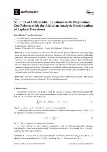
A structure preserving integrator may require additional computational cost and is not necessarily required for the complete system. Rewriting the reformulated system (1.5) as   F (t, x, x, ˙ z) 0 = F˜ (t, y, y) ˙ = (4.8) G(t, x, x, ˙ z, z) ˙ with G(t, x, x, ˙ z, z) ˙ = z(t) ˙ − gx (x, t)x˙ − gt (t, x), we can use different integrators for F and G and solve for (Xi+1 , Zi+1 ) either simultaneously, or iteratively with a dynamic iteration scheme [20], which is well understood for coupled ODEs. Example 4.4 (Example 4.2 continued) We use (4.8) and solve F with the implicit Euler and for G, we employ the two stage Lobatto IIIA method also known as (implicit) trapezoidal rule. This scheme preserves the invariant (4.7). Using the same settings as in Example 4.2 this approach yields an approximation with absolute error similar to the approximation of (4.4) with the implicit Euler method, as is illustrated in Figure 4.2.

Figure 4.2: Numerical solution (left) and absolute error (right) of (4.4), with the implicit Euler (blue, solid), and (4.5), with the combined Euler, LobattoIIIA approach (red, dashed).

5

Conclusion

The polynomial representation procedure introduced in [9] has been extended to a class of nonlinear differential-algebraic systems with well-defined strangeness index µ. It has been shown that the strangeness index is preserved during the polynomial representation. In particular, if the original system can be rewritten as an ODE, then the reformulated system is also an ODE. To avoid ill-conditioning, one should in general first derive the strangenessfree reformulation and then apply the polynomial representation procedure. The performed numerical study has shown that the time integration might require a different ODE solver to preserve additional invariants introduced by the polynomial reformulation.

References [1] A. Bellen and M. Zennaro. Numerical methods for delay differential equations. Clarendon Press, 2003. 17

[2] P. Benner and T. Breiten. Interpolation-base H2 -Model Reduction of bilinear control systems. SIAM J. Matrix Anal. Appl., 33(3):859–885, 2012. [3] A. G. Bratsos. The solution of the two-dimensional sine-gordon equation using the method of lines. J. Comput. Appl. Math., 206:251–277, 2007. [4] T. Breiten and T. Damm. Krylov subspace methods for model order reduction of bilinear control systems. Syst. Control Lett., 59(8):443–450, 2010. [5] S. L. Campbell. A general form for solvable linear time varying singular systems of differential equations. SIAM J. Math. Anal., 18:1101–1115, 1987. [6] S. L. Campbell and C. D. Meyer. Generalized Inverses of Linear Transformations. Pitman, San Francisco, CA, 1979. [7] T. Carleman. Application de la thorie des quations intgrales linaires aux systems d’quations diffrentielles non linaires. Acta Math., 59:63–87, 1932. [8] L. Dieci and T. Eirola. On smooth decompositions of matrices. SIAM J. Matrix Anal. Appl., 20(3):800–819, 1999. [9] C. Gu. QLMOR: a projection-based nonlinear model order reduction approach using quadratic-linear representation of nonlinear systems. Comput. Des. Integr. Circuits Syst., 30(9):1307–1320, 2011. [10] N. Guglielmi and E. Hairer. Computing breaking points in implicit delay differential equations. Adv. Comput. Math., 29(3):229–247, 2008. [11] P. Ha, V. Mehrmann, and A. Steinbrecher. Analysis of Linear Variable Coefficient Delay Differential-Algebraic Equations. J. Dyn. Differ. Equations, 26(3):1–26, 2014. [12] E. Hairer, C. Lubich, and G. Wanner. Geometric Numerical Integration: StructurePreserving Algorithms for Ordinary Differential Equations. Springer Series in Computational Mathematics. Springer-Verlag, 2006. [13] E. Hairer and G. Wanner. Solving Ordinary Differential Equations II: Stiff and Differential-Algebraic Problems. Springer-Verlag, Berlin, Germany, 2nd edition, 1996. [14] P. Kunkel and V. Mehrmann. Canonical forms for linear differential-algebraic equations with variable coefficients. J. Comput. Appl. Math., 56:225–259, 1994. [15] P. Kunkel and V. Mehrmann. Differential-Algebraic Equations. Analysis and Numerical Solution. European Mathematical Society, 2006. [16] P. Kunkel, V. Mehrmann, and I. Seufer. GENDA: A software package for the numerical solution of general nonlinear differential-algebraic equations. Preprint 730–2002, Institut f¨ ur Mathematik, TU Berlin, Str. des 17. Juni 136, D-10623 Berlin, FRG, 2002. [17] V. Mehrmann. Index concepts for differential-algebraic equations. Preprint 03–2012, Institut f¨ ur Mathematik, TU Berlin, Str. des 17. Juni 136, D-10623 Berlin, FRG, 2012. To appear in Encycl. Appl. Math.

18

[18] V. Mehrmann and C. Shi. Transformation of high order linear differential-algebraic systems to first order. Numer. Algorithms, 42:281–307, 2006. [19] V. Mehrmann and L. Wunderlich. Hybrid systems of differential-algebraic equations Analysis and numerical solution. J. Process Control, 19(8):1218–1228, 2009. [20] U. Miekkala and O. Nevanlinna. Convergence of dynamic iteration methods for initial value problems. SIAM J. Sci. Statist. Comput., 8(4):459–482, 1987. [21] M. P. Qu´er´e and G. Villard. An algorithm for the reduction of linear DAE. In A. H. M. Levelt, editor, Proceedings of the 1995 International Symposium on Symbolic and Algebraic Computation (ISSAC’95), pages 223–231. ACM Press, New York, NY, 1995. [22] W. J. Rugh. Nonlinear System Theory, The Volterra/Wiener Approach. The Johns Hopkins University Press, Baltimore and London, 1981.

19