closest, respectively, as it is also illustrated in Figure 1. ... Adobe® Photoshop® terminology, then consider colour .... Ï is the between-class variance. We.
INDEXING AND SEGMENTING COLOUR IMAGES USING NEIGHBOURHOOD SEQUENCES András Hajdu, Benedek Nagy, Zoltán Zörgö University of Debrecen, 4010, Debrecen PO Box 12, Hungary {hajdua|nbenedek|zorgoz}@math.klte.hu ABSTRACT In this paper we present some methods for indexing and segmenting colour images. The proposed procedures are based on well-known algorithms, but now we use digital distance functions generated by neighbourhood sequences to measure distance between colours. The application of such distance functions is quite natural and descriptive, since the colour coordinates of the pixels are non-negative integers. An additional interesting property of neighbourhood sequences that they do not generate metric in general, so we can obtain many distance functions in this way. We describe our methods for RGB images in details, but other image representations also could be considered. Moreover, the proposed methods can be applied in arbitrary dimensions without any difficulties.
1. INTRODUCTION Indexing and segmenting colour images is a very important field within digital image processing with growing interest. We can find a huge number of segmentation techniques [14] to solve a given problem in medical image processing, face detection, character recognition, etc. Many of these applications are based on some distance function to calculate the difference of the colours of the pixels. For historical reason, usually classic metrics are used, though a special distance function might be more suitable according to the nature of the problem. Since several colour image representations (RGB, CMYK, HSI, etc.) use integer colour coordinate values, thus digital distance functions also might be considered. This observation has led us to investigate the applicability of a family of digital distance functions. Since we obtained quite promising results, in this paper we would like to show how one can take advantage of using distance functions generated by neighbourhood sequences in colour image segmentation. The theory of neighbourhood sequences dates back to about 1968, when Rosenfeld and Pfaltz [15] recommended the alternate use of cityblock and chessboard motions for measuring distance in the two dimensional digital space Z2. In 1987, Das et al. [6]
extended the theory of periodic neighbourhood sequences to arbitrary dimension. The periodic property of such sequences were dropped by Fazekas et al. [9] in 2002. In Section 2, we give those concepts of this theory which we need in our further analysis. To illustrate our results, from Section 3 we consider the popular RGB model. However, we note that our methods also can be used in higher dimensions and other image representations, as well. The distance functions generated by neighbourhood sequences are not metrics in general. Nevertheless, in some cases non-metric distance functions also may provide nice results, thus it is not recommended to exclude them from analysis. Moreover, this way we have a lot more distance functions to choose from to refine our results. In Section 4, we show how colour image indexing and segmentation can be achieved by applying distance functions generated by neighbourhood sequences in simple distance measurement, region growing, and clustering. Our main goal is to call attention of the possible applicability of neighbourhood sequences in colour image segmentation. We do not focus on optimisation in our examples. Section 5 contains our practical experiments, and some recommendations to evaluate the obtained results. Finally, we make some conclusions in Section 6. 2. NEIGHBOURHOOD SEQUENCES In this section, we recall those concepts of the theory of neighbourhood sequences [9] which are essential in our investigations. Though we will consider the RGB image representation in details, we give the notions for arbitrary dimension, since our procedures can be applied to arbitrary dimensional integer image representations. From now on, let n be an arbitrary positive integer. Let q and r be two points in Zn. The i-th coordinate of the point q is indicated by Pri (q). Let m be an integer with 0 ≤ m ≤ n . The points q and r are m-neighbours, if the following two conditions hold: •
Pri (q) − Pri (r ) ≤ 1, 1 ≤ i ≤ n,
•
∑ Pri (q) − Pri (r ) ≤ m.
n
i =1
A sequence A = {a i }i∞=1 , where 1 ≤ ai ≤ n, i ∈ N, is called an nD-neighbourhood sequence. If a neighbourhood sequence is periodic, then for simplicity we write out only the members of a period to define the whole sequence. For example, we write {1,2} for the neighbourhood sequence {1,2,1,2,1,2,…}. We note that in practical applications with finite domain, it is usually sufficient to consider only the first "few" elements of a neighbourhood sequence. The point sequence q = q 0 , q1 , K , q j = r , where qi −1 and q i are ai -
neighbours for 1 ≤ i ≤ j − is called an A-path from q to r of length j. The A-distance d (q, r ; A) of q and r is defined as the length of the shortest path(s) between them. The distance function generated by the neighbourhood sequence A will be denoted by d(A). There exist a closed formula to calculate the A-distance for neighbourhood sequences [9]. Since in many segmentation and clustering techniques the Minkowski distances
and C3 (230,20,80). Now, if we calculate the distance of these colours with respect to the neighbourhood sequences {1}, {2}, and {3}, we get d (C1 , C 2 ;{1}) = 360, d (C1 , C 2 ;{2}) = 180, d (C1 , C 2 ;{3}) = 120,
d (C1 , C3 ;{1}) = 240, d (C1 , C3 ;{2}) = 180, d (C1 , C3 ;{3}) = 180, d (C2 , C3 ;{1}) = 300, d (C2 , C3 ;{2}) = 150, d (C2 , C3 ;{3}) = 150.
These values indicates that the distances of these colours highly depend on the neighbourhood sequence. More precisely, for the neighbourhood sequences {1}, {2}, and {3}, the colours (C1 , C3), (C2 , C3), and (C1 , C2) are the closest, respectively, as it is also illustrated in Figure 1.
1/ p
p⎞ ⎛ n L p ( q, r ) = ⎜ ∑ Pri ( q ) − Pri ( r ) ⎟ ⎠ ⎝ i =1
, p > 0,
n
L∞ (q, r ) = max Pri (q) − Pri (r ) i =1
are considered, we show the relationship between the Lp metrics and the distance functions generated by neighbourhood sequences, namely
Figure 1. The closest two among three colours, with respect to the neighbourhood sequences {1}, {2}, and {3}.
L1 (q, r ) = d (q, r;{1}) ≥ d (q, r; A) ≥ d (q, r;{n}) = L∞ (q, r ) holds for any nD-neighbourhood sequence A. As it is known from [6,9], not every neighbourhood sequence generates metric, and the existence of this property can be checked by a simple criterion [13]. However, if we do not need triangle inequality in our application, then we can use any neighbourhood sequences for measuring distance. Later we show examples with nice results obtained by such neighbourhood sequences that do not generate metrics. 3. MEASURING DISTANCE IN THE RGB CUBE BY NEIGHBOURHOOD SEQUENCES
4. APPLICATIONS
In this section we show how the theory of neighbourhood sequences can be used in classic colour image indexing and segmentation algorithms. We start with the generalisation of the "fuzziness" method referring to Adobe® Photoshop® terminology, then consider colour image segmentation with region growing, finally present an indexing method using cluster analysis. All of these methods are based on some distance functions which will be defined by neighbourhood sequences in the following examples. 4.1. Fuzziness
Colour image indexing and segmentation procedures are based on the comparison of the colour of the pixels. We use the 24-bit RGB cube (that is the domain is between black=(0,0,0) and white=(255,255,255)) to illustrate the descriptive behaviour of neighbourhood sequences in measuring the distance of two colours. By the following example, first we show that reasonable differences may occur according to the chosen neighbourhood sequence, thus it must be selected carefully to achieve the desired result. Let us consider the following three colours given by their RGB coordinates: C1(50,50,50), C2 (170,170,170),
This indexing procedure [10] selects those pixels which are within a given distance to one or more initially fixed seed colours. The implementation of this method also can be found in Adobe® Photoshop®, where it is referred to as the "Fuzziness" option [1]. To adjust the degree of fuzziness, one parameter (a distance threshold) can be given. As the first illustration of the applicability of neighbourhood sequences, we show some examples for the results of the fuzziness procedure, under using distance functions generated by different neighbourhood
sequences. Figures 2 and 3 below show the results of the fuzziness operation using one and more seed colours, respectively, and a threshold distance K for the maximum allowed distance from the seed colours.
Original image Original image
(a)
(b)
(a)
(b)
Figure 4. Region growing of stone parts using neighbourhood sequences with (a) one seed colour, (b) two seed colours.
4.3. Clustering
(c)
(d)
(e)
Figure 2. Fuzziness for seed colour with K=45, using neighbourhood sequences (a) {1}, (b) {211}, (c) {12}, (d) {2}, (e) {3}.
(a)
(b)
We recall an algorithm for indexing colour images based on cluster analysis [10]. In this procedure, the elements of the RGB cube are classified into clusters using a suitable metric. In our experiments, we used digital distance functions generated by neighbourhood sequences, and achieved promising results. To test our method, we chose hierarchical clustering [2] as a standard cluster analysis procedure with moving (and thus rounded) centroids to test our method. The clustering procedure starts with as many clusters as many colours are in the image, and merges those two clusters which are closest to each other at every step. In Figure 5 we show results for our clustering method with respect to different neighbourhood sequences.
(c)
Figure 3. Fuzziness for seed colours with K=25, using neighbourhood sequences (a) {1}, (b) {1112}, (c) {311}.
It is obvious that the result of the fuzziness operation highly depends on the chosen neighbourhood sequence. We mention that the neighbourhood sequences {211} in Figure 2(b), and {311} in Figure 3(c) do not generate metrics.
Original image
(a)
(b)
(c)
4.2. Region growing
To get a connected region, we can insert the distance functions used at fuzziness into a region growing algorithm (see [10,16]). After fixing seed colours, we start from a seed point (only spatial coordinates are important), and recursively grow the region with neighbouring points, whose colour values within a threshold distance K from the seed colours. Parameter K has a similar meaning than the "Tolerance" option of the "Magic Wand Tool" in Adobe® Photoshop® [1]. In Figure 4, we show some results for the proposed region growing algorithm.
Figure 5. Classifying colours into six clusters by neighbourhood sequences (a) {12}, (b) {23}, (c) {3}.
5. EXPERIMENTAL RESULTS AND EVALUATION
As we mentioned before, in this paper our main aim is to illustrate the capability of using neighbourhood sequences in colour image processing, and we did not focus on the
optimisation in our presented examples. In the followings, we summarise our experiences, and give some guidelines to help to find neighbourhood sequences which provides "optimal" results. 5.1. Fuzziness and region growing
Currently we are working on the implementation of the proposed methods for segmenting mineral types in images obtained by a microscope (see Figure 4). Our experiences show that the result of the segmentation can be improved reasonably by the careful selection of the seed colours, the neighbourhood sequence, and the distance threshold K. These parameters usually can be adjusted to the base mineral material type to obtain optimal result. For these kind of images we also suggest morphological postprocession to fill in the holes and gaps resulted e.g. by cracks. 5.2. Clustering
A quantitative analysis of our proposed clustering method can be obtained by considering suitable measures. For this purpose we calculated a specialisation of the uniformity measure proposed by Levine and Nazif [11], M
∑σ
E(I ) =
j =1
be worth taking into consideration in such procedures, since they are valid alternatives for integer domains. Especially, classic metrics are also can be approximated by distance functions generated by neighbourhood sequences; see e.g. [3,4,5,7,12] for the approximation of L2 in 2D and 3D. 7. REFERENCES [1] Adobe® Photoshop® User's Guide [2] M.R. Anderberg, Cluster Analysis for Application, Academic Press, NY, 1973. [3] M. Aswatha Kumar, J. Mukherjee, B.N. Chatterji, and P.P. Das, "A geometric approach to obtain best octagonal distances", Ninth Scandinavian Conf. Image Process., pp. 491-498, 1995. [4] P.E. Danielsson, "3D octagonal metrics", Scandinavian Conf. Image Process., pp. 727-736, 1993.
Eighth
[5] P.P. Das, "Best simple octagonal distances in digital geometry", J. Approx. Theory 68, pp. 155-174, 1992. [6] P.P. Das, P.P. Chakrabarti, and B.N. Chatterji, "Distance functions in digital geometry", Inform. Sci. 42, pp. 113-136, 1987. [7] P.P. Das, and B.N. Chatterji, "Octagonal distances for digital pictures", Inform. Sci. 50, pp. 123-150, 1990. [8] B. Everitt, Cluster Analysis, Heinemann Educational Books Ltd, London, 1973.
2 j
, Mσ 2 where M is the number of clusters, σ 2j is the j-th within-
[9] A. Fazekas, A. Hajdu, and L. Hajdu, "Lattice of generalized neighbourhood sequences in nD and ∞D, Publ. Math. Debrecen 60, pp. 405-427, 2002.
class variance, and σ 2 is the between-class variance. We note that E ( I ) ≥ 0 , and the less this value is, the better theoretical clustering result is assumed. In our method, E (I ) highly depends on the chosen neighbourhood sequence which is illustrated in Table 1.
[10] R.C. Gonzalez, and R.E. Woods, Digital image processing, Addison-Wesley, Reading, MA, 1992.
{1} {12} {13} 0,081 0,084 0,093
{31} {2} {23} {32} 0,076 0,064 0,057 0,084
{3} 0,091
Table 1. Quantitative analysis by E(I) of classifying colours in Figure 5 to six clusters using different neighbourhood sequences.
The above uniformity measure might be useful to find an optimal neighbourhood sequence. From the table it can be seen that it is also worth considering neighbourhood sequences (e.g. {31}, {32}) which do not generate metrics. 6. CONCLUSIONS In image indexing and segmentation techniques mostly the Euclidean (L2) metric is used, but other metrics (Lp, Mahalanobis, etc.) are also recommended, as they may provide better results in some cases (see e.g. [8]). In this paper we showed some examples to prove that distance functions based on neighbourhood sequences also might
[11] M.D. Levine, and A.M.Nazif, Dynamic measurement of computer generated image segmentations, IEEE trans. PAMI 7, pp. 155-164, 1985. [12] J. Mukherjee, P.P. Das, M. Aswatha Kumar, and B.N. Chatterji, "On approximating Euclidean metrics by digital distances in 2D and 3D", Pattern Recognition Lett. 21, pp. 573582, 2000. [13] B. Nagy, "Distance functions based on generalised neighbourhood sequences in finite and infinite dimensional spaces", 5th International Conference on Applied Informatics, Eger, Hungary, pp. 183-190, 2001. [14] N.R. Pal, and S.K. Pal, A Review on Image Segmentation Techniques, Pattern Recognition 26, pp. 1277-1294, 1993. [15] A. Rosenfeld, and J.L. Pfaltz, Distance functions on digital pictures, Pattern Recognition 1, pp. 33-61, 1968. [16] M. Sonka, V. Hlavac, and R. Boyle, Image processing, analysis, and machine vision, Brooks/Cole Publishing Company, Pacific Grove, CA, 1999.