Indexing XML Objects with Ordered Schema Trees Laurent Yeh, Georges Gardarin Laboratoire PRiSM Université de Versailles Saint-Quentin 78035 VERSAILLES CEDEX, France
[email protected] Abstract: XML DBMSs require new indexing techniques to efficiently process structural search and full-text search as integrated in XQuery. Much research has been done for indexing XML documents. In this paper we first survey some of them and suggest a classification scheme. It appears that most techniques are indexing on paths in XML documents and maintain a separated index on values. In some cases, the two indexes are merged and/or tags are encoded. We propose a new method called SIOUX that index XML values on ordered trees, i.e., two documents are in the same equivalence class is they have the same schema tree, with identical elements in order and number. The method can be seen as an extension of relational DBMS systems, where schemas are separated from data, and data are manipulated with their associated metadata. We use a simple benchmark to compare our method with two well-known European products. The results show that indexing on full trees is better for pure structural search in most cases.
1. Introduction 1.1
Problem
Since XML has been proposed as a standard exchange format by W3C, many database systems have been developed to store and retrieve XML documents. Most systems are supporting XPath queries and move towards supporting full XQuery, including XPath, FLWR expressions, and full-text search queries. Traditionally, database research distinguishes structure query from content query. Structure queries are dealing with hierarchical traversals of XML trees, i.e., processing the path expression in an XPath query. Content queries are searching for combinations of keywords and values in XML elements, i.e., processing the predicates in an XPath query. In modern XML servers, content search integrated with structure search must be efficiently performed.
1.2
Background
The support of structure and content queries require efficient indexing of XML documents. Much research has been carried out to propose and evaluate efficient indexing techniques. Traditionally, document-indexing systems were based on inverted lists giving for each significant keyword the document identifiers with the relative offsets of the keyword instances. With XML most queries are searching for elements rather than for full documents; thus, inverted lists are referencing element identifiers rather than simple document identifiers. However, numerous element identifiers may lead to large index difficult to manage. Structure query requires an efficient method to determine what nodes are parent or child of a given set of nodes. This can be done by performing structural joins on the edge (node, label, node) relation encoding the document structure [7], by traversing the document composition graph that is maintained when document are inserted [8, 16, 3], or by using clever numbering schemes for node identifiers [5, 15, 14]. Another problem with structure queries is that regular expressions are used extensively. Thus, label paths may be partial, including simple (*) or recursive (//) wildcards. This may lead to recursive structural joins or navigation in entire XML data graphs. Notice that structural joins and numbering schemes may also be used to check ancestor and descendant relationships, thus helping in solving regular expressions. To overcome these difficulties, structural summaries of XML document collections have been proposed. Dataguides extended with node references were first introduced in Lore [13]. The structural index is in
1
general quite large as every database node is referenced within the index. Several path index structures as Tindexes [16] and APEX [2] tried to reduce the index size by indexing only useful paths. Such paths can be determined by specific patterns (T-indexes) or by selecting the most frequently used paths in queries (APEX). The Fabric index [3] avoids referencing all nodes by encoding paths of terminal nodes (leaves) and storing them in a balanced Patricia trie. However, this approach requires extensions to maintain path order and to perform partial matching of tags. Numbering schemes have been implemented in Xyleme, a successful native XML DBMS [1]. Two schemes are possible: pre and post-order numbering of nodes (a node identifier is a triple pre-traversal order, posttraversal-order, level) and hierarchical addressing of nodes (a node identifier is the compaction of its rank at each level). In both cases, determining if a node is an ancestor or a parent of another is simply done by comparing the identifiers. Xyleme manages a value and structure mixed index giving the node identifier of each label and of each keyword. In addition, for each XML collection, Xyleme maintains a generalized DTD, i.e., the set of paths with cardinalities. Solving an Xpath expression is mostly done through index accesses, i.e., determining for each label and keywords in the Xpath the relevant nodes identifiers and intersecting them. The method is quite efficient, but as with the others, the index references all database nodes. It is managed in main memory, which makes that some applications require large main memory.
1.3
Paper Contributions
In this paper, we first review the main methods proposed to index XML data. They all maintain a path-based structural summary with references to database nodes. In general, two nodes are in the same equivalence class if they have the same incoming path set. We describe a new method named SIOUX implemented in the Reposix prototype at University of Versailles, which maintains enriched structural summaries without full references to database nodes. The structural summary of a document is graph-based, i.e., it keeps element order and multiplicity of elements. Two documents are in the same equivalence class is they have the same schema tree, with identical elements in order and number. The structural index only keeps document references, not node references. The graph-based structural summary is rich enough to make possible computing the node identifiers for qualifying path expressions. The method is centered around a structural index comprising a repository of schemas memorized as XML tree structures (XML documents without leave contents). An XML tree structure is called a schema tree. The repository delivers a schema identifier for a given schema tree. The repository of schema trees is at the heart of the structure index, which keeps for each schema tree the list of document identifiers having this exact schema. The fundamental idea of the method is to index documents by sequences of paths rather than by paths. It results from the observation that path order is generally meaningful (for example, most articles starts with a title and finishes with a conclusion, not the reverse). Keeping precise structural guides avoid memorizing node identifiers as they can be computed from the schema tree for a query path expression. The method is very effective with documents of irregular schemas. In addition, the method integrates a value index, which gives for each keyword occurring in a terminal node the node identifier and the relative position in node content. Several forms of node identifiers can be used, e.g., the hierarchical address or preorder number. The value index could be replaced by a signature file, a well-known technique in information retrieval [6]. The advantage of a signature file is to be more compact than a value index, but the disadvantage is to be less precise and retrieve noise that has to be eliminated by value checking before returning the qualifying elements. We also propose to extend the document structure with a content signature as an additional tag to make schema trees a more differencing structure in case of too many documents of similar structure. To solve an Xpath expression of the form /Book/Author[contains(Address, "Paris")], the system: (i) search for all path trees containing the path /Book/Author/Address, then determines their possible documents and node identifiers through the structural index; (ii) search for all nodes containing "Paris" through the value index; (iii) do the intersection of the two lists of node identifiers to finally return the list of qualifying nodes. It is efficient in general and can be extended with OR and NOT predicates. In addition, if certain lists become too large before intersecting them, they can be ignored and replaced by checking all the documents of the other list. This is the case when all documents have exactly the same tree structure for the structure part of the query, or when all elements contain the searched keywords for the value part of the query.
2
Finally, we present an evaluation of our method. An hybrid benchmark with documents of varying schemas run on three systems demonstrates both the compactness and the efficiency of our structure indexing scheme.
1.4
Outline
In this paper, we compare existing indexing schemes for XML data and propose a new hybrid method that looks rather promising. First, we review some of the research proposals for indexing XML collections. We give a summary of each selected technique and then informally review it at the light of simple evaluation criteria. We also introduce the indexing schemes of two XML database systems: Xyleme and X-Hive. Next, we introduce a new method called SIOUX implemented in a research prototype. Finally, we propose a simple benchmark for evaluating indexing methods. It is run on the three systems and gives rather promising results for the SIOUX method, at least for structure queries.
2. Overview of Existing Indexing Schemes In this section, we first discuss the main issues to design an indexing scheme. Next, we review some of the most well known schemes and give informal evaluations for each of them.
2.1
Evaluation criteria
As pointed out above, many approaches to XML indexing have been proposed. What are the relevant criteria to consider when selecting one index type? In the sequel, we introduce a few that we believe important and that we shall use to compare proposed methods. Type of identifiers All methods require document identifiers and most uses also node identifiers within documents. Node identifiers can be composed of one or more numbers in complement to a document identifier. They can be attributed in such a way that they memorize the parent-child relationships. The disadvantage of not having element identifiers in the index is that post-processing is required to locate document elements after selecting documents through the index. If the number of selected documents is large and if documents are also large, post-processing might be considerable [15]. However, if document are small with complex structures, node identifiers may become costly in place. Structural Search Most XPath queries involve the exploration of the descendant (and sometimes the ancestor) of a given set of nodes. A naïve approach is to use join algorithms on the parent-child relation, which is time consuming in general. However, join algorithms can be improved using for example B-tree structures. Another solution is to maintain and navigate the graph structure of the documents. The most sophisticated algorithms are based on element numbering schemes that determine if a node is an ancestor or a descendant of another simply by comparing identifiers. Keyword Search Keyword search and its many variations must be efficiently performed, notably to support the CONTAINS predicate of XQuery and the new developments in XQuery Text. In general, keyword search requires a specific index, in its simplest form an inverted list implemented as a B+-tree. Signatures, i.e., Boolean vectors resulting from hashing keywords present in documents or elements, have also been used in traditional information retrieval systems. Inverted lists have been sometimes mixed with structural indexes. To efficiently support XQuery text, the capabilities of prefix, postfix, infix search are important. So is the capability of measuring the distance of two words (in words) in a document. Further, similarity search may require evaluation of semantic proximity of elements. This is achieved in document systems through vector encoding of documents using classical tf-idf (term frequency - inverse document frequency) weight of the important words in a document. Few indexes are supporting similarity search. Size of indexes The size of the index is an important criterion. The size of an index depends on the number of entries (e.g., one per document, one per each element, or one per terminal element) but also of the average size of an entry. In general, there is one entry per important word in document content; in addition, certain index requires one entry per name of elements. Graph index may list all paths in documents. For each entry,
3
relevant documents are referenced, with optionally a list of relevant node identifiers per document. Keeping the index small is a good heuristics. Document Update The behaviour of an index when documents are updated is an important issue. Some types of index are not robust when documents are updated and must be rebuilt, at least for the updated document. Others are incremental and only require deletion and addition of updated elements. In between, solutions have been proposed that are robust for a limited amount of updates per document. Query Benchmark Comparing performance of index schemes is always difficult. In general, each proposal presents some experimental results that compare with one or two other approaches by varying some parameters. Traditionally, the collection of the plays of Shakespeare, the XMark benchmark [20]and benchmark generated from DTDs using the XML Generator from IBM are used. While Shakespeare and XMark are trees, some graph structured XML can be generated using the Flix Markup Language (FlixML) for movie reviews and the GedML markup language for the genealogical XML data. Most benchmarks specifies regular DTDs for XML documents. We are interested in irregular document structures, where few documents share the same DTD. Comparing index size is easy but comparing query performance is a more difficult issue. With XQuery, a large panoply of queries can be expressed, including free-text searches [22]. A significant benchmark has to cover most cases without being too complex, which is a difficult compromise.
2.2
Indexing Rooted Paths: The Targeted Dataguide
Dataguides have been proposed by Goldman & Widom at VLDB97 [8]. They can be perceived as dynamic schemas, but are often extended with targeted node identifiers to serve as index. Such indexes are called targeted dataguide. Dataguide can also helps in query formulation. They are rather concise and accurate structural summaries. Every path in the database has one and only one corresponding path in the dataguide with the same sequence of labels. A rooted label path of a node is a sequence of labels defining a path from the root to the node. To achieve conciseness, a DataGuide describes every unique rooted label path of a collection exactly once. To ensure accuracy a DataGuide encodes no rooted label path that does not appear in the collection. In Laure [13], a dataguide is itself represented as an XML object, but this is an implementation option. Dataguides for a given collection of documents are in general not unique. A strong dataguide is such that any indistinguishable rooted label paths p and p' on the dataguide are also indistinguishable on the database (i.e., p(G)=p'(G) => p(DB) = p'(DB)). A strong dataguide is unique for a given collection of XML documents. Targeted dataguides store for each path node identifiers corresponding to elements having the given path labels. The index is thus an unordered graph with a list of document and node identifier for each path of length 1 to N. Dataguides are difficult to maintain for documents with cycle as paths should be limited in size. For searching on keywords, nothing is provided and an additional value index shall be maintained as in Lore [8]. The main properties of the Targeted Dataguide index are summarized in table 1.
2.3
Indexing Template-compliant Paths: The T-index
A template-based indexing technique (T-index) has been proposed by [16]. The idea is to build indexes not on all paths, but on selected path templates. The technique consists in grouping database objects into equivalence classes containing objects that are indistinguishable w.r.t to a class of paths defined by a path template. A path template t has the form T1 T2 … Tn where each Ti is either a regular path expression or one of the following two placeholders P and F. A query path q is obtained from t by instantiating each of the P placeholders by some regular path expressions and each of the F placeholders by some formula. T-index indexes all sequences of objects connected by a sequence of path expressions in conformance with the template. T-indexes are very general, as the template generator cover a wide range of paths, including all paths, paths with given prefix, postfix, etc. There are interesting particular cases. 1-index indexes all objects reachable through an arbitrary path expression P from a root. 1-index is a non-deterministic version of the strong data guide and coincide with it for tree-structured data. 2-index indexes all pairs of objects connected by an arbitrary path expression P. While each T-index is designed for a particular class of queries given by one
4
template, it can be used to answer queries of more general forms. Computing this equivalence relation may be expensive (PSPACE complete), so the authors consider finer equivalence classes defined by bisimulation or simulation, which are efficiently computable. A T-index is built from these equivalence classes by constructing a non-deterministic automaton whose states represent the equivalence classes and whose transitions correspond to edges between objects in those classes. The beauty of T-indexes is the generality and the fact that T-index can be used to help solving a wide variety of queries. A T-index behaves like a concrete view of the database that can be used to reformulate queries and solve them more efficiently. T-index main properties are summarized in table 1.
2.4
Indexing Frequently Used Paths: APEX
APEX is a method to manage adaptative path indexes for XML data [2]. While the strong dataguide maintains all paths from the root, APEX does not keep all but utilizes frequently used paths to improve query performance. APEX maintains in the index all paths of length 1 plus additional required paths, i.e., the set of labels plus some composed paths, those that are frequently queried. APEX assumes the existence of a database maintaining the query workload and determines frequently queried paths by selecting those above a given support. An APEX index consists of two structures, a graph structure representing the structural summary of the data, and a hash tree structure that associates required paths to nodes of the graph structure. For efficiency, each node of the hash tree is implemented as a hash table on the labels. Terminal nodes refer to a graph structure node. The hash tree is used to find nodes of the structure graph for given label path, also for incremental update. A graph structure node contains the list of node identifiers of the XML documents, similarly to a targeted dataguide node. The APEX graph structure is simpler that the dataguide and accessed through the hash tree. Nice algorithms are proposed to perform incremental updates of the hash tree and graph structure. APEX main properties are summarized in table 1.
2.5
Indexing Rooted Paths with Values: The Index Fabric
The index Fabric has been introduced by [3]. It includes both an efficient implementation of the dataguide and a clever extension with values in place of identifiers. To shorten the paths, labels are first encoded with one or more (if required) letter. All paths from the root to a leave containing data are prearranged as a sequence of encoded labels followed by the value as a string. For example, the path /Restaurant/Adress/City[Paris] is encoded as RACParis. To store the encoded strings, the method uses an efficient index for strings, i.e., a Patricia trie. A Patricia trie is a simple form of compressed trie that merges single child nodes with their parents. A balancing mechanism is added to the Pratricia tree to guarantee constant access time when searching for paths of length N. Path expressions including predicates on values for elements are performed as string search. Notice that the index does not keep information on non-terminal nodes. It does not manage node identifiers either. Also, it does not keep the order of elements in documents although it stores terminal node values. Table 1 gives an overview of the main properties of the index Fabric.
2.6
Indexing Values and Labels with Structural Node Identifiers
Several methods have been proposed to replace the structural graph index by a node numbering scheme. Node identifiers (NID) determine elements in documents themselves identified by a document identifier (DID). The NID attribution device aims at replacing structural joins by function computations: is_parent(NID1,NID2) and is_ancestor(NID1,NID2) are simple and efficient functions to check the parent and ancestor relationships. We detail some of the proposed schemes below. Some schemes have been proposed to make identifiers stable in presence of updates. Virtual Node Identifiers A simple scheme has been proposed in [15]. The document structure is mapped on a k-ary tree (see Figure 1). Node identifiers are assigned according to the level-order tree traversal. The parent of node i is parent(i) = (i-2)/k + 1 and the j-th child of node i is child(i,j) = k(i-1) + j + 1, k being the arity of the virtual tree. Among the virtual children of node i, be {k(i-1)+j+1 | j=1, k}, only ri ≤ k are real nodes. The determination of the real existence of a node can be done in several way, e.g., using a bitmap associated to each document.
5
Figure 1: Mapping a document to a virtual tree [15]
Although the method is simple and effective, the determination of the real existence of parent/child relationships and the choice of the arity of the tree are difficulties. Updates require reassigning all node identifiers when documents become larger in some nodes that the arity of the virtual tree. Selecting a large arity implies large identifiers and bitmaps. The authors suggest the possibility to have different arities per level, which is complex. Pre-Post Order and Tree Level Identifiers in Xyleme Xyleme is an efficient XML warehouse used in several document-oriented applications. One key feature of Xyleme is its indexing mechanism, which makes possible to process most text-oriented queries without accessing the data. Xyleme stores XML DOM trees in pages using the NATIX (from Mannheim University) repository, which compresses and maps XML trees on one or more pages. Xyleme keeps document ID and element ID. While document IDs are simple references, two forms of element ID are supported: • •
The bit-structured scheme gives the structural position of the node by level in the tree. For example, the node e in Figure 1, will be identified by 1.1.2. Thus, a NID clearly lists all ancestors of the context node. The prefix-postfix scheme proposed in [5] keep the preorder and postorder of each node as identifier, generated by a left-deep traversal of the document tree. For example, the node e in Figure 1, will be identified by (7,4). The ancestor relationship is determined by X ancestor of Y iff pre(X) < pre(Y) and post(X) > post(Y).
Using these types of identifiers, Xyleme maintains an index of labels and values (keywords of contents). To solve an XPath query, the index is accessed with given labels and word predicates, then lists of identifiers are processed to check ancestor/descendant relationships and conjunction/disjunction of conditions. The index is kept in memory and the selected elements can be accessed in parallel by the repositories implemented on multiple computers. Table 1 sums up the main indexing features of Xyleme. Interval Encoding A storage efficient technique to identify XML nodes and keep document size is known as interval encoding. It has been used to store efficiently XML documents in relational databases. The general format consists in associating a pair of values (order, size) to each node in the XML graph, such that x is ancestor of y iff order(x) < order(y) ≤order(x) + size(x) [4]. One way to generate a valid interval encoding is to perform a depth-first traversal of the document tree, using an incrementing counter that assigns the left value to a node when it is first encountered, and the right value when the node is seen for the last time. This is simply a refinement of the Dietz numbering scheme. It can be made resilient for updates by keeping size for them. Node identifiers generated by interval encoding are also useful to keep offset of keywords in value index. Relative Region Coordinates To deal with the content update problem that is not adequately addressed in most numbering proposals, [11] features a specific mechanism called relative region coordinates. The idea is to express the coordinate of an XML element in relation to its parent element coordinates: the start and the end of a node are relative to the parent start. Using the relative region coordinate to locate XML elements, we know only where the elements start and end inside the region of their parent elements.
6
As in index related coordinates are stored together, we need to update only a portion of index file in case of content updating. Also, it is possible to compute the absolute region coordinate of an element by summing up the relative region coordinates of its ancestors and itself. In consequence, the indexing scheme requires update of only a small portion of index file in case of updating.
2.7
Overview and Classification of Indexing Techniques
Table 1 gives an overview of the main features of the main analyzed indexing techniques. We add XHive [21] as it is an interesting product that we use for benchmarking. Identifiers are in general document identifiers plus node identifiers. Node identifiers can be composed of prefix/postfix or hierarchical addresses as in Xyleme. This avoids structural join and navigation. The index Fabric does not use node identifiers. The size of indexes is generally linear in function of the number of nodes and the number of paths. Two methods are clearly targeted towards solving regular path expressions with wildcards.
Data Guide
T-Index
APEX
FABRIC
XYLEME
DID+NID 2 Int Navigation
DID+NID 2 Int Navigation Direct
DID+NID 2 Int Navigation Direct
DID 1 Int Encoding+ Trie search
DID+NID DID+NID 2 Int+Int|bits 3 Int Check inegalities Join on element Index
Value index
Value index
Value index
Trie search + Scan
Index search
Value Index
Global
Global
Incremental
Incremental
Incremental
Index Size
NumPath+ NumNode
SelePath+ NumNode
NumLabel+ NumPath
NumPath
Partial match
Possible
Possible
NumLabel+ SelectedPath+ NumNode Targeted
Targeted
Possible
Live increment. Non-Live global NumLabel+ SelectedPath+ NumNode+ … Possible
Identifiers Structure Search Keyword Search Update
X-HIVE
Table 1: Overview and synthesis of some indexing methods
The reviewed indexing techniques can be presented in a classification hierarchy as portrayed in Figure 2. The first level classifies methods according to the technique used for resolving hierarchical path expressions. Methods using graph traversal maintains some form of dataguide, i.e., an index of all rooted paths. Fabric used an encoding of all paths stored in a Patricia trie that can be explored using text search. Methods based on a numbering scheme requires an additional index containing at least one entry per label (often merged with the value index); this index is the starting point of the search to get lists of identifiers that can be compared. Notice that the reviewed indexing techniques use label and often paths as index entries, which makes index large in general. All index forget about path orders and number of occurrences. Furthermore, most methods except Fabric have difficulties with intensive updates, either to maintain index entries or identifiers. XML Indexing Methods
T-Index
Hierarchy
Fabric Dataguide
Numbering Scheme
Text Search
Graph Traversal
APEX
Pre/Post Order
RRC
Interval Encoding
Figure 2: Classification of some XML indexing methods
7
3. A New Indexing Scheme Based on Schema Tree We propose a new index scheme coupling a structure index and a value index. The structure index is based on (optionally signed) schema tree, a finer data structure than dataguide: index entries are ordered trees rather than paths. The value index is a conventional inverted list. Signatures files could also be considered and are a bit discussed.
3.1
The Structural Index
The structural index defines equivalent classes of documents, one class for each XML structure existing in the database. The structure is called a schema tree. Definition 1: Schema Tree. Let x be an XML document. A schema tree ST(x) is an ordered tree that includes exactly k instances of every label paths present k times in x and keeps the same order of elements for the corresponding nodes of x and ST(x). Notice that a schema tree differs from a dataguide as multiple paths and elements in different orders are distinguished; also, it is not an index but a document structure, with no reference to data. For simplicity, we consider only trees although the definition could be extended to graphs with cycles (for encoding references). Attributes in documents are processed as elements, but the order of attributes is irrelevant. To deal with attributes as elements, we include them as the first children of the node they are attached to and we order them by alphabetical order. Definition 2: Schema Tree Index. Let C be a collection of XML documents x1, x2, …xn. A schema tree index gives for each different schema tree of the document collection the list of documents xi having this schema tree. A schema tree index shall implement efficiently the following functions: • • • • •
Retrieve a given schema tree if it exists. Retrieve all documents of a given schema tree. Add a given document xn+1 in the collection and maintain the index. Delete a given document xi from the collection and maintain the index. Find all documents satisfying a given XPath in the collection.
We discuss in the next section possible implementations of schema tree index and describe our. It is important to notice that a schema tree index defines equivalent classes of documents per schema, i.e., xi ≡ xj iff the ST(xi) = ST(xj). Unlike current indexing schemes, we maintain an index with one entry per schema tree and not per path. Also, the schema tree index references objects and not elements. However, as schema trees distinguish orders and duplicates, the index is able to deliver the hierarchical address (i.e., 1.2.5 for node 1, child 2, child 5) of any node satisfying a path. Schema trees are richer than dataguides and avoid storing node identifiers within the structural index, which saves in index size (see evaluation). In the case of a homogeneous collection of objects having an identical schema tree, our structure index will have only one entry giving the list of objects. To avoid such situation, if an entry of the index is too large, we propose to add signatures of objects to further distinguish the equivalent objects; thus, xi ≡ xj iff SST(xi) = SST(xj), where SST stands for Signed Schema Tree. Let us recall that a signature of an element is the binary encoding of some hash function on [0,N] applied to each keywords of the element. Thus, a signed schema tree can be seen as a schema tree plus an empty tag whose label is the signature. Definition 3: Signed Schema Tree Index. Let C be a collection of XML documents x1, x2, …xn. A signed schema tree index gives for each different signed schema tree of the document collection the list of documents xi having this signed schema tree. The generation of the signature tag can be seen as a pre-processing step adding a signature labelled tag to the document. It can also be integrated dynamically to the signed schema tree index functions: signatures can be generated to split dynamically index entries that are too large. Notice also that signature can be used to focus on path queries with keywords predicates (i.e., CONTAINS(., “keywords”)): only entries with relevant signatures for the given keywords have to be retrieved. We will not develop further this possibility to distinguish schema with signatures, but this can be useful in case of many documents of similar structure to develop some extensible partitioning through schemas.
8
3.2
The Value Index
To accelerate value search (exact match, less or greater predicates, keywords, phrase match, etc.), we use a classical inverted list scheme. For each keyword appearing as element or attribute value, the value index gives the document id, the identifier of the element in a given ST, and the offset of the keyword in the element. The value index could be organized as a B-tree or a hash table; we implement the last solution. Definition 4: Value Index. The value index is a mapping giving for each keyword the list of document identifiers with the node identifiers and relative addresses of elements containing the keyword. An alternative possible organization for the value search accelerator consists in using a signature file. The storage utilization of signature file is better than that of the inverted list. Each content enclosing element or attribute (i.e., leaf node) of an XML file can be signed. A signature file can be represented as table SIGN (DocId, EleId, signature), where DocId is a document identifier, EleId an element identifier, and signature is computed by setting to 1 only the bits whose ranks result from the hash function applied to an element keyword. Giving a list of keywords, the hash function determines a signature s. All couples whose associated signatures include s are potential candidates for answering the value search. While the value index determines exactly the matching elements, the signature file determines only possible matching elements. One or the other structure can be used in conjunction with our structure index, which is a nice feature. For simplicity, we implement the value index as explained below.
4. Maintaining Schema Tree Index As explained above, the schema tree index keeps the mapping between schema trees and documents. The structure has to be efficient, compact, and extensible (e.g., to support signature). We divide the mapping in two steps: (i) mapping Schema Trees (ST) to schema tree identifiers; (ii) mapping schema tree identifiers (STI) to XML objects.
4.1
Mapping schema trees to schema tree identifiers
All schema trees are integrated in a union tree as exemplified in Figure 3. This global schema tree structure (GST) is optimized. It is a graph in which: (i) A node represent an XML element or attribute of one or more schema trees. (ii) An edge represents either a parent / child (down edge) or a preceding / following sibling relationship (next edge) in at least one XML tree. To reduce the size of the union graph, the lists of nodes at a given level in the union tree are merged together in sequence order in such a way that the total list be minimum in number of entries. Thus, all nodes at a given level are linked together, but schema trees are distinguished by identifiers as explained below. Nodes are labelled with the corresponding element name or attribute name prefixed by @. To be able to retrieve a schema tree, nodes belonging to a schema tree are marked with the corresponding schema tree identifier. In other words, the set of schema tree identifiers a node belongs to is added to its label (e.g., book: 1,2). The order of element nodes in each schema tree is preserved at each level. The GST can be updated by inserting nodes at existing levels or at a new bottom level. Root Book:1,2
Level 1 Person:2,3
Author:1,2
Editor:2
Name:1
Address:1
Book:3
Level 2 Level 3 Level 4
@Title:1 Figure 3: Example of GST
To extract a ST of given identifier STI from the GST, a simple procedure consists in traversing the tree and extracting all nodes of identifier STI with the corresponding edges. The advantage of the proposed structure is to make possible the factorisation of nodes at the same level in all ST. If a node exists for a given ST at a given level, the cost to represent it for another ST is an identifier (an integer indeed). The GST is thus a
9
structure whose number of nodes in worst case is the number of element and attribute pathnames in the database. Thus this is similar to a structural guide. Notice that if an STI appears in a node, all its ancestors shall contain this STI as a ST containing a path contains also all its sub-paths.
4.2
Mapping schema tree identifiers to XML objects
We use a simple indexed table MAP_STI to map a schema tree identifier to an XML object. The entry number in the table corresponds to the STI. STI are integers allocated from 1 to N; when a ST is deleted, the STI is marked free for latter allocation to a new schema tree. The table is composed of two columns as shown in Figure 4. The first contains the number of objects with the given schema tree, the second is a pointer to the first bucket containing the XML object identifiers. The table is maintained in main memory. A swapping mechanism is implemented to write it on disk when required. Identifier buckets are of fixed size and simply organized in a chained list.
In main memory Card
Pt
1
3
1244
2
3
343
1
3454
3
Id1,id2,…
Id8,...
Id3,id6,id11
Id3,id6,id11 ...
...
...
Figure 4: The mapping of schema tree identifiers to matching objects
4.3
Indexing values
Each value of an atomic type (e.g., numeric, date, url) or significant keyword for text type is indexed through an inverted list. Significant keywords in texts are simply determined from a list of excluded words (e.g., stop words). The inverted list is organized as a hash table mapping each constant value to a list of doublet . The node identifier is a number identifying the node in the schema tree (we use a pre-order traversal to identify nodes but other numbering schemas are possible). The offset of the word could be additionally memorized for answering queries of type "word followed by word" or "phrase search", as required in XQuery Text. An interesting alternative would be to use an extensible hashed file on keys to store and retrieve . The advantage would be to access directly to elements of searched path for a given keyword. This would be efficient to solve queries such as /Book/Author[contains(Address, "Paris")]: the GST and its associated MAP_STI will determine objects with structure /Book/Author/Address and compute the Address node identifier; the hashing will determine objects with value "Paris" for the relevant node identifier. Let us point out that node identifiers are simple integers obtained by traversing the tree in some fixed order (e.g., pre-order). From the GST, the ST of an object of given identifier can be extracted as explained above. Thus, a parallel traversal of the ST and the object is possible to determine the node content. The fundamental of our method is to manipulate an object always in association with its schema (a tree), as well as in traditional relational DBMSs (a table structure). Thus, node identifiers can be derived from schema trees and encoded as compact integers.
4.4
Searching a Schema Tree
When inserting a new XML object in the database, it is required to determine if the associated schema tree already exists in the GST. If it exists, the schema tree identifier is simply returned; the constant values of the leaves are indexed and the object can be inserted. If it does not exist, the new schema tree must be inserted in the GST with a new STI, and the document reference is inserted in the MAP_STI table
10
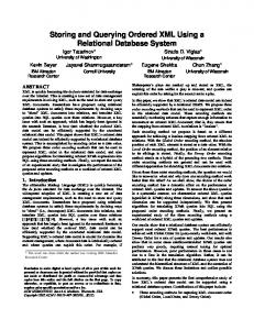
The search problem of an ST in a GST can be seen as an extension of the well know "tree pattern matching" problem [18, 10]. The general problem can be formulated as follows: given two labeled ordered trees, the pattern and the target, find all occurrences of the pattern in the target. In our case, the pattern is ST and the target GST. In addition, several constraints have to be fulfilled: (i) Nodes are marked with identifiers so that we only accept patterns whose nodes are all marked with a common identifier. (ii) The matching nodes have to be of same depth. (iii) The pattern has to be strictly included, without additional leaves. In the problem of ordered tree inclusion two ordered labeled trees P and T are given, and the pattern tree P matches the target tree T at a node x, if there exists a one-to-one map f from the nodes of P to the nodes of T which preserves the labels, the ancestor relation and the left-to-right ordering of the nodes. More precisely, the problem can be formalized as follows: we have to find a one-to-one map fi from the nodes of ST to the nodes of GST which preserves:
1. The root: The root of ST maps to the root of GST. 2. The labels with a common identifier i: ∀ v ∈ ST, v and fi(v) have the same label with identifier i among their set of identifiers. 3. The left-to-right ordering of the nodes: ∀ v1, v2 ∈ ST, v1 is left of v2 ⇔ fi(v1) is left of fi(v2) 4. The depth of the trees: ∀ v1, v2 ∈ ST, v1 is at the same depth that v2 ⇔ fi(v1) is at the same depth that fi(v2) -1 5. The covering of all nodes in GSTi: ∀ v ∈ GSTi, fi (v) ∈ ST. The algorithm to check the existence of a schema tree in the GST is given in annex. We adapt the tree pattern matching algorithm of [18] to our problem by supporting the additional constraints. The algorithmic cost is in O(s+g) where s is the number of nodes of ST, g is the number of nodes of GST. This cost is clearly less than this of well known "tree pattern matching" algorithms (e.g., cost is of order s*g in [10]). This is due to the fact that we are in a particular case with the supplementary constraints described above. The method is illustrated in Figure 5. It portrays a simple GST and three schema trees denoted ST1, ST2 and ST3. Let us exemplify the algorithm with ST1. The algorithm starts at the root and tries to match the trees level by level. At level 1, GST.A matches with ST1.A; thus, candidates schema trees are GoodST= {1,3,4}. GST.D does not match with B:2,3; thus, schema trees {2,3} cannot be candidates (BadST={2,3}). GST.D matches with ST1.D, thus GoodST={1,3,4} ∩ {4} = {4} is the only remaining candidate, which is selected as not in BadST. ST2 is not included in GST as there is no C node at level 1 in GST. ST3 is not included too as B is present (thus GoodST={2,3}) but A is not present, neither D, neither the second occurrence of A; thus BadST={1,2,3,4}, which yields that 2 and 3 are excluded.
Root
Root
GST
A:1,3,4
B:2,3
B:1,3
…
D:4
E:2
Root
ST1
A D Included (4)
A
A:2
Root
ST2 B
ST3
B
C
Not included ()
…
Not included ()
Figure 5: Searching an ST in a GST
11
4.5
Inserting a New Schema Tree
We now present the insertion of a new schema tree ST in a global schema tree GST. The global schema tree does not contain ST. The insertion proceeds recursively level by level. The problem is to find the best matching sub-sequence for each level, so as to limit the size of the GST. The insertion algorithm is given in annex. We describe the principles with a simple example below. Let S be a sequence of tags to insert at level i. For example, consider the insertion of ST2 in GST of Figure 5; at level 1, S= (AÆBÆC). For each tag in S, the algorithm searches for all positions where it appears if any. For example, A appears in 1 and 4; B in 2; C nowhere. Next, all possible placements for matching letters are checked. The best placement is the one with maximum matches; in case of several with same score, the first is simply selected. For example, A can be placed in 1 and B in 2, C being anywhere after 2, say 3; the score of this placement is 2. A can also be placed in 4, B in 5, and C in 6; the score of this placement is 1; thus the first placement with A in 1, B in 2 and C in 3 is selected. Finally, all tags in the selected placement have to be marked with the new ST identifier.
4.6
Deleting a Schema Tree
A schema tree is deleted when no XML document conforms anymore to its structure. The deletion is triggered when the count of objects with the given schema tree becomes 0 (Card= 0 in MAP_STI table, see Figure 4). To remove the ST in GST, we remove the STI from any node containing it. If a node contains no more STI, the node is removed. This requires a traversal of the GST tree.
4.7
Resolving XPath Expression
In this section, we introduce the XPath query processing algorithm using the schema tree index and the value index. For simplicity, we consider queries of the form (they can be easily written in XQuery):
SELECT XPath2* WHERE XPath1* formally written { XPath2*| XPath1* }. XPath1 are filtering expressions and XPath2 are projection expressions. XPath can be as general as defined in W3C XPath version 1.0. For simplicity, we consider only conjunctive queries but disjunctions could be supported easily in WHERE clauses. The process can be divided in three steps: (i) Determine the STI that verifies the structural constraints. (ii) Compute the relevant element references. (iii) Extract the response elements in main memory. Determination of relevant schema tree This step consists in extracting from all regular path expressions in the query the label paths that are mandatory for the query. From the set of label paths, a simple search in the GST of all STs including these label paths returns the relevant schema tree identifiers. For example, let us consider the query: SELECT /Book/Author/@speciality WHERE /Book/Author[contains(.,"John") and Address/City= "Paris" ]//Company}.
The required label paths are: { /Book/Author/@speciality | /Book/Author, /Book/Author/Address/City, /Book/Author//Company}.
The algorithm for determining the relevant STIs simply search each path expression in the GST. For each, it collects all the instances and returns the list of all STIs corresponding to the end-path nodes. Wildcards (*, //) have to be included in the search allowing to search for children or descendants of given name. Expanded path expressions in which wildcards are replaced by effective label paths are inserted in the set of required label paths in place of path expressions with wildcard, so as to memorize effective paths. To search a label path in the GST, we use an extension of the tree pattern matching algorithm [10]. The precise algorithm is described in annex. It is different from the ST searching algorithm described above as all relevant paths have to be retrieved and all nodes of retrieved schema tree need not be covered. As all path expressions have to be satisfied, we do the intersection of all STI lists to determine the relevant schema trees and STIs. Computation of relevant element references This steps transforms the set of relevant STIs in document identifiers plus node identifiers and apply the value index to determine precisely the document nodes to retrieve. Going to the MAP_STI table, we first
12
determine a set of relevant documents with the required ST. Each label path is then encoded as a node identifier by prefix traversal of the ST (a hierarchical address could also be used but would be less compact, e.g., 4 for /Book/Author and 17 for /Book/Author/Address/City in place of 1.3 and 1.3.5.2). Finally, we obtain a set of document identifiers with a set of identifiers of elements in these documents. This is the result of the structural search. If the result is empty, the query has an empty answer. Otherwise, the value search is then used to restrict the list of results, if any. Using the value predicate in the query (e.g., 4="John" and 17="Paris"), we access the value index. For each value (e.g., John, Paris), we read the corresponding entry and filter with the node identifier. Doing the intersection of all sub-entries, we obtain a set of document identifiers with a set of hierarchical addresses of elements in these documents. This is the result of the value search. The two sets of document identifiers are intersected, which yields the final result of this step, with the associated expanded path expressions and hierarchical addresses. Notice that some optimizations are possible: (i) A threshold can be set for the length of any list of document identifiers : if it is too long, it can be replaced by the overflow list (meaning all documents qualify), which will not be taken into account when doing intersection of lists. (ii) Intersection of document lists can be ordered so as to start with the most selective one. The size of the value index entries can be used to estimate the most effective order of intersections. (iii) In case of too long lists of document identifiers, signed schema tree could be used and the signature could be checked for determining document relevance according to the value predicates. Extraction of the relevant elements The last step consists in loading in main memory the response elements whose precise address (document identifier and element identifier) has been retrieved in the previous step. If certain predicates have not been checked in the value search, a final loading of the necessary element value and a final check is required. The addresses of the elements are included in the result list of the previous step. Notice that the only required portion of documents has to be accessed as results refer precisely to elements. This requires an object manager capable of accessing directly an element in a document, which is done through an element index managed for each document.
5. Performance Evaluation To demonstrate the validity of the SIOUX method, we compare our prototype with two industrial systems, say DBX1 and DBX2. The three systems were set on a Pentium Centrino 1,6 GHz with 1 Giga of RAM under Linux. Measures concern mainly the query execution time and the volume of the structure index that is in the core of our approach. Considering the opacity of the structure index of industrial systems, it is difficult to compare. As the results below show, the index size necessary to index one document proves that our solution is economic in disk storage. The sizes found with industrial products are of others order of magnitude; this is probably because they use hash tables in memory or other secrete techniques. Thus, it is not comparable. As most proposed benchmark have fixed collection schema, we develop our own mini-benchmark. We consider three data sets whose characteristics are given in table 2. We used the ToXgene to generate XML documents varying on characteristics described by the four columns of table 2. The A set holds 300 documents with the same structure. The B and C sets experiments with a larger variety of schemas as indicated.
Number documents Set A Set B Set C
300 750 1500
of Number of Average number different schemas of element per document 1 10 18 11 22 13
Maximum depth 3 3 3
Table 2: The data sets
13
We experiment with four typical queries: • Query on structure. It projects the documents on an XPath fully specified without predicates. • Query with wildcard. It is similar to the previous one but with a non-fully specified path. • Query on attribute. It is a projection on an attribute fully specified. • Query on text value. It is a selection on a textual element containing a given value. The query with results are given in table 3.
XQuery Structure query
for $col in collection("catalog"), $b in $col/catalog/book return $b
Structure query with // Query on attribute
for $col in collection("catalog"), $p in $col//price return $p
Query with value
for $col in collection("catalog"), $b in $col/catalog/book, $a in $b/author where $a contains("Rosmarie") return $b
for $col in collection("catalog"), $cur in $col/catalog/book/price/@currency return $cur
DBX1 A: 36.2ms B: 76.2ms C: 150ms A: 13.9ms B: 17.3ms C: 31.7ms A: 13.1ms B: 15.5ms C: 29.6ms A: 2.2ms B: 2.7ms C: 6.2ms
DBX2 A: 12 ms B: 12.6ms C: 390.7ms A: 7.5ms B: 13 ms C: 23.7ms A: 12.8ms B: 20.5ms C: 397ms A: 2.4ms B: 2,5ms C: 6,6ms
Ours A: 3ms B: 4ms C: 19ms A: 2ms B: 5ms C: 14ms A: 3ms B: 5ms C: 13ms A: 4ms B: 3ms C: 7.5ms
Table 3: Benchmark queries and results
The first three queries focus on the structure of documents, and the last query focuses on the structure and on a constant value contained in one of the elements. As with the B and C sets, documents have not the same schema, the queries extracts a portion of the documents that constitute the solution. The execution has been made for the three systems on a same machine ten times; average execution times are given in ms. For the first three queries and for a given dataset, the SIOUX execution times are roughly the same. This can be explained by the fact that the XPath is processed on the GST structure to find directly the relevant documents. Finer measures of our method show that more than 95% of the time is mainly used for the extraction of the XML returned fragments from the originally stored documents (projection). For the last case, the constant value is very selective for the three systems. We assume that the value index access and the result construction times are quite similar. That may mean that we should optimize the value index and result construction algorithms. In case of larger collection of documents, the reduced size of our index should make SIOUX behave well. We now compare the size of the structure index. Surprising sizes are given in table 4. Measures of DBX1 are given directly by a DBMS API. To the view of the results, we infer that the important size of indexes and the decreasing cost for indexing each document, are probably due to the use of a hashing organization for the index. To index only one document, we measure an initial index size of 141176 bytes, which suggests an allocation of fixed blocks for the index. For DBX2, no API gives the size of the index structure. To get results, we measure the disk memory delta when creating the index and also the main memory delta. We observe no variation on disk, but an important memory variation. As we can observe in table 4, this variation is proportional to the number of documents indexed. The results for our approach in table 4 demonstrates: (1) An average cost of 11.29 bytes to index each document that contains an average of 12 elements. Thus, the cost of one element is less than 1 byte. (2) For the three data sets, it appears that the index size is not proportional neither to the number of documents, nor to the number of different schema trees, nor to the number of nodes in the data set.
14
DBX1 Structure Cost per index size/ doc. /bytes bytes Set A Set B Set C
1501319 1635788 1859045
5004,39 2181,05 1239,36
DBX2 Structure index size/ bytes 1158748 2903830 5612791
SIOUX Cost per Structure Cost per doc./bytes index doc./ size/ bytes bytes 3876,94 6263 20,87 3875,41 9390 12,5 3745,60 15771 10,5
Table 4: Size of the structure indexes
6. Conclusion In this paper, we survey the multiple methods proposed for indexing XML. Most methods indexes on document paths with node identifiers. Then, we introduce SIOUX (Système d'Indexation Ordonné Unifié pour XML), a new indexing method that we implemented in a native XML repository. SIOUX indexes documents with ordered structural trees. It separates the structure index and the value index, but unifies both for computing node identifiers satisfying a given predicate. The key of SIOUX is an efficient ordered tree matching algorithm based on an optimized structure for maintaining the union schema of all documents, with associated references to documents. A simple but covering various types of query benchmark has been run to demonstrate that SIOUX is more efficient for structure query than two existing products. For value query, it is equivalent with the current implementation. Works remain to be done to optimize projections and value search in our system. We plan to do an extended benchmark with other DBMSs and larger collections of deeper documents. But the current benchmark is a good validation of our approach. Although XML indexing is a well-visited topic with a lot of contribution, we believe that there are still rooms in this domain, notably for supporting XQuery Text and for extending the index structures to parallel systems and peer-to-peer query processing. We believe also that there exists a large discrepancy between published methods with often convincing performance evaluations on paper and real systems as we saw them during our benchmark.
7. Acknowledgement The authors wish to thank M. Florin DRAGAN who made speaking under torture the two industrial DBMSs and Sioux.
References 1. [Abiteboul02] Serge Abiteboul, Sophie Cluet, Guy Ferran, Marie-Christine Rousset: The Xyleme project. Computer Networks 39(3): 225-238 (2002) 2. [Chung02] Chin-Wan Chung, Jun-Ki Min, Kyuseok Shim: APEX: an adaptive path index for XML data. SIGMOD Conference 2002: 121-132 3. [Cooper01] Brian Cooper, Neal Sample, Michael J. Franklin, Gísli R. Hjaltason, Moshe Shadmon: A Fast Index for Semistructured Data. VLDB 2001: 341-350 4. [DeHaan03] David DeHaan, David Toman, Mariano P. Consens, M. Tamer Özsu: A Comprehensive XQuery to SQL Translation using Dynamic Interval Encoding. SIGMOD Conference 2003: 623-634 5. [Dietz82] P. F. Dietz: Maintaining order in a linked list. In ACM Symposium on Theory of Computing, pages 122--127, 1982. 6. [Faloutsos92] Faloutsos, C.: Signature files. In Frakes, W. B. and Baeza-Yates, R. (eds), Information Retrieval: Data Structures and Algorithms. Prentice Hall, Englewood Cliffs, NJ (1992). 7. [Florescu99] D. Florescu, D. Kossmann: Storing and Querying XML Data using an RDMBS. IEEE Data Eng. Bull. 22(3): 27-34 (1999) 8. [Goldman97] R. Goldman, J. Widom: DataGuides: Enabling Query Formulation and Optimization in Semistructured Databases. VLDB 1997: 436-445 9. [Jiang03] Haifeng Jiang, Hongjun Lu, Wei Wang, Beng Chin Ooi: XR-Tree: Indexing XML Data for Efficient Structural Joins. ICDE 2003: 253-263
15
10. [Kilpeläinen92] Pekka Kilpeläinen: Tree Matching Problems with Applications to Structured Text Databases , PHD Dissertation, University of Helsinki, 1992. 11. [Kha01] D.D. Kha, M. Yoshikawa, S.Uemura: An XML Indexing structure with Relative Region Coordinate. The 17th IEEE International Conference on Data Engineering (ICDE2001), Heidelberg, Germany, April, 2001. 12. [Kotsakis02] Evangelos Kotsakis: XSD: A Hierarchical Access Method for Indexing XML Schemata. Knowl. Inf. Syst. 4(2): 168-201 (2002) 13. [Lore03] Lore, a DBMS for XML http://www-db.stanford.edu/lore/ 14. [Li01] Quanzhong Li, Bongki Moon: Indexing and Querying XML Data for Regular Path Expressions. VLDB 2001: 361-370 15. [Lee96] Yong Kyu Lee, Seong-Joon Yoo, Kyoungro Yoon, P. Bruce Berra: Index Structures for Structured Documents. Digital Libraries 1996: 91-99 16. [Milo99] Tova Milo, Dan Suciu: Index Structures for Path Expressions. ICDT 1999: 277-295 17. [Oria01] Vincent Oria, Amit Shah, Samuel Sowell: Indexing XML Documents: Improving the BUS Method. Multimedia Information Systems 2001: 51-60 18. [Richter97] Thorsten Richter: A New Algorithm for the Ordered Tree Inclusion Problem. Combinatorial Pattern Matching (CPM) 1997: 150-166 19. [Rizzolo01] Flavio Rizzolo, Alberto O. Mendelzon: Indexing XML Data with ToXin. WebDB 2001: 49-54 20. [Xmark2002] Xmark: The xml benchmark project. http://monetdb.cwi.nl/xml/ 21. [Xhive2004] X-Hive/DB: Advanced XML data processing and storage. http://www.xhive.com/products/db/index.html 22. [XQueryText2003] W3C: XQuery and XPath Full-Text Use Cases. http://www.w3.org/TR/xmlqueryfull-text-use-cases/
APPENDIX Algorithm Search (GST, ST) 1. Input: the GST G, the pattern ST S to be searched 2. Output: STI if S includes P; otherwise ∅. 3. Method: good_st Å {ALL STI}; bad_stÅ {} 4. Existe_Level(0,root(G),root(A),good_st, bad_st) 5. if (good_st ∩ bad_st ≠ ∅) then return ∅; fi 6. return good_st;
The search algorithm looks for the existence of an ST in the GST. It receives as input the GST (G) and a ST (S) to search. It returns the STI if the ST exists in the GST, empty otherwise. 8. Procedure Existe_Level(u, v:SubTree, The core of the algorithm is the 9. var good_st, bad_st: Set_int); Exist_Level procedure which 10. if u or v is a leaf, or good_st = ∅ then return; recursively checks, level by level, fi; 11. Let u1..uk be the childreen of u, a sub tree of S; the existence of the document 12. Let v1..vz be the childreen of v, a sub tree of G; schema S into the global schema tree 13. Set i, j to 1; G. It starts from the roots of the two 14. while i≤k and j≤z do trees (line 4) passed as input 15. if Label(ui) = Label(vj) then parameters of the procedure in 16. s Å good_st; t Å bad_st; variables u and v. 17. r Å good_st ∩ Get_Set_Sti(vj); 18. if r != ∅ then At a given level, to find the mapping 19. good_st Å r; of nodes ui to vj, we select a node ui 20. Existe_Level(ui, vj, good_st, bad_st); that contains the same label as vj 21. if good_st=∅ then (line 15), and moreover, has a 22. good_st Å s; bad_st Å t; common set of STI values with the 23. bad_st Å o_sti U Get_Set_Sti(vj); 24. else i++; vj node (line 17). If this condition is 25. fi; satisfied, we apply recursively the 26. else bad_st Å o_sti U Get_Set_Sti(vj); search at the next level (20). In the 27. fi case where the result is empty (line 28. else bad_st Å o_sti U Get_Set_Sti(vj); 21), it means that it exists a node ui 29. j++; 30. fi that is not included in vj. In this case, 31. done we restore the previous context 32. (lines 22, 16) and we try another vj
16
33. if i≤k then good_st Å ∅; fi 34. end ;
node (line 29).
Even if a node of S maps to a node in G (13), it can lead to no result. For example, if we search u= AÆ B in v= AÆCÆAÆB at a given level, there exists two solutions. "A" in u can correspond to the first or to the third A in v. To solve that, we retain the solutions that give a not empty result (21) in the recursive descendant evaluation. During the processing, good_st and bad_st variables hold the STIs that are stored in many nodes of u. At each instant, the variable good_st holds all the STIs of the nodes in the v tree that are included in u. For the bad_st variable, it holds the STIs of the nodes that are not in u (28, 26, 23). At the end of the processing (5), if the intersection of good_st and bad_st is not empty, it means that exists a ST in GST with more nodes than u. On the contrary, if the condition of line 33 is verified, it means that there is no node in S that is also included in the GST. Algorithm Insert (GST, ST) 1. Input: the GST G, a ST S to be merged 2. Output: GST tree merged with S. 3. Method: Merge_Level(root(S), root(G), a new sti) 4. Procedure Max_Matching(i: int, u:SubTree, left_last_pos:int, var nb_match:int, var map[]:int, var result_map []:int, var match_max: int ) 5. Let u1..uk be the childreen of u and i an indice to point a childrenn of u; 6. if (ui is the last child of u) then 7. if (nb_match > match_max) then result_mapÅmap; match_maxÅnb_match; fi 8. return; 9. fi 10. for each p in (ui.pos > left_last_pos) do 11. map[i] Å p; // Etude de ce ième association 12. Max_Matching( i+1, u, p, nb_match+1, map, result_map, match_max ); 13. done 14. map[i] Å ∅ ; 15. Max_Matching( i+1, u, left_last_pos, nb_match, map, result_map, match_max); 16. end; 17. Procedure Merge_Level (u: SubTree, v: SubTree, new_sti: int); 18. Let u1..uk be the childreen of u, a sub tree of S; 19. for each i in 1..k do ui.pos Å Get_Pos(v, Label(ui)); done 20. Set map and result_map to Empty and match_max to 0; 21. Max_Matching(1,cs, 0,0,map, result_map, match_max); 22. Let v1..vz be the childreen of v, a sub tree of A; 23. for each i in k..1 do 24. if (result_map[i] != ∅) then // exist a position in v 25. t Å result_map[i] 26. Add new_sti to vt; 27. Merge_Level (ui, vt, new_sti); 28. else 29. n Å Get the insert position of the node ui in v after the result_map[i-1] indice if i>0 otherwise at the head of v; 30. Merge_Level (ui, n, new_sti); 31. fi 32. done 33. end;
The Insert algorithm insert the structure ST(S) in the GST(G). The method (lines 1 to 3) makes a recursive call to the Merge_Level procedure (line 17) with two subtrees and a new STI as parameters. This procedure executes the merge at each level of the ST and GST trees. For a given level, the procedure tries to match each nodes of u (line 18) with a node of v (line 22). For that, each node of u seeks (line 19, see the example hereafter) all corresponding positions (ui.pos) in v for a given label. Then the procedure Max_Matching (4-16) determines all possible associations between u and v nodes, under constraint to maximize the number of nodes in matching. Another constraint is that a node ui has to be placed strictly to the left of a previous node which is defined by the variable left_last_pos. This constraint limits drastically the number of possibilities for each node ui in association with vj nodes. The variable map determines at each level of Max_Matching recursive call (12,15), one possible association in two-two between a node of u and a node of v. If the association gives the best score (nb_match > match_max) (6-8), we memorize it in result_map (7).
The rest of the algorithm (lines 23-32) proceeds to the merge of each S node. At a given level, if a node ui has an existing node in G (25-27), we simply add a new STI in the G node. Otherwise (29-30), a new node is inserted in G after the position given by result_map[i-1]. In both cases, the process is recursively done in the following levels.
17
Algorithm XSearch(GST, XPath) 1. Input: GST G, xp an XPath Expression 2. Output: A set of XML objet. 3. Method: XSearch 4. Let Normalise xp to c1..ck in label paths 5. r_sti Å {ALL STI} 6. for each ci in c1..ck do 7. Let s1..st decomposition in step of ci; 8. r Å {ALL STI}; 9. Find_Level(G, s1..st, r); 10. if (ci-1 and ci is connected by ’∩’) 11. then r_sti Å r_sti ∩ r; 12. else r_sti Å r_sti U r; fi; 13. done 14. ev Å Compute_Id_Note_Signature(xp, r_sti); 15. RD Å Map_STI(r_sti) ∩ V_Index(ev); 16. res Å {} 17. for each d in RD do 18. dx ÅLoad(d); 19. if Check_Xpath(dx,xp) 20. then res Å res U {dx}; fi; 21. done; 22. return res 23. 24. Procedure Find_Level(g an sub tree of GST, st a step, var r); 25. if (g or si is empty or r=∅) then return; fi; 26. Let g1..gm be the childreen of g; 27. Let p Å∅, o Å r 28. for each gi in g1..gm do 29. if Label(sn) = Label(gi) then 30. r Å o ∩ Get_Set_Sti(gi); 31. if st+1 exists then Find_Level(gi,st+1,r); fi 32. if r ≠ ∅ then pÅp U r; fi; 33. else if si.direction is ’//’ then 34. r Å o; 35. Find_Level(gi, st+1, r); 36. if r ≠ ∅ then pÅp U r; fi; 37. fi; 38. fi 39. done 40. 41. r Å o ∩ p; 42. return ;
The Xsearch algorithm takes a GST tree (G) and an XPath expression (xp). The algorithm returns a set of XML objects or empty otherwise. The first step (line 4) of the algorithm is to decompose an Xpath expression into a sequence of label paths p. Then, each path is decomposed in a sequence of steps (s1..st , line 7). Each step si represents a label and a direction (/, //,…). The Find_Level (line 24) procedure searches all STIs that check each si step. For simplicity, only the / and // directions are illustrated in this algorithm. The procedure checks recursively at each level of the G tree. In order that, if at a level of the G tree and for the st step, a node N has a label that is equal to the st step (29), and if the node N contains a STI in common (30) with the set of STIs previously found (therefore, there exists ST that verifies a path composed of si, with i ≤ t), we explore recursively next steps (31). If this exploration (line 31) gives a result (32), we memorize it in the p variable. More generally, all gi branches (28) containing the same label (29) with a path that verifying all si are added in p.
The function Compute_Id_Note_Signature calculates node identifiers of ST that contain a constant value needed for the xp expression. The result is a set of tuples (sti, node id, signature) following the description described in section 3. The function V_Index searches in the value index all references of the documents that verify ev. Then, document references given by the structure Map_Sti (line 15) are intersected with references given by the V_Value index. The last step of the processing consists of loading and verifying predicates on relevant XML documents in main memory (16-21).
18