May 7, 2009 - 1DCSSI, 51 bd. de la Tour Maubourg, 75700 Paris cedex 07, France. ... 4Gemalto, 6 rue de la Verrerie, 92190 Meudon, France. ... partially supported by the French Agence Nationale de la Recherche through the SAPHIR2.
Indifferentiability with Distinguishers: Why Shabal Does Not Require Ideal Ciphers∗ Emmanuel Bresson1 , Anne Canteaut2 , Benoît Chevallier-Mames1 , Christophe Clavier3 , Thomas Fuhr1 , Aline Gouget4 , Thomas Icart5 , Jean-François Misarsky6 , María Naya-Plasencia2 , Pascal Paillier4 , Thomas Pornin7 , Jean-René Reinhard1 , Céline Thuillet8 , Marion Videau1 May 7, 2009
Abstract Shabal is based on a new provably secure mode of operation. Some related-key distinguishers for the underlying keyed permutation have been exhibited recently by Aumasson et al. and Knudsen et al., but with no visible impact on the security of Shabal. This paper then aims at extensively studying such distinguishers for the keyed permutation used in Shabal, and at clarifying the impact that they exert on the security of the full hash function. Most interestingly, a new security proof for Shabal’s mode of operation is provided where the keyed permutation is not assumed to be an ideal cipher anymore, but observes a distinguishing property i.e., an explicit relation verified by all its inputs and outputs. As a consequence of this extended proof, all known distinguishers for the keyed permutation are proven not to weaken the security of Shabal. In our study, we provide the foundation of a generalization of the indifferentiability framework to biased random primitives, this part being of independent interest.
1
Introduction
Shabal is one of the fastest unbroken candidate to the NIST hash competition. It is based on a new mode of operation, which is in some sense intermediate between the classical Merkle-Damgård construction and the sponge construction, and which is provably secure. In this mode of operation, depicted on Figure 1, the internal state is split into three parts A, B and C of respective sizes `a , `m and `m . At each message round, a new message block M of size `m is processed and the new internal state is obtained by (A, B) ← (A, B, C) ←
PM,C (A ⊕ W, B � M ) (A, C M, B)
where W is a 64-bit counter, and P is a keyed permutation over the set of (`a + `m )-bit elements. The notation � (resp. ) denotes wordwise addition (resp. subtraction) modulo 232 . 1 DCSSI,
51 bd. de la Tour Maubourg, 75700 Paris cedex 07, France. Paris-Rocquencourt, project-team SECRET, B.P. 105, 78153 Le Chesnay cedex. 3 Gemalto, Avenue du Jujubier, 13705 La Ciotat, France. 4 Gemalto, 6 rue de la Verrerie, 92190 Meudon, France. 5 Sagem Security, 95520 Osny, France. 6 Orange Labs R& D, 42 rue des Coutures, BP 6243, 14066 Caen cedex, France. 7 Cryptolog International, 16-18 rue Vulpian, 75013 Paris, France. 8 EADS Defence & Security, 1 bd Jean Moulin 78990 Elancourt, France. ∗ This work was partially supported by the French Agence Nationale de la Recherche through the SAPHIR2 project under Contract ANR-08-VERS-014. 2 INRIA
1
++
W
A B C
M1
P
++
W
++
W
M2
P
M3
P
++
W
M4
P
Figure 1: Shabal’s mode of operation (message rounds) Once the whole padded message has been processed, three final additional rounds are performed without incrementing the counter, and the hash value corresponds to the (truncated) C-part of the internal state. The parameter set used in the function submitted to NIST is `a = 384 bits and `m = 512 bits. Shabal’s mode of operation belongs to the class of supercharged modes of operation introduced by Stam [6]. The underlying design idea was to adapt the provably secure mode of operation of the sponge construction in order to use a permutation over a smaller set, which can be faster. This mode of operation has been proven secure in the ideal cipher model in [3, Chapter 5] in the `a +`m following sense: it is indifferentiable from a random oracle up to 2 2 evaluations of P or P −1 . Moreover, similar results concerning the provable (second) preimage-resistance are given in [3, Chapter 5]. Recently, some properties of the keyed permutation P used in Shabal have been observed by Aumasson et al. and by Knudsen et al. [1, 2, 4]. These three works point out the existence of related-key distinguishers for P, but all of them conclude that the given observations do not seem extensible to the full hash function, and have therefore no visible impact on the security of Shabal. The impracticality of exploiting related-key distinguishers for attacking the Shabal hash function (which was also mentioned in the submission document of Shabal [3, Ch. 12]) tends to show that behaving like an ideal cipher is not a necessary property for the keyed permutation. Assuming that this can be confirmed by formal means (this is what this paper is about), this observation sensibly differs from the properties of the Merkle-Damgård construction. One can advocate that this difference is not surprising in the sense that Shabal’s mode of operation stands somewhere between the plain Merkle-Damgård construction and the sponge construction where no key is involved. For instance, a related-key distinguisher is used in [2] to construct pseudocollisions for a weakened variant of Shabal. However, the relevance of pseudo-collisions for other (than the Merkle-Damgård construction) modes of operations is very questionable: a huge number of trivial pseudo-collisions for any sponge function can be exhibited at no cost since the internal state is updated by applying a fixed permutation to the XOR of the IV and the message block. Thus, there is clearly a need for clarifying the impact of such properties for non-Merkle-Damgård constructions. In this paper, we show even stronger related-key distinguishers for the keyed permutation, which are more powerful than those put forward in [1, 2, 4]. Then, we clarify the impact that such distinguishers exert on the security of Shabal: a new security proof for Shabal’s mode of operation is provided where the keyed permutation is not assumed to be an ideal cipher anymore, but complies with a (standard model) distinguishing property. This new result underlines that the round keyed permutation of Shabal does not need to be ideal to achieve the SHA-3 security requirements. Most interestingly, the distinguishers for P put forward in [1, 2, 4] are proven not to weaken the security of Shabal.
2
Related-key distinguishers for P
2 2.1
The concept of related-key distinguishers
In order to avoid any ambiguity on the notion of non-pseudorandomness, we first discuss the concept of related-key distinguishers presented in [1, 2, 4]. Such a distinguisher exists if an adversary is able to distinguish P from an ideal cipher when playing the following game: 1. The challenger randomly chooses the input (A, B) and the parameters (M, C). 2. The adversary makes a number of queries PM,C (A, B) where a part of (M, C) is unknown and the other part is freely and adaptively chosen. 3. From the responses to its queries, the adversary distinguishes P from an ideal cipher. Therefore, this notion is quite different from the notion of “non-pseudorandomness of the round permutation”, which would mean that for a given value of the key, the permutation P is not pseudorandom. The “non-pseudorandomness of the compression function” is not the relevant notion either: the compression function in Shabal’s mode of operation is not pseudorandom since it is proven collision-free (see [3, Th 6, Page 122]). Thus, the appropriate formulation of the consequence of related-key distinguishers is that the keyed permutation can be distinguished from an ideal cipher.
2.2
New distinguishers for P and P −1
We first recall the definition of the keyed permutation P. In Shabal, the choice of parameters p and r are p = 3 and r = 12. Input: M, A, B, C Output: A, B for i from 0 to 15 do B[i] ← B[i] ≪ 17 end for for j from 0 to p − 1 do for i from 0 to 15 do � A[i + 16j mod r] ← U A[i + 16j mod r] ⊕ C[8 − i mod 16] ⊕ V(A[i − 1 + 16j mod r] ≪ 15) A[i + 16j mod r] ← A[i + 16j mod r] ⊕ M [i] A[i+16j mod r] ← A[i+16j mod r]⊕ B[i+13 mod 16]⊕ (B[i+9 mod 16]∧B[i + 6 mod 16]) B[i] ← (B[i] ≪ 1) ⊕ A[i + 16j mod r] end for end for // final update for j from 0 to 35 do A[j mod r] ← A[j mod r] + C[j + 3 mod 16] end for Efficient distinguishers for P −1 have been presented in Shabal’s submission document [3]. A much more expensive distinguisher based on a cube tester was then presented by Aumasson in [1], — it is worth noticing that the description given in [1] is erroneous since this distinguisher also requires the knowledge of C (otherwise the final update on A cannot be inverted). The related-key distinguisher exhibited in [4, 2] exploits the fact that, for some differences ∆1 , ∆2 ∈ {0, 1}`m , the images of any fixed input (A, B) for both pairs of parameters (M, C) and (M ⊕ ∆1 , C ⊕ ∆2 ) are equal. The interesting point here is that this property does not depend on the number of loops p. The main property used in most of these related-key distinguishers, which has been discussed in Shabal’s submission document, originates from the structure of P −1 . In turn, the words of the 3
B-part of the output of P −1 do not depend on all the words of parameter M . Using the same tools as in the distinguishers presented in Shabal’s documentation and an exhaustive search, we have found the best possible related-key distinguishers for p = 3. These distinguishers are all derived from the following basic dependence relations. The technique used for finding the basic relations relies of the fact that two different types of equations can be used for computing the output B of P −1 : A[i + 12] (B[i] ≪ 1)
=
U(A[i] ⊕ V(A[i + 11] ≪ 15) ⊕ C[8 − i]) ⊕B[i + 6]B[i + 9] ⊕ B[i + 13] ⊕ M [i]
(1)
= B[i + 16] ⊕ A[i + 12].
(2)
With those relations, we have been able to compute each word of B without having to know the whole message block M . Those relations are summarized in Table 1, where � (resp. an empty space) at the intersection of row B[i] and column M [j] means that B[i] depends (resp. does not depend) on M [j]. The next example shows how the dependencies for B[15] are determined. M [0] M [1] M [2] M [3] M [4] M [5] M [6] M [7] M [8] M [9] M [10] M [11] M [12] M [13] M [14] M [15] B[15] B[14] B[13] B[12] B[11] B[10] B[9] B[8] B[7] B[6] B[5] B[4] B[3] B[2] B[1] B[0]
� �
� �
� �
� �
� �
� �
�
�
� � �
�
� �
� � �
� � � �
� � � � �
� �
� �
� � � � �
� � � � �
� � � � �
� �
�
� �
�
�
� �
� �
� � �
�
�
�
�
�
�
�
� �
� � � � � � � �
� � � � � � � � �
� � � � � � � � �
� � � � � � � � � �
� � � � � � � � � � �
� � � � � � � � � � � �
� � � � � � � � � � � � �
Table 1: Dependence relations between the words of the B-part of the output of P −1 and the words of M .
Example: a relation for B[15]. Here, we show how B[15] can be computed from the inputs of P −1 , A0 and B 0 , and given C and only four words of M : • From C and A0 , we can invert the final update of A and compute the 12 words A[48], ..., A[59]. • Using Equation (2) for i from 36 to 47, we compute B[36], . . . , B[47]. • Now we use Equation (1). From (1) for i = 38 we obtain that A[38] depends on A[49], A[50], B[44], B[47], B[51], C[2], M [6]. From (1) for i = 39 we obtain that A[39] depends on A[50], A[51], B[45], B[48], B[52], C[1], M [7]. From (1) for i = 43 we obtain that A[43] depends on A[54], A[55], B[49], B[52], B[56], C[13], M [11]. From (1) for i = 45 we obtain that A[45] depends on A[56], A[57], B[51], B[54], B[58], C[11], M [13]. • Now using (2) for i = 33, we obtain B[33] from B[49] and A[45]. Using (2) for i = 31, we obtain B[31] from B[47] and A[43]. Using (2) for i = 27, we obtain B[27] from B[43] and A[39]. • We apply (1) for i = 27, in order to compute A[27] which depends on A[38], A[39], B[33], B[36], B[40], C[13], M [11]. • Using (2) for i = 15, we finally obtain B[15] from B[31] and A[27]. Thus, B[15] depends on M [6], M [7], M [11], M [13] only. 4
A related-key distinguisher for P −1 . With the previously shown algorithm, we can build a distinguisher on P −1 in a trivial way which works with a single query, since an adversary is able to compute some words of the output of P −1 without calling P. 1. The challenger chooses (A0 , B 0 ) and (M, C). . 2. The adversary knows C and the four words M [6], M [7], M [11], M [13] only. He makes the −1 query PM,C (A0 , B 0 ). 3. From (A0 , B 0 ) and four known words of M , he computes B[15] and checks whether this corresponds to the value of B[15] obtained in the response. A distinguisher for P. We also have a distinguisher for P with makes two queries in the following model: 1. The challenger chooses randomly (A, B) and two sets of parameters (M, C), (M 0 , C 0 ) with M [i] = M 0 [i] for i ∈ {6, 7, 11, 13}. 2. The adversary knows C, C 0 and M [6], M [7], M [11], M [13]; the other part of M and M 0 is unknown. He makes the queries PM,C (A, B) and PM 0 ,C 0 (A, B). 3. From the responses, he computes B[15] and checks whether he gets the same value. By using the previous independence relationships, it appears that from any value (A0 , B 0 , C), it is possible to choose some M in such a way that certain words of B are equal to a target value. Then, we can show that the highest number of words of B before the message insertion which can be fixed to a target value is equal to 7. However, extending this property to the whole compression function is much more difficult, because of the final update of A. Moreover, these distinguishers have no impact on the security of Shabal, as shown later on. We also comment that in the context of (second)-preimage attacks, when computing forwards, the value of C used in the permutation is fixed. But when computing backwards the value of C will be B 0 � M . If we want to use the previous property to fix say, 7 words of B, then we must know C before being able to determine M . As a result, and because C depends on M , we cannot apply the observed property.
2.3
Distinguishers on the compression function
When considering not only P, but the whole function RP : (A, B, C, M ) 7→ (A0 , B 0 , C 0 ) defined by (A0 , C 0 ) B
0
= PM,C (A, B � M ) = C M,
no distinguisher has been presented so far. Now, when computing backwards, it is impossible to determine some word of B from the knowledge of (A0 , B 0 , C 0 ) and of some words of M only. The reason is that P −1 is parameterized by C = B 0 � M which depends on M , and this C is used in the final update of A (i.e., in the first operation in P −1 ). Even if computing each B[i] involves all the words of M , it may involve fewer information words of M only. For instance, B[15] is completely determined by M [1, 2, 3, 5, 6, 7, 9, 10, 11, 13, 14, 15] and by M [4] � M [8] � M [12] and M [0]�M [4]�M [12]. We have performed an exhaustive search, based on this final update, in order to determine the number of information bits of M which are involved for computing each word of B. Using the previously described technique, we obtain that only the three words B[15], B[14] or B[11] do not depend of all information words of M . It is worth noticing that the independencies of these three words are different, implying that computing the triple (B[11], B[14], B[15]) requires the knowledge of all information words of M . This type of distinguishers affects the resistance of the hash function to (second) preimage attacks. As explained in [3, Ch. 12], the attacker is able, by computing backwards, to choose
5
several message blocks which lead to a given target value for three words of B. Therefore, a (second)-preimage attack on Shabal with complexity 2
`a +2`m −3×32 2
instead of
2
`a +2`m 2
might be mounted. However, this complexity is still much higher than the one of the generic attack for the largest size of the message digest `h which is 512 bits. Since no better distinguisher of this type has been found by exhaustive search, this is the best attack which could be performed on Shabal using this type of distinguishers.
3
Indifferentiability with distinguishers: why Shabal does not require ideal ciphers
The rest of this document considers the following question. Assume that we are given a hash function C P which is made of an operating mode C making calls to an internal primitive P. Assume further that C is proven to be indifferentiable from a random oracle, which in turn means that C P behaves ideally assuming that P behaves ideally. Now when specifying an instantiation of the hash construction, one has to select a functional embodiment for P and provide a full-fledge description of the primitive P. Assume now that the specified primitive does not behave ideally (or at least not in the sense required by the indifferentiability proof for C). This can be reformulated by saying that there exists some non-trivial statistical relation R which connects inputs and outputs of P. It seems at first sight that the indifferentiability result on C does not constitute a security argument anymore since the basic requirement of the proof (P behaves ideally) is obviously not obeyed. The question we ask is whether C P can still be considered as a good hash function. From a higher perspective, the question relates to a more general paradigm: can we prove that a construction C P behaves ideally even though P does not? More generally, we may ask ourselves to which extent C P differs from an ideal hash function when P differs from an ideal primitive. Obviously, it is desirable that a construction C remain close to ideal even when P is far from ideal. One may think of this notion as a form of robustness: even if a weakness is discovered on the full-fledge primitive P in the future, the hash function C P would remain almost equally ideal. Thus our motivation is driven by practical considerations; robust indifferentiable constructions answer the quest for more durable hash constructions. We provide a proof that the hash construction Shabal is robust in the above sense. We give a proper definition of robustness for Shabal and fully describe an extended proof methodology in the indifferentiability framework which captures this notion. Our results show that Shabal behaves ideally even when powerful distinguishers are known on the inner keyed permutation P. We provide a precise and quantitative security bound as a function of the statistical biases introduced by the distinguisher on P.
3.1
Capturing distinguishers into indifferentiability proofs
The indifferentiability framework. We focus on the indifferentiability proof of Shabal’s mode of operation. Recall that the concept of indifferentiability [5] specifies a security game played between an oracle system Q and a distinguisher D. Q may contain several components, typically a cryptographic construction C P which calls some inner primitive P. Construction C is said to be indifferentiable up to a certain security bound if the system Q = (C P , P) can be replaced by a second oracle system Q0 = (H, S H ) with identical interface in such a way that D cannot tell the difference (see Figure 2). Here H is a random oracle and S is a simulator which must behave like P. In the case of Shabal’s mode of operation, S corresponds to a simulator of both P and P −1 . In its interaction with the system Q or Q0 , the distinguisher makes left calls to either C P or H and right calls to either P or S H . We will call N the total number of right calls i.e., the number of calls received by P when D interacts with Q – regardless of their origin which may be either
6
H C
P
SH
P
D
Figure 2: The cryptographic construction C P has oracle access to P. The simulator S H has oracle access to the random oracle H. The distinguisher interacts either with Q = (C P , P) or with Q0 = (H, S H ) and has to tell them apart. C P or D. We define the advantage of distinguisher D as � � � � Adv(D) = Pr DQ = 1 | Q = (C P , P) − Pr DQ = 1 | Q = (H, S H ) where probabilities are taken over the random coins of all parties. Obviously Adv(D) is a function of N . The indifferentiability proof therefore consists in constructing an appropriate simulator for P and P −1 and in estimating the advantage of the corresponding distinguisher. Capturing distinguishers in the indifferentiability framework. In our extended indifferentiability framework, the distinguishing algorithm D is also submitted to a random experiment where D interacts with the oracle system Q. However, the ideal primitive P is not considered as being ideal anymore: instead of being a keyed permutation uniformly selected from the space PERM of all keyed permutations, P is now randomly selected from some subspace PERM[R] ⊆ PERM. The subspace PERM[R] is defined as the collection of all keyed permutations (k, x) 7→ P(k, x) = y such that R(k, x, y) = 1 holds for any tuple (k, x, y), for some explicitly given relation R. It is understood that R is some formula that relates inputs, parameters and outputs of P and that R has nothing to do with an oracle: it is an explicit predicate that D knows and which can be "hardwired" in the code of D. We comment that R provides a test to decide whether a given function P ← PERM belongs or not to PERM[R]; one simply evaluates P or P −1 once on random values to get a tuple (k, x, y) and tests whether the predicate holds for these values. Hence we view R as a distinguishing algorithm for PERM[R] and we alternately refer to R as a distinguisher on P. Remind that this distinguisher has nothing to do with the distinguisher D: D tells apart the two oracle systems Q and Q0 , whereas R captures a statistical constraint (i.e., a bias) on the input-output behavior of P. Let us now assume that the relation R is fixed and given. We consider the above security game where instead of defining a "perfect" ideal cipher for P, P is replaced with a "biased" ideal cipher in the sense that P is drawn uniformly at random from PERM[R] (instead of PERM) during the game. This defines a new security game where the advantage of D becomes � � � � Adv(D, R) = Pr DQ = 1 | Q = (C P , P) − Pr DQ = 1 | Q = (H, S H ) where probabilities are taken over the random coins of all parties (this is again some function of N but which now depends on R as well). We say that C is indifferentiable with respect to R when D’s advantage remains negligibly small.
7
It is important to note that distinguishers arising from a known input-output relation R are a special class of distinguishers on P. In the general case, a distinguisher on P is a probabilistic algorithm which adaptively interacts with an oracle instantiated with either P or an ideal version of P and eventually outputs a guess on the instantiation. To do so, the distinguisher attempts to detect that a relation holds (with some extra probability) over a series of input-output data, parts of which have been chosen adaptively. Here, we consider a class of particularly strong distinguishers on P which are based on a direct and explicit relation which always holds on any input-output tuple. Although we feel that indifferentiability can be extended to take general distinguishers on P into account, we are mostly interested in strong distinguishers since we actually know examples of such relations R preserved by the specific primitive P of Shabal. We therefore focus on this only case, noting that our extension of indifferentiability is also simpler to define. Defining the bias of R. We need a metric to tell "how severe" is the constraint imposed on P by the given relation R, as opposed to an arbitrary, unconstrained choice of P in the space PERM. There may be several ways to define such a metric; we adopt two that are strong enough for our purposes. In Shabal, the keyed permutation P takes an input (A, B) ∈ {0, 1}`a × {0, 1}`m and parameter (M, C) ∈ {0, 1}`m × {0, 1}`m and outputs a pair (A0 , B 0 ) ∈ {0, 1}`a × {0, 1}`m . Let R(M, A, B, C, A0 , B 0 ) be an input-output relation for P and consider that M, A, B, C, B 0 are fixed. Let us consider the set PERM[R, M, A, B, C, B 0 ] ⊆ PERM[R] of all keyed permutations P such that PM,C (A, B) = (A0 , B 0 ) for some A0 ∈ {0, 1}`a . We will say that ForSampR is a (forward) sampling algorithm for R when on any input tuple (M, A, B, C, B 0 ), ForSampR (M, A, B, C, B 0 ) selects a keyed permutation P ← PERM[R, M, A, B, C, B 0 ] uniformly at random and outputs A0 . We will assume wlog that given a relation R, one can construct such a sampling algorithm ForSampR and that ForSampR can be implemented efficiently. We view ForSampR as an algorithmic representation of R and the related-key distinguishers discussed in the previous sections can be reformulated by making their sampling algorithm explicit. Definition 1 (Forward bias of R). The forward bias of R is the smallest real τ ∈ [0, `a ] such that for any choice of M, A, B, C and A0 , it holds that � � Pr B 0 ← {0, 1}`m : ForSampR (M, A, B, C, B 0 ) = A0 ≤ 2−(`a −τ ) where the probability is taken over the uniform choice of B 0 ← {0, 1}`m and the internal coins of the algorithm ForSampR in the random selection of P ← PERM[R, M, A, B, C, B 0 ]. As soon to be discussed, we also need to define a backward bias for R. However in this case, the bias is simpler to define. We consider a second sampling algorithm BacSampR which, taking as input a tuple (M, A0 , B 0 , C), randomly selects a keyed permutation P ← PERM[R] (with −1 uniform distribution) and outputs the pair (A, B) = PM,C (A0 , B 0 ). Again, algorithm BacSampR is a reformulation of the Boolean relation R and we assume that it can always be made explicit. The backward bias is defined as the statistical bias of BacSampR : Definition 2 (Backward bias of R). The backward bias of R is the smallest real λ ∈ [0, `a + `m ] such that for any choice of M, A0 , B 0 , C and A, B it holds that Pr [BacSampR (M, A0 , B 0 , C) = (A, B)] ≤ 2−(`a +`m −λ) where the probability is taken over the internal random choice of P ← PERM[R]. We leave it as an open problem to analytically link the two biases τ and λ in the general case. However, we comment that a careful study of a given relation R (e.g., the related-key distinguishers discussed above) should provide at least numerical approximations for τ and λ. We then give a quantitative security bound that tells how far from a random oracle the mode of operation of Shabal behaves as a function of the two biases introduced by the relation R. The
8
following sections expose the original security proof [3] of Shabal and extend the proof to encompass distinguishers on P. This can be seen as a generalization of the original proof to distinguishing relations with non-zero biases τ and λ. We end up with a simple extension of the indifferentiability bound that includes non-zero forward and/or backward biases and which we state as a theorem extending [3].
3.2
The original security proof in the plain ideal cipher model
A general game-based indifferentiability proof technique is presented in [3]. In order to analyze the mode of operation in a more fluent fashion within the proof, we view the current message block as a part of the current internal state. The set of all possible internal states, which we denote by X contains all the (3`m + `a )-bit strings. In this presentation, we simplify Shabal’s mode of operation by removing the influence of the counter and the three final rounds (all these features are taken into account in the original proof). It is easily seen that the proof can be extended to take these design features into account and that they have little influence on the security bound. Thus, we observe that the i-th message round executes two subroutines: a message insertion operation Insert[Mi ] defined as Insert[Mi ](Mi−1 , A, B, C) = (Mi , A, C Mi−1 � Mi , B) and the keyed permutation P itself. The initial internal state is the initialization vector x0 = (0, A0 , B0 , C0 ). We will sketch the proof and rely on [3] for a detailed exposition of the methodology. The simulator of (P, P −1 ) is obtained by dynamically constructing a graph G = (X, Y, Z) ⊆ X × X × X 2 where X ∪ Y is the set of nodes and Z the set of edges. Y is the set of queries to P received by S and X the set of responses returned by S (completed with the M -part and the C-part of their preimage to yield a proper internal state ∈ X ). X also contains the input queries to P −1 in which case their outputs are appended to Y . An edge between y and x in the graph is P denoted by y → x and expresses that x, y are associated by a definition of P during the game. A path from the initial state x0 to x ∈ X in the graph is a non-empty list of `m -bit message blocks P µ = hM1 , . . . , Mk i, Mk 6= 0`m , such that there exist k edges in the graph of the form yi → xi , P 1 ≤ i < k, and yk−1 → x satisfying Insert[Mi+1 ](xi ) = yi+1 ,
0 ≤ ∀i < k .
A path to y ∈ Y is defined in a similar fashion, the path of y being defined as the path of the one P and only x ∈ X such that y → x. We use the simulator S defined on Figure 3. The goal of S consists in keeping generating associations y 7→ P(y) and x 7→ P −1 (x) for inputs x, y ∈ X chosen by D which are consistent with the values output by H. Again we refer to [3] for details on the overall proof technique. The following result holds: Theorem 1. Assume P is an ideal cipher and let H be a random oracle. Then, the simulator S defined as per Figure 3 is such that for any distinguisher D totalling at most N right calls to P and P −1 , Adv(D) ≤ Pr [Abort1 ] + Pr [Abort2 ] + Pr [Abort4 ] + Pr [Abort5 ] + N · 2−(`a +`m ) . Moreover, all four probabilities Pr [Aborti ] are upper-bounded by
N (N −1) −(`a +`m ) 2 . 2
We now discuss the above result in more detail. The original proof, taken away the final rounds and the counter W , shows that Pr [Abort1 ] ≤ Pr [Abort4 ] ≤
N (N − 1) · p1 , 2 N (N − 1) · p4 , 2
N (N − 1) · p2 , 2 N (N − 1) Pr [Abort5 ] ≤ · p5 , 2 Pr [Abort2 ] ≤
where p1 , p2 , p4 , p5 are probability bounds defined as follows. 9
(3) (4)
Initialization of S No input, no output 1. set X = Y = Z = ∅ Simulation of P Input:
y = (M, A, B, C) ∈ X
Output:
(A0 , B 0 )
1. add node y to Y P
2. if there exists an edge y → x ∈ Z (a) return (A0 , B 0 ) where x = (M, A0 , B 0 , C) 3. if y has a path µ in graph G (a) compute M = unpad(µ) (b) call H to get h = H(M) (c) set B 0 = h (d) randomly select A0 ← {0, 1}`a 4. else (a) randomly select B 0 ← {0, 1}`m (b) randomly select A0 ← {0, 1}`a P
5. add node x = (M, A0 , B 0 , C) to X and edge y → x to Z 6. if ∃˜ x ∈ X such that Insert[m](˜ ˜ x) = Insert[m](x) for some m, ˜ m ∈ {0, 1}`m (event Abort1 ), then abort. 7. if x admits a path in G and ∃˜ y ∈ Y such that Insert[m](x) = y˜ for some m ∈ {0, 1}`m (event Abort2 ), then abort. 8. return (A0 , B 0 ) Simulation of P −1 Input:
x = (M, A0 , B 0 , C) ∈ X
Output:
(A, B)
1. add node x to X P 2. if there exists an edge y → x ∈ Z (a) return (A, B) where y = (M, A, B, C) 3. randomly select A ← {0, 1}`a and B ← {0, 1}`m P
4. add node y = (M, A, B, C) to Y and edge y → x to Z P
5. if ∃˜ x ∈ X, x ˜ 6= x such that y → x ˜ ∈ Z (event Abort4 ), then abort 6. if ∃˜ x ∈ X such that Insert[m](˜ x) = y for some m ∈ {0, 1}`m (event Abort5 ), then abort 7. return (A, B)
Figure 3: Original simulator S for P and P −1 in the plain ideal cipher model. ˜ , A, ˜ B, ˜ C) ˜ ∈ X as well as y = (M, A, B, C) ∈ X , and Probability bound p1 . Let us fix x ˜ = (M let us consider the distribution D(y) = {(M, A0 , B 0 , C) | (A0 , B 0 ) ← {0, 1}`a × {0, 1}`m } .
10
Then, taking probabilities over the uniformly random selection x ← D(y) we define � � p1 (˜ x, y) = Pr ∃ m, m ˜ ∈ {0, 1}`m : Insert[m](x) = Insert[m](˜ ˜ x) m = m ˜ A0 = A˜ ˜ ∈ {0, 1}`m : = Pr ˜ ˜ ∃ m, m C M �m = C M �m ˜ ˜ B0 = B h i h i ˜ B) ˜ · δ C M = C˜ M ˜ = Pr (A0 , B 0 ) = (A, where δ [E] returns 1 when event E is realized and 0 otherwise. We then upper bound p1 (˜ x, y) by h i ˜ B) ˜ p1 = max Pr (A0 , B 0 ) = (A, x ˜,y∈X
and it is obvious that p1 = 2−(`a +`m ) . ˜ , A, ˜ B, ˜ C) ˜ ∈ X as well as y = (M, A, B, C) ∈ X . Probability bound p2 . Let us now fix y˜ = (M Then, taking probabilities over the uniformly random selection x ← D(y) we define � � p2 (˜ y , y) = Pr ∃ m ∈ {0, 1}`m : Insert[m](x) = y˜ ˜ m = M A0 = A˜ `m = Pr ∃ m ∈ {0, 1} : C M � m = B ˜ B 0 = C˜ h i h i ˜ C) ˜ ·δ C M �M ˜ =B ˜ = Pr (A0 , B 0 ) = (A, An upper bound for p2 (˜ y , y) is h i ˜ C) ˜ p2 = max Pr (A0 , B 0 ) = (A, y˜,y∈X
and again it is obvious that p2 = 2−(`a +`m ) . ˜ , A, ˜ B, ˜ C) ˜ ∈ X and y = (M, A, B, C) ∈ X . Taking Probability bound p4 . Let us fix x ˜ = (M probabilities over the random selection x ← D(y) we set p4 (˜ x, y)
Pr [x = x ˜] ˜ M = M A0 = A˜ = Pr B0 = B ˜ C = C˜ h i h i ˜ B) ˜ ·δ M =M ˜ ∧ C = C˜ = Pr (A0 , B 0 ) = (A, =
and an upper bound for p4 (˜ x, y) is then h i ˜ B) ˜ = 2−(`a +`m ) . p4 = max Pr (A0 , B 0 ) = (A, x ˜,y∈X
˜ , A, ˜ B, ˜ C) ˜ ∈ X and x = (M, A0 , B 0 , C) ∈ X , and taking Probability bound p5 . We fix x ˜ = (M probabilities over the random selection y ← D(x) = {(M, A, B, C | (A, B) ← {0, 1}`a × {0, 1}`m )} , 11
we consider p5 (˜ x, x)
� � x) = y Pr ∃ m ∈ {0, 1}`m : Insert[m](˜ m = M A˜ = A `m : ∃ m ∈ {0, 1} = Pr ˜ �m = B C˜ M ˜ = C B h i h i ˜ C˜ M ˜ � M) · δ B ˜=C = Pr (A, B) = (A, =
Then we can bound p5 (˜ x, x) again by h i ˜ C˜ M ˜ � M ) = 2−(`a +`m ) . p5 = max Pr (A, B) = (A, x ˜,x∈X
Combining these results, we get an indifferentiability bound of Adv(D) ≤ N (2N − 1) · 2−(`a +`m ) which shows that the mode of operations of Shabal (in this simplified version) behaves like a random oracle up to roughly (`a +`m ) 2 2 = 2448 calls to its primitive P, since `m = 512 and `a = 384.
3.3
Extending the proof to biased permutations P
We now assume that P is not an ideal cipher anymore i.e., randomly selected from PERM but that there exists some biased relation R for P. In particular, there exists a set of known Boolean relations which hold for all tuples (M, A, B, C, A0 , B 0 ) with (A0 , B 0 ) = PM,C (A, B) and which can be computed without any call to P. In the following, Im(R) denotes the set of all tuples (M, A, B, C, A0 , B 0 ) satisfying the predicate R. As discussed above, we assume that we are given efficient subroutines comprising • a sampling algorithm ForSampR which samples all possible outputs A0 such that (M, A, B, C, A0 , B 0 ) ∈ Im(R) over a random choice of P ← PERM[R, M, A, B, C, B 0 ], for any input tuple (M, A, B, C, B 0 ); • a sampling algorithm BacSampR which samples all possible inputs (A, B) such that (M, A, B, C, A0 , B 0 ) ∈ Im(R) over a random choice of P ← PERM[R] for any inputs (M, A0 , B 0 , C). We then consider the new simulator S for P and P −1 as depicted on Fig. 4. The new simulator is similar to the one given in the plain ideal cipher model, excepted that we apply the three following modifications: • Line 3(d) in the simulation of P, A0 is sampled by ForSampR instead of taking a uniformly random `a -bit string; • Line 4(b) in the simulation of P, A0 is also sampled by ForSampR ; • Line 3 in the simulation of P −1 , (A, B) are sampled by BacSampR . Using the sampling algorithms to generate A0 or (A, B) modifies the probability that an adversary succeeds in making our simulator abort during the game. Even though the above theorem is still applicable, the probabilities of events Aborti must be analyzed with greater care here. It is easily seen that the inequalities Pr [Aborti ] ≤ ((N (N − 1)/2)) · pi still hold; however the bounds pi must be recomputed. We now reevaluate these one by one. 12
Initialization of S No input, no output 1. set X = Y = Z = ∅ Simulation of P Input:
y = (M, A, B, C) ∈ X
Output:
(A0 , B 0 )
1. add node y to Y P
2. if there exists an edge y → x ∈ Z (a) return (A0 , B 0 ) where x = (M, A0 , B 0 , C) 3. if y has a path µ in graph G (a) compute M = unpad(µ) (b) call H to get h = H(M) (c) set B 0 = h (d) run ForSampR (M, A, B, C, B 0 ) to get A0 4. else (a) randomly select B 0 ← {0, 1}`m (b) run ForSampR (M, A, B, C, B 0 ) to get A0 P
5. add node x = (M, A0 , B 0 , C) to X and edge y → x to Z 6. if ∃˜ x ∈ X such that Insert[m](˜ ˜ x) = Insert[m](x) for some m, m ˜ ∈ {0, 1}`m (event Abort1 ), then abort. 7. if x admits a path in G and ∃˜ y ∈ Y such that Insert[m](x) = y˜ for some m (event Abort2 ), then abort. 8. return (A0 , B 0 ) Simulation of P −1 Input:
x = (M, A0 , B 0 , C) ∈ X
Output:
(A, B)
1. add node x to X P 2. if there exists an edge y → x ∈ Z (a) return (A, B) where y = (M, A, B, C) 3. run BacSampR (M, A0 , B 0 , C) to get (A, B) P
4. add node y = (M, A, B, C) to Y and edge y → x to Z P
5. if ∃˜ x ∈ X, x ˜ 6= x such that y → x ˜ ∈ Z (event Abort4 ), then abort 6. if ∃˜ x ∈ X such that Insert[m](˜ x) = y for some m ∈ {0, 1}`m (event Abort5 ), then abort 7. return (A, B)
Figure 4: New simulator S for P and P −1 in the "biased" ideal cipher model. The simulator of P (resp. of P −1 ) makes calls to an internal subroutine ForSampR (resp. BacSampR ) that forward (resp. backward) samples the relation R with a certain bias τ ≥ 0 (resp. λ ≥ 0). When τ = 0 and λ = 0, the sampling algorithms are reduced to a uniform selection and we recover the original simulator. ˜ , A, ˜ B, ˜ C) ˜ ∈ X as well as y = New probability bound p1 . Remind that we fixed x ˜ = (M (M, A, B, C) ∈ X . We now consider the distribution of outputs x of P(y) as generated by the new simulator D(y) = {x = (M, A0 , B 0 , C) | B 0 ← {0, 1}`m , A0 ← ForSampR (M, A, B, C, B 0 )} . 13
Then, taking probabilities over the biased distribution x ← D(y) we connect Abort1 to � � ˜ x) p1 (˜ x, y) = Pr ∃ m, m ˜ ∈ {0, 1}`m : Insert[m](x) = Insert[m](˜ m = m ˜ A0 = A˜ = Pr ˜ ∈ {0, 1}`m : ˜ ˜ ∃ m, m C M �m = C M �m ˜ ˜ B0 = B h i h i h i ˜ · Pr B 0 = B ˜ · δ C M = C˜ M ˜ = Pr A0 = A˜ | B 0 = B We then upper bound p1 (˜ x, y) by h i h i ˜ · Pr B 0 = B ˜ ≤ 2−(`a −τ ) · 2−`m . p1 = max Pr A0 = A˜ | B 0 = B x ˜,y∈X
˜ , A, ˜ B, ˜ C) ˜ ∈ X as well as y = (M, A, B, C) ∈ New probability bound p2 . We now fix y˜ = (M X . Taking probabilities over the selection x ← D(y), expressing Abort2 boils down to evaluating � � p2 (˜ y , y) = Pr ∃ m ∈ {0, 1}`m : Insert[m](x) = y˜ ˜ m = M A0 = A˜ `m = Pr ∃ m ∈ {0, 1} : C M � m = B ˜ B 0 = C˜ h i h i h i ˜ =B ˜ = Pr A0 = A˜ | B 0 = C˜ · Pr B 0 = C˜ · δ C M � M An upper bound for p2 (˜ y , y) is then h i h i p2 = max Pr A0 = A˜ | B 0 = C˜ · Pr B 0 = C˜ ≤ 2−(`a −τ ) · 2−`m . y˜,y∈X
˜ , A, ˜ B, ˜ C) ˜ ∈ X and y = (M, A, B, C) ∈ X . New probability bound p4 . We now fix x ˜ = (M Taking probabilities over x ← D(y) we get p4 (˜ x, y)
Pr [x = x ˜] ˜ M = M A0 = A˜ = Pr B0 = B ˜ C = C˜ h i h i h i ˜ · Pr B 0 = B ˜ ·δ M =M ˜ ∧ C = C˜ = Pr A0 = A˜ | B 0 = B =
which gives an upper bound for p4 (˜ x, y) as h i h i ˜ · Pr B 0 = B ˜ ≤ 2−(`a −τ ) · 2−`m . p4 = max Pr A0 = A˜ | B 0 = B x ˜,y∈X
˜ , A, ˜ B, ˜ C) ˜ ∈ X and x = (M, A0 , B 0 , C) ∈ X , New probability bound p5 . Here we fix x ˜ = (M and taking probabilities over the biaised distribution y ← D(x) = {(M, A, B, C | (A, B) ← BacSampR (M, A0 , B 0 , C))} ,
14
we consider p5 (˜ x, x)
� � x) = y Pr ∃ m ∈ {0, 1}`m : Insert[m](˜ m = M A˜ = A ` m = Pr ˜ �m = B ∃ m ∈ {0, 1} : C˜ M ˜ = C B h i h i ˜ C˜ M ˜ � M) · δ B ˜=C = Pr (A, B) = (A, =
.
Then we bound p5 (˜ x, x) by h i ˜ C˜ M ˜ � M ) ≤ 2−(`a +`m −λ) . p5 = max Pr (A, B) = (A, x ˜,x∈X
Wrapping it up. Putting it altogether, we finally get the following security bound. Theorem 2. Assume that the keyed permutation P is taken uniformly at random in the space PERM[R] of all keyed permutations which observe a certain Boolean relation R holding with probability one on their input, parameter and output. Assume further that R has a forward bias τ ∈ [0, `a ] and a backward bias λ ∈ [0, `a + `m ]. Then the (simplified) mode of operation of Shabal is indifferentiable from a random oracle. More precisely, Adv(D, R) ≤
3N (N − 1) −(`a +`m −τ ) N (N − 1) −(`a +`m −λ) 2 + 2 + N 2−(`a +`m ) . 2 2
We see that one of the two terms N 2 2−(`a +`m −τ ) or N 2 2−(`a +`m −λ) must dominate the adversary’s advantage when τ, λ > 0. If one assumes to always have λ < τ , the security bound (in bits) decreases linearly as τ ranges from 0 to `a . Ultimately when τ = `a , we reach the limit of `m N = O(2 2 ) adversarial observations and the mode of operation of Shabal has no security margin anymore when `h = `m = 512 but remains ideal. Conversely if λ > τ then the term N 2 2−(`a +`m −λ) dominates and the mode of operation does not behave ideally anymore if `a + `m − λ ≤ `h (recall that Shabal outputs `h bits extracted from the last internal state). We therefore confirm that distinguishing relations can indeed be used to break Shabal, but at the condition that λ > `a + `m − `h = at least 384 in the most favorable case (`h = 512). We leave it as an open challenge to come up with a relatedkey distinguisher for p = 3 that features a backward bias greater or equal to 384. An avenue for future research would also consist in showing that Shabal remains (second-)preimage resistant even if instantiated with a biased keyed permutation, and come up with security bounds in these contexts. We leave this investigation for future work.
References [1] J.-P. Aumasson. On the pseudorandomness of Shabal’s keyed permutation. Public comment on the NIST Hash competition, 2009. [2] J.-P. Aumasson, A. Mashatan, and W. Meier. More on the pseudorandomness of Shabal’s permutation. Public comment on the NIST Hash competition, 2009. [3] E. Bresson, A. Canteaut, B. Chevallier-Mames, C. Clavier, T. Fuhr, A. Gouget, T. Icart, J.-F. Misarsky, M. Naya-Plasencia, P. Paillier, T. Pornin, J.-R. Reinhard, C. Thuillet, and M. Videau. Shabal, a submission to NIST’cryptographic hash algorithm competition. Submission to the NIST Hash competition, 2008.
15
[4] L. Knudsen, K. Matusiewicz, and S.S. Thomsen. Observations on the Shabal keyed permutation. Public comment on the NIST Hash competition, 2009. [5] U. Maurer, R. Renner, and C. Holenstein. Indifferentiability, impossibility results on reductions, and applications to the random oracle methodology. In Theory of cryptography – TCC 2004, volume 2951 of Lecture Notes in Computer Science, pages 21–39. Springer, 2004. [6] M. Stam. Blockcipher based hashing revisited. In Fast Software Encryption - FSE 2009, Lecture Notes in Computer Science. Springer, 2009. To appear.
16