This paper develops the adaptive disturbance estimate feedback schemes of a companion paper for enhancing the performance of controllers designed by off- ...
INT. J. (’ONTROL,
1989,
VOI..
50, N(). 5, 1941 – 1959
indirect adaptive techniques for fixed controller enhancement T. T. TAYt~, J. B. MOORE?,
performance
and R. HOROWITZ$
This paper develops the adaptive disturbance estimate feedback schemes of a companion paper for enhancing the performance of controllers designed by off-line techniques. The developments are based on the parametrization theory for the class of all stabilizing controllers for a nominal plant, and the dual class of plants stabilized by a nominal controller. Such parametrization allows us conveniently to parametrize plant uncertainties for on-line identification and control purposes, minimizing the effects of unmodelled dynamics. Based on these parametrizations, along with pretiltering which minimizes the effect of unmodelled dynamics, standard adaptive stabilization, adaptive pole assignment, or adaptive linear quadratic schemes are shown to achieve controller enhancement. The idea is to exploit u priori information about a plant and design objectives in an off-line design, and yet exploit the power of adaptive techniques to learn and tune on-line. Attention is focused on techniques for fixed but uncertain plants.
1. Introduction Control theory has tended to develop in two separate directions. Off-1ine robust about a plant and the off-line power of control exploits the a priori information computers to achieve robust controllers that achieve performance objectives. On-line adaptive control theory has as its ideal to learn and implement on-line whatever is necessary to achieve the control objectives. Most of the significant results developed are those for the input—output (black box) model. Adaptive schemes are known to work well for low-order models with simple objectives. Inclusion of a priori plant information does not always allow a convenient plant parametrization for on-line identification based on least squares, although the less well understood recursive prediction error schemes can be applied. the
There is still a need for methods control of high-order plants
to apply adaptive techniques efficiently to assist in The when there is a priori plant information.
challenge addressed here, as by Tay and Moore ( 1988) and Wittenmark ( 1988), is to find convenient parametrizations which allow adaptive techniques to work. In our earlier paper (Tay and Moore 1988) the problem of enhancing a fixed controller performance using additional filtering and standard recursive least-squares based algorithms is developed. Off-line and on-line controller designs are blended harmoniously together based on the theory for the class of all stabilizing controllers. In this paper, the approach of Tay and Moore ( 1988) is broadened to permit the blending of standard adaptive pole-assignment, or adaptive linear quadratic designs, or indeed any adaptive stabilizing scheme to achieve enhancement of off-line designed ——
———
Received 3 January 1989, t Department of Systems Engineering, Research School of Physical Sciences, Australian National University, Canberra, ACT 2600, Australia, ~ Current address: Department of Electrical Engineering, National University of Singapore, Singapore 0511. $ Department of Mechanical Engineering, University of California, Berkeley, U.S.A. (k)20-7179 89
$300
(
1989 T:iylor & Fr~nc]s Ltd
T. T. Tt/y et al.
1942 (robust)
controllers.
In Tay and Moore ( 1988), the emphasis
is to restrict ~daptation
to within the class of stabilizing controllers for the nominal plant. Here the emphasis of developments of the theory is to provide a firm basis to operate over a wider class of controllers. In Tay and Moore ( 1988), the approach is definitely the direct adaptive control approach with on-line tuning of controller parameters, whereas here the approach is indirect in that there is learning of the plant as an intermediate step towards its stabilization. Of course, in applying standard adaptive control schemes to high-order systems, as here, the dominant issue in one’s mind is unmodelled dynamics, the subject of and Anderson 1986, Ioannou and recent papers (Rohr et al. 1985, Kresisselmeier Tsakalis 1986, Chen and Guo 1988, and Goodwin 1 G,,
E
K,,
Figure 1.
Consider
also coprime
Nominal
Pactorizations
Ko=Uo which satisfy the double
V~l=
for some stabilizing
~~l~o;
Bezout identity
2.3. Copritnej&torizations
plant and controller
controller
LJo, Vo, ~o, ~)~RHX
Kc} for Go as
(2.5)
as
1984)
(Doyle
For some stabilizing constant state feedback gain F for (2.1) and some stabilizing constant output injections H for (2.1), the following factorization satisfy (2.3), (2.5), (2.6)
[1 M.
U.
No
P’.
A+BF F
B
–H
10
~RHZ
= Ci-DF
DIT -----1
-1
T. T. Tay et al.
1944
–(B+HD)
A+HC~ v“
– U.
[ – N,,
m“
1[-I —
H 0
I
F
–
C
!
1
(2.7)
~RH’x
IT
–D
These factorization are easily verified to satisfy the Bezout identity (2.6). Note that KO under (2.5): (2.7) is a state estimate feedback controller with KOE
2.4. C/ass {?j’u/l stahi/izing
A+ BF+HC+HDF’– --------------------F [
K(Q) = UV-’, =P-l
in terms of an arbitrary
1
Q = RH X under (2.3), (2.5)
U= UO+MOQ>
V=
o=tio+Qtio,
P=vO+QNo
O,
Note also that (2.9) can be written
V()+No
Q
(2.9) }
via (2.6) as
K(Q) =KO+ can be reorganized
(2.8) ~oT
pr[}ptr c~}ntrollers~or Go
This class can be characterized and (2.6) as (Doyle 1984)
which
H
~,1’Q(I+
V; ’NO Q)-’
(2.10)
V(;’
as in Fig. 2 with
(2,11)
1
I Q.
Figure 2,
RIl-
Class of all stabilizing
controllers,
It is known that the associated four closed-loop transfer functions ei of Fig. 2(a) are affine in Q as follows (Tay and Moore 1988)
[:Go
‘:(Q)]-’=[:GO
Note also that there is a bijective
‘:O]-’+[::]QINo
relationship
between
between the Ui and
fio]ERH
(2.12)
K and Q. Moreover,
simple
Fixed
manipulations
controller
performance
give
Q= ~(K(Q) –K,)L= 2.5. Clussqf
Consider
1945
enhancement
allplants
stabilizable
a nominal
P.(K(Q)
byacontroller
(2.13)
–KO)V
KO
plant GO and controller
KO with coprime
factorization
given
by (2.3) and (2.5) satisfying the double Bezout identity of (2.6). Under the above definitions, the class of all proper plants stabilizable by KO is characterized by an arbitrary S ● RHX as G(S) =Nkf-l,
N=
=m-lfi,
No+
VOS, M=
lV=lVo+s
Fo,
MO+ U.S
ii=li~()+soo
(2.14) 1
This dual result is immediate upon interchanging the role of controller and plant in the more familiar theory for the class of all stabilizing controllers. Equation (2. 1
1.5
2
25
Normalized Frequency
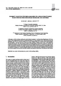
Figure 4,
Frequency
response plots for actual plant, G, nominal
plant, Go, and (G – Go).
/
;,.
,
,Nmmlmxl f:rcqwmcb,
Figure 5.
Frequency
response plots of actual plant and its reduced order approximations.
This controller also stabilizes the actual plant G. The transfer function s is then computed via (2.17). Its gain verses normalized frequency plot is shown in Fig. 6. ModeI reduction through balanced truncation is again used to find a low-order model approximation to ,S,The frequency response of a sixth order reduced model is shown alongside the frequency response of S. From these plots (and phase plots) it is immediate that the degree of fit of the sixth-order reduced model for S is comparable to the tenth-order approximation for the actual plant G and is superior compared to the sixth-order approximation of the actual plant.
Fixed
controller
1951
enhancement
performance
I ,:
Nmmlmd
Figure6.
Frequency
Frequency
response plots of full order Sand
reduced order S.
3.
Identification lt was shown in the last section that there are advantages in using the S parametrization to model the deviation of the actual plant G from the nominal plant GO. In this section, we investigate ways in which S can be conveniently identified online. Lemma
3.1
Consider a nominal plant GO and a stabilizing controller KO with coprime fiactorizations (2.3) and (2.5) satisfying the Bezout identity of (2.6). Consider Fig, 7 with G parametrized by S of (2.14) and JK given by (2.11). Under the above conditions, the transfer function matrix from [w\ w’> s’]’ to [e\ e: r’]’ of Fig. 7 is given by [ w=
(J– [
where
(l– KOG)-’KO
(,-KOG)-l GKO)-lG
V; ’(l–
S is given from
GKO)-l
(l–
(l–
GKo)”
(l–
G
V; ’(l– GKO)-L
a“
[
KoG)-l~;’ GKO)-’G~;’
s
(2. 14),
w
‘b-L-J’
I
(h)
L-J
(,1) Figure 7.
Non-nominal
plant case
(3.1) 1
T. T. Tay et al.
1952 Proof’
From
Fig. 7, simple manipulations
w =
(l–
GKO)-l G
(l–
GK())-’G
V;l([–
V; ’(l–
[ Now
(l– K,, G)-’K()
K,, G)-’
([–
utilizing
the double
V;l(I–
show that W is given by
GK())
Bezout
GK,))-’ GKO)-l identity
VO1(I (2.6) and
‘lG~;l–V;lN(l=~~;’–V;’N() [1
=( NO+,SPO)V; ’– V; ’N(, =S Remark
8
The key message to the output r and s,
of this lemma is that the transfer
r is ,S.Thus information
function
about S can be deduced
matrix
from the input
by observing
,s
the signals
To formulate the identification of S into the framework ofa standard identification algorithm, it is necessary to adopt some kind of noise model. Let us assume that the actual plant has a general associated noise model as given in Fig. 8(u). Here w is a noise sequence and Gw,is the filter associated with the noise. Simple manipulations show that Fig. 8((/) c:in be redrawn as Fig. 8(h) with (3.3)
r = S,s + A7Gww
‘i
1’
((/)
Figure 8.
Piant) noise model.
This turns out to bc a linear eauation in Yand can easily bc reformulated into forms so that a standard identification algorithm such as the recursive least squares or extended least squares can be applied. The noise tiltcr ( fiGM, ) will depend on the appropriate G., defining the underlying noise process,
.E.Yun?plP 2
Let us demonstrate the above for the case where the underlying a scalar AR MAX description G=
B(z-’)/A(z-’),
A(z-’)=l+alz-’
c(z-’)=
l+clz-~+...
actual process has
GW,=C(~-l)/A(z-l) +..,+~l~~-m,
+cp:-’
B(~-l)=
bO+blz-
l+,,,
( 3.4)
+h,, z-” 1
Fixed Assume
that
a nominal
perfiwnunce
controller
plant
Go is available
and
1953
~nhuncemenf Go is given
by
Go= Bo(:-’)/AO(z-l)
1
1+... +(imom0,0, Bo(z-i) =bo+filZ-l+. ..+hoZ
,40= l+tiizLet the factorization
/7
(J.J)
for G and Go be given by
Alo=
MO=
J
–nO
1), NO=N[) =Bo[z’l)/Do(z-l)
/40(z-1)/Do(z-
.M=fi=A(:-
l)/D(z-’),
N=~=B(z-l)/D(z-’)
1
where D(z - 1) and D[)(z -1 ) are stable polynomials derived from the Pactorizations (2.7), (2.23) or (2.24). Now let us assume that S is parametrized by polynomials As(.z - 1), Bs(z’1 )
(3.6)
of
(3.7)
S== BS(Z-l)/AJ-l) Then from (2. 17), wc have A$(z ‘l)= MGM,
D(Z-l)Do(:-
l),
=CtZ-’)/D(Z-l),
)=
BS(~-’
C’S(Z
-’)
B(z-’)Ao(z-’
=C(Z-l)DO(Z-’) 1 I I
and As(z-’)r
A(z()Bo(zo)z-’)
=Bs(z-’)s
J
+Cs(”l)w)w
and the extended
can be used to estimate As(z -1 ) and from the factorization of (2.7), (2.23) or (2.24), DO(Z- 1) ret3ects the nominal closed-loop poles and can be appropriately designed through the design of the nominal controller K.. Bs(z-’
) on-line.
least squares
(3.8)
Given
that
algorithm
Do(z - 1) is derived
Control Identification of S through the scheme of $3 is a first stage which is interesting in its own right and may find applications in process identification where it is desirable to combine physical structure/parameters determination with algorithmic techniques like least squares. However a logical next stage is to exploit the on-line estimation of S for an on-line enhancement of controller performance. This aspect is now explored. We shall make a brief note on the closed-loop stability of our on-line adaptive scheme before going on to describe possible utilization of the information provided by S. 4.
4,1. Closed-1oop
stobilit~,
The objective of the adaptive scheme is to enhance performance by adapting Q, now denoted Q~, and thereby achieving an adaptive controller K(Q~) for the plant G(S). Of course, the first requirement is stabilization. From the theory of\ 2, we are able to view the original problem of adapting K(Q~) for G(S) to achieve stability as the derived problem of adapting the ‘controller’, Q~ to stabilize the ‘plant’, S, now a standard task. This is depicted in Fig. 9. We shall next describe two adaptive algorithms for tuning the ‘controller’, Q~. We stress here that the algorithms to be described are not new. Rather, what we aim to achieve in the following part of this section is to justify the use of these algorithms to achieve our control objectives, whether these be merely stabilization, or poleplacement, or linear quadratic control.
T, T. Tay et al.
1954
‘--Q-+ * (