Induction Motor Fault Diagnostic and Monitoring Methods

INDUCTION MOTOR FAULT DIAGNOSTIC AND MONITORING METHODS

by

Aderiano M. da Silva, B.S. A Thesis submitted to the Faculty Of the Graduate School, Marquette University, In Partial Fulfillment of the Requirements for the Degree of Master of Electrical and Computer Engineering Milwaukee, Wisconsin May 2006

i

Abstract Induction motors are used worldwide as the “workhorse” in industrial applications. Although, these electromechanical devices are highly reliable, they are susceptible to many types of faults. Such fault can became catastrophic and cause production shutdowns, personal injuries, and waste of raw material. However, induction motor faults can be detected in an initial stage in order to prevent the complete failure of an induction motor and unexpected production costs. Accordingly, this thesis presents two methods to detect induction motor faults. The first method is a motor fault diagnostic method that identifies two types of motor faults: broken rotor bars and inter-turn short circuits in stator windings. These two types of faults represent 40 to 50% of all reported faults. Moreover, this method identifies the motor fault’s severity through the identification of the number of broken bars and the number of turns involved in an interturn short. The second method is a motor fault monitoring method that classifies the operating condition of an induction motor as healthy or faulty. The faulty condition represents any number of broken bars. This method has two major advantages. First, this is a robust technique, which is trained with datasets generated by time-stepping finite element methods in order to monitor faults of real induction motors in operation. Thus, the high cost associated with destructive tests to generate the training sets is not required. Second, it will be demonstrated here that this method, which is trained with simulated data of only one motor, can be used to monitor faults of real motors even with different design specifications. This establishes the scalability of this method. Both methods are validated through experimental tests.

ii

Acknowledgement

Special thanks for my advisor Dr. Richard J. Povinelli for his teaching, support and encouragement during the development of this research. Special thanks for Dr. Nabeel A. O. Demerdash for his teaching, reviews and discussions during this research. Special thanks for Dr. Edwin E. Yaz for his teaching, support and discussions during this research. Finally, I would like to thanks my wife Marcia Silva for her support and motivation during this time, and also for my little daughter Nicole Silva for her smiles. This material is based upon work supported by the US National Science Foundation under Grant No. ECS-0322974.

iii

Table of Contents

CHAPTER 1

INTRODUCTION ........................................................................................... 1

1.1

LITERATURE REVIEW ........................................................................................... 4

1.2

NEW METHODS .................................................................................................... 7

1.2.1

Induction motor fault diagnostic method.................................................... 8

1.2.2

The induction motor fault monitoring method ............................................ 9

1.3

ORGANIZATION OF THE THESIS .......................................................................... 10

CHAPTER 2 2.1

BACKGROUND ........................................................................................... 12

INDUCTION MOTORS .......................................................................................... 12

2.1.1

Induction motor components..................................................................... 14

2.1.2

Induction motor operation ........................................................................ 17

2.1.3

Parameters of induction motors................................................................ 20

2.2

AC DRIVES ........................................................................................................ 31

2.3

INDUCTION MOTOR FAULTS .............................................................................. 37

2.3.1

Broken rotor bars...................................................................................... 38

2.3.2

Inter-turn short circuits............................................................................. 39

2.4

INDUCTION MOTOR FEATURES USED IN THE DIAGNOSTIC AND MONITORING

METHODS ...................................................................................................................... 43 2.4.1

The three-phase stator current envelope .................................................. 44

2.4.2

The air gap torque profile......................................................................... 47

iv

CHAPTER 3

INDUCTION MOTOR FEATURES AND AI TECHNIQUES ............................ 50

3.1

THE AIR GAP TORQUE OBSERVER ..................................................................... 51

3.2

THE SPEED OBSERVER ....................................................................................... 57

3.3

THE RECONSTRUCTED PHASE SPACE ................................................................. 66

3.4

THE GAUSSIAN MIXTURE MODELS .................................................................... 77

CHAPTER 4

METHODOLOGY........................................................................................ 81

4.1

THE TRAINING AND TESTING STAGES ................................................................ 84

4.2

THE INDUCTION MOTOR FAULT DIAGNOSTIC METHOD ..................................... 89

4.3

THE INDUCTION MOTOR FAULT MONITORING METHOD .................................... 95

CHAPTER 5

EXPERIMENTAL VERIFICATION OF THE PRESENTED METHOD ............ 105

5.1

RESULTS FOR THE INDUCTION MOTOR FAULT DIAGNOSTIC METHOD ............. 105

5.2

DISCUSSION OF RESULTS FOR THE INDUCTION MOTOR FAULT DIAGNOSTIC

METHOD ...................................................................................................................... 115 5.3

RESULTS FOR THE INDUCTION MOTOR FAULT MONITORING METHOD ............ 120

5.4

DISCUSSION OF RESULTS FOR THE INDUCTION MOTOR FAULT MONITORING

METHOD ...................................................................................................................... 123 CHAPTER 6

CONCLUSIONS ......................................................................................... 127

BIBLIOGRAPHY ............................................................................................................... 130 APPENDIX A.................................................................................................................... 142

v

List of Tables

Table 1.1 - Percentage of failure by component ................................................................. 3 Table 3.1 - Speed estimated by a speed observer for a 2-hp, 2-pole, induction motor..... 65 Table 5.1 - Accuracy of fault classification for a 5-hp, 6-pole, induction motor with one through four broken bars at 60 Hz and three different motor loads based on a testing set with 50 samples. ......................................................................... 109 Table 5.2 - Accuracy of fault classification for a 5-hp, 6-pole, induction motor with one through four broken bars at 40 and 60 Hz based on a testing set with 30 samples. The test was carried out at rated load. .......................................... 111 Table 5.3 - Accuracy of fault classification for a 5-hp, 6-pole, induction motor with one through four inter-turn short-circuits in the stator windings at frequency of 60 Hz and motor loads of 50, 75 and 100% of the rated torque based on a testing set with 50 samples...................................................................................... 113 Table 5.4 - Accuracy of fault classification for a 5-hp, 6-pole, induction motor with one through four broken bars or one through four inter-turn short-circuit in stator windings at frequency of 60 Hz and motor loads of 50, 75 and 100% of the rated torque based on a testing set with 90 samples.................................... 114 Table 5.5 - Confusion matrix for the 99% classification accuracy of the 5-hp, 6-pole, induction motor with one through four broken bars or one through four interturn short-circuit in stator windings at frequency of 60 Hz and motor loads of

vi

50, 75 and 100% of the rated torque based on a testing set of 90 samples and with 32 fault signature mixtures. ................................................................. 115 Table 5.6 - Motor fault monitoring accuracy for a 2-hp, 2-pole and a 5-hp, 6-pole, 60-Hz induction motors at a frequency of 60Hz and motor loads of 50, 75 and 100% of the rated torque........................................................................................ 122

vii

List of Figures Fig. 2.1 - Types of electric motors.................................................................................... 13 Fig. 2.2 – A typical 3-phase induction motor [Courtesy of Electromotors WEG SA, Brazil]............................................................................................................... 15 Fig. 2.3 – A rotor of a squirrel cage induction motor ....................................................... 16 Fig. 2.4 – A two-pole induction motor schematic ............................................................ 17 Fig. 2.5 – The rotating magnetic field of a two-pole induction motor. The bold dots and bold plus markings represent the phase currents during peaking instants. The normal dots and plus markings represent the phase currents with amplitudes equal to half of the peak value.......................................................................... 19 Fig. 2.6 – The phasors of the three-phase stator currents and voltages of an induction motor. ............................................................................................................... 22 Fig. 2.7 – An RL series circuit.......................................................................................... 26 Fig. 2.8 – An RL series circuit supplied by two phases.................................................... 28 Fig. 2.9 – Torque applied to a shaft .................................................................................. 30 Fig. 2.10 – A typical induction motor torque-speed (torque-slip)characteristic curve..... 31 Fig. 2.11 – A functional block diagram of an ac drive ..................................................... 32 Fig. 2.12 – A circuit schematic diagram of an ac drive .................................................... 33 Fig. 2.13 – The PWM control signal and phase Va voltage. ............................................ 34 Fig. 2.14 – Typical phase voltages Va and Vb, and line voltage Vab of a PWM inverter with carrier frequency of 1 kHz and fundamental component of 60Hz........... 35 Fig. 2.15 – Typical curve of torque-speed control of an induction motor-drive system .. 36

viii

Fig. 2.16 – Typical insulation damage leading to inter-turn short circuit of the stator windings in three-phase induction motors. (a) Inter-turn short circuits between turns of the same phase. (b) Winding short circuited. (c) Short circuits between winding and stator core at the end of the stator slot. (d) Short circuits between winding and stator core in the middle of the stator slot. (e) Short circuit at the leads. (f) Short circuit between phases. [Courtesy of Electromotors WEG SA, Brazil]............................................................................................................... 40 Fig. 2.17 - Inter-turn short circuit of the stator winding in three-phase induction motors. (a) Short circuits in one phase due to motor overload (b) Short circuits in one phase due to blocked rotor. (c) Inter-turn short circuits are due to voltage transients. (d) Short circuits in one phase due to a phase loss in a Y-connected motor. (e) Short circuits in one phase due to a phase loss in a delta-connected motor. (f) Short circuits in one phase due to an unbalanced stator voltage. [Courtesy of Electromotors WEG SA, Brazil]................................................. 42 Fig. 2.18 - One slip cycle of the three phase stator current envelope for a three-phase, 460V, 60-Hz, 6-pole, 5-hp squirrel-cage induction motor with four broken bars under rated load. ............................................................................................... 45 Fig. 2.19 - Three phase stator current envelope for a three-phase, 460V, 60-Hz, 6-pole, 5hp squirrel-cage induction motor with four inter-turn short circuits under rated load. .................................................................................................................. 46 Fig. 2.20 – Air gap torque profile for a three-phase, 460V, 60-Hz, 6-pole, 5-hp squirrelcage induction motor with four broken bars under rated load, at 1165r/min... 48

ix

Fig. 3.1 – Pseudo-code of the air gap torque observer...................................................... 54 Fig. 3.2 – Air gap torque profile for a three-phase, 460V, 60-Hz, 2-pole, 2-hp squirrelcage induction motor with five broken bars under rated load simulated by finite element method. ............................................................................................... 56 Fig. 3.3 - Air gap torque profile for a three-phase, 460V, 60-Hz, 2-pole, 2-hp squirrelcage induction motor with five broken bars under rated load calculated by the air gap torque observer using the three-phase stator currents and voltages obtained from the simulation............................................................................ 56 Fig. 3.4 – Error between the air gap torque obtained from finite element simulations and the air gap torque calculated by the torque observer using the three-phase stator and currents obtained from the simulations. .................................................... 57 Fig. 3.5 – Power spectrum of the stator current of a three-phase, 2-hp, 2-pole, squirrel cage induction motor running at 80% of rated torque...................................... 63 Fig. 3.6 – Power spectrum of the window [2010Hz, 2100Hz] for the stator current of a three-phase, 2-hp, 2-pole, squirrel cage induction motor running at 80% of rated torque....................................................................................................... 64 Fig. 3.7 – Stator current sampled at 1kHz. ....................................................................... 67 Fig. 3.8 – Normalized stator phase current of the 460-V,6-pole, 5-hp induction motor with four broken bars. ...................................................................................... 70 Fig. 3.9 – Automutual information of the stator phase current for the 460-V, 6-pole, 5-hp induction motor with four broken bars............................................................. 70

x

Fig. 3.10 – False nearest neighborhood of the of the stator phase current for the 5-hp induction motor with four broken bars............................................................. 73 Fig. 3.11 – Reconstructed phase space of the phase stator current of the 5-hp induction motor with four broken bars............................................................................. 74 Fig. 3.12 – RPS of the three-phase envelope of the 460-V, 2-pole, 2-hp induction motor with one broken bar with τ = 5......................................................................... 75 Fig. 3.13 - RPS of the air gap torque of the healthy 2-hp induction with τ = 20.............. 76 Fig. 3.14 – The full covariance matrix model................................................................... 79 Fig. 4.1 – The algorithm of the presented method. (a) Training stage. (b) Testing or classification stage............................................................................................ 86 Fig. 4.2 – The Gaussian mixture model of the three phase stator current envelope of the 460-V, 6-pole, 5-hp faulty induction machine reconstructed phase space with eight (8) mixtures, dimension two (2) and time lag nine (9)............................ 88 Fig. 4.3 - Algorithm of the induction motor diagnostic method. (a) Training stage. (b) Testing or classification stage .......................................................................... 91 Fig. 4.4 – The process of obtaining the three-phase stator current envelope. (a) Threephase stator current. (b) Ripple of the three-phase stator current. (c) Filtered ripple. (d) Envelope identification. (e) Interpolation of the envelope. (f) Normalization of the envelope. ........................................................................ 92 Fig. 4.5 – The high level algorithm of the monitoring method......................................... 95 Fig. 4.6 – Detailed algorithm for the induction motor fault monitoring method.............. 96

xi

Fig. 4.7 – The process of obtaining the air gap torque profile for the training stage of the monitoring method for the 2-hp induction motor at 60Hz and rated torque with one broken bar simulated by finite elements software. (a) Air gap torque from the MAGSOFT. (b) Torque without dc offset. (c) Filtered torque signal. (d) Filtered and normalized torque signal. ............................................................. 98 Fig. 4.8 – The process of obtaining the air gap torque profile for the testing stage of the monitoring method for the 5-hp motor at rated speed and load torque. (a) Air gap torque obtained from a torque observer. (b) Air gap torque without dc offset. (c) Filtered air gap torque signal without dc offset. (c) Air gap torque profile after the frequency normalization process.......................................... 101 Fig. 4.9 - Air gap torque profile of the 6-pole, 60Hz, 5-hp motor with 4 broken bars in which TRM is shown in one slip cycle............................................................. 102 Fig. 5.1 - Laboratory test setup for a 5-hp induction motor data acquisition. ................ 106 Fig. 5.2 - The schematic of stator winding tappings for the tested induction motors..... 107

Chapter 1: Introduction

1

CHAPTER 1 Introduction Chapter 1

I

Introduction

NDUCTION MOTORS are complex electro-mechanical devices utilized in most industrial applications for the conversion of power from electrical to

mechanical form. Induction motors are used worldwide as the workhorse in industrial applications. Such motors are robust machines used not only for general purposes, but also in hazardous locations and severe environments. General purpose applications of induction motors include pumps, conveyors, machine tools, centrifugal machines, presses, elevators, and packaging equipment. On the other hand, applications in hazardous locations include petrochemical and natural gas plants, while severe environment applications for induction motors include grain elevators, shredders, and equipment for coal plants. Additionally, induction motors are highly reliable, require low maintenance, and have relatively high efficiency. Moreover, the wide range of power of induction motors, which is from hundreds of watts to megawatts, satisfies the production needs of most industrial processes.


2

However, induction motors are susceptible to many types of fault in industrial applications. A motor failure that is not identified in an initial stage may become catastrophic and the induction motor may suffer severe damage. Thus, undetected motor faults may cascade into motor failure, which in turn may cause production shutdowns. Such shutdowns are costly in terms of lost production time, maintenance costs, and wasted raw materials. The motor faults are due to mechanical and electrical stresses. Mechanical stresses are caused by overloads and abrupt load changes, which can produce bearing faults and rotor bar breakage. On the other hand, electrical stresses are usually associated with the power supply. Induction motors can be energized from constant frequency sinusoidal power supplies or from adjustable speed ac drives. However, induction motors are more susceptible to fault when supplied by ac drives. This is due to the extra voltage stress on the stator windings, the high frequency stator current components, and the induced bearing currents, caused by ac drives. In addition, motor over voltages can occur because of the length of cable connections between a motor and an ac drive. This last effect is caused by reflected wave transient voltages [1]. Such electrical stresses may produce stator winding short circuits and result in a complete motor failure. According to published surveys [2, 3], induction motor failures include bearing failures, inter-turn short circuits in stator windings, and broken rotor bars and end ring faults. Bearing failures are responsible for approximately two-fifths of all faults. Interturn short circuits in stator windings represent approximately one-third of the reported faults. Broken rotor bars and end ring faults represent around ten percent of the induction


3

motor faults. These faults are summarized in Table 1.1. This table presents the surveys conducted by the Electric Power Research Institute (EPRI), which surveyed 6312 motors [3], and the survey conducted by the Motor Reliability Working Group of the IEEE-IAS, which surveyed 1141 motors [2].

Table 1.1 – Percentage of failure by component Failed Component Bearings Related Windings Related Rotor Related Others

Percentage of failures (%) IEEE-IAS EPRI 44 41 26 36 8 9 22 14

Several alternatives have been used in industry to prevent severe damage to induction motors from the above mentioned faults and to avoid unexpected production shutdowns. Schedule of frequent maintenance is implemented to verify the integrity of the motors, as well as to verify abnormal vibration, lubrication problems, bearings conditions, and stator windings and rotor cage integrity. Most maintenance must be performed with the induction motor turned off, which also implies production shutdown. Usually, large companies prefer yearly maintenance in which the production is stopped for full maintenance procedures. Redundancy is another way to prevent production shutdowns, but not induction motor failure. Employing redundancy requires two sets of equipment, including induction motors. The first set of equipment operates unless there is a failure, in which case the second set takes over. This solution is not feasible in many


4

industrial applications due to high equipment cost and physical space limitations. Thus, in this thesis an alternative to these approaches is proposed. Specifically, this thesis addresses electrically detectable faults that occur in the stator windings and rotor cage, namely inter-turn short circuits in stator windings and broken rotor bars. The methods developed in this thesis detect motor faults without the necessity of invasive tests or process shutdowns. Moreover, the presented methods monitor the operating induction motor continuously, so that human inspection is not required to detect motor faults. Now that the central problem of this thesis has been presented, a literature review about motor fault identification methods including their advantages and disadvantages is made.

1.1

Literature Review Significant efforts have been dedicated to induction machine fault diagnosis

during the last two decades and many techniques have been proposed [4-32]. Thus, a brief description of the main techniques presented in the literature, as well as their advantages and disadvantages are presented in this section. Several fault detection and identification techniques are based on stator current spectral signature analysis, which uses the power spectrum of the stator current [10, 20] to detect broken rotor bar faults. These fault detection techniques are based on the magnitude of certain frequency components of the stator currents. Specifically, a Fast Fourier Transform (FFT) of the current is taken. The first spectral peak less than the


5

fundamental frequency is called the low sideband. The magnitude of the low sideband is measured and compared to a threshold. The result of this comparison determines if an induction motor has broken rotor bars. However, these techniques may fail to detect induction motor fault conditions because the sidebands can be masked due to the windowing processes used to compute the power spectrum of the current signals, as was shown in [27]. The analysis of the negative sequence components of the stator current is another well-know technique used to detect inter-turn short circuits [21, 22]. This technique is based on the detections of the asymmetries produced by a faulty motor with shorted turns in the stator winding. Such asymmetries will generate a negative sequence current, which is used to detect the fault. A negative sequence is derived from a vectorial interpretation of unbalanced three phase currents or voltages [33]. For an induction motor, an unbalanced 3-phase stator current can be decomposed as a balanced 3-phase positive sequence (ABC) and a balanced 3-phase negative sequence (ACB). Moreover, the magnitude of the negative sequence current is proportional to the magnitude of the unbalanced effect of the induction motor. Thus, balanced motors have only positive sequences. However, some effects can yield misclassification, such as unbalanced power supply voltage, certain types of load, and instrument errors, because such effects produce negative sequence currents even in healthy motors. Such effects were considered in [21]. However, this method still fails to detect faults for induction motors with inherently unbalanced windings, as was shown in [26].


6

Other techniques include vibration analysis, acoustic noise measurement, torque profile analysis, temperature analysis, and magnetic field analysis [28, 30]. These techniques require sophisticated and expensive sensors, additional electrical and mechanical installations, and frequent maintenance. Moreover, the use of a physical sensor in a motor fault identification system results in lower system reliability compared to other fault identification systems that do not require extra instrumentation. This is due to the susceptibility of the sensor to fail added to the inherent susceptibility of the induction motor to fail. Recently, new techniques based on artificial intelligence (AI) approaches have been introduced, using concepts such as fuzzy logic [32], genetic algorithms [28], and Bayesian classifiers [18, 34]. The AI-based techniques can not only classify the faults, but also identify the fault severity. These methods build offline signatures for each motor operating condition and an online signature for the status of a motor being monitored. A classifier compares the previously learned signatures with the signature generated online in order to classify the motor operating condition and identify the fault severity. However, most of these AI-based techniques require large datasets. These dataset are used to learn a signature for each motor operating condition that is being considered for classification. Thus, a large amount of data is needed to train such algorithms in order to cover the most common motor operating conditions, and obtain good motor fault classification accuracy. Moreover, AI-based techniques for motor fault classification may not be sufficiently robust to classify faults from different motors from those used in the


7

training process. Additionally, these datasets are usually not available, involve destructive testing, and considerable time to generate. Additionally, a method using the motor internal physical condition based on a socalled pendulous oscillation of the rotor magnetic field space vector orientation has been introduced for motor fault classification [7, 25, 27]. This technique classifies the faults and identifies the fault severity of induction motors with broken rotor bars or inter-turn short circuit. However, this index identification based technique needs to evaluate each new motor to obtain the correct set of indexes in order to correctly classify the faults. The two new methods for motor fault classification and monitoring that are the subject of this thesis are briefly introduced in the next section.

1.2

New Methods This thesis presents two new methods. The first method is an induction motor

fault diagnostic technique, which classifies two types of motor faults: broken rotor bars and inter-turn short circuits. Additionally, this method identifies the motor fault severity. This method will be referred to as the diagnostic method throughout the thesis. The second method is an induction motor fault monitoring technique which classifies the operating condition of an induction motor as faulty or healthy. This second method is a robust technique, because it can be trained with datasets generated by Finite Element methods and monitors the faults of real induction motors independently of their power ratings, number of poles, level of load torque, and operating frequency. This robustness is


8

demonstrated experimentally in Chapter 5. The second method is referred to as the monitoring method throughout the thesis.

1.2.1 Induction motor fault diagnostic method The method presented in this thesis for induction motor fault diagnosis is based on the analysis of the envelope of the three phase stator current. This diagnostic method can classify two types of induction motor faults: broken rotor bars and inter-turn short circuits in the stator windings. Experimental results show that the three phase current envelope is a powerful feature for motor fault classification. The envelope signal is extracted from the experimentally acquired stator current signals and is used in conjunction with machine learning techniques based on Gaussian Mixture Models [34] (GMMs) and Reconstructed Phase Spaces (RPSs) [34-36] to identify motor faults. In addition, this diagnostic method not only classifies an induction motor as healthy or faulty, but also identifies the severity of the fault through the identification of the number of broken rotor bars or the number (or percentage) of short-circuited turns in stator windings. This constitutes a powerful means of monitoring motor fault severities, which could possibly predict the time of onset of complete failure of a motor, and thus help prevent unexpected shutdowns of industrial processes. The second advantage of this method is that the classification process needs only the three-phase stator current sensors, usually available in ac drives. Thus, extra electrical and mechanical installations, sensors, and mathematical models of an induction motor are not required.


9

1.2.2 The induction motor fault monitoring method The second method presented in this thesis is an induction motor fault monitoring technique based on the air gap torque profile analysis, associated with machine learning techniques to classify the operating condition of an induction motor as healthy or faulty. These machine learning techniques are based on GMMs and RPSs. The important novel nature of this approach is two-fold. First, the necessary healthy and faulty motor signatures to train this method are obtained from finite element simulations, not from experimental data. Second, the signatures can be applied to different classes of induction motors through a novel normalization process. A faulty condition represents any number of broken rotor bars. The signatures used in the training stage are based on the air gap torque profile of an induction motor simulated by a time-stepping Finite Element method. In the monitoring stage a new signature is built for the developed torque. This torque is calculated online from a new set of three-phase stator voltages and currents acquired from an actual induction motor being monitored. A comparison of the signatures obtained at the training and monitoring stages classifies the motor operating condition. This monitoring method has two main advantages. The first advantage is the robustness of the monitoring processes, in which the training stage uses data generated by finite element simulations, in order to monitor the operating conditions of real induction motors during the actual operating (monitoring) stage. This is accomplished with high levels of motor fault monitoring accuracy, as shown by the experimental results given in Chapter 5. It should be pointed out that the training process is performed offline, while the monitoring process is performed online. These training and monitoring processes


10

based on data from different sources (simulations and real motors operating data, respectively) show the robustness of the method. Thus, high costs associated with equipment to emulate the faults or destructive tests to generate datasets to train this method are not involved. The second advantage is related to scalability of the monitoring process. The signatures for the training and monitoring stages are normalized in amplitude. However, the signatures of the monitoring stage are not only normalized in amplitude, but also in frequency. This normalization in frequency of the signatures of the monitoring stage is a function of the signatures of the training stage. Thus, the signatures from the training and monitoring stages for the same motor operating condition have similar amplitude and frequency. These signatures with similar amplitude and frequency for the same motor operating condition are essential in the monitoring stage to yield high level of motor fault monitoring accuracy. Accordingly, the training and monitoring stages yield signatures that are independent of motor rated power, number of poles, level of load torque, and operating frequency of the real motor that is being monitored. Thus, this method constitutes a powerful tool for induction motor fault monitoring. This is demonstrated and verified by the experimental results given in Chapter 5 of this thesis.

1.3

Organization of the Thesis The remainder of this thesis is organized as follows. Chapter 2 presents the

necessary background concerning induction machines and ac drives, as well as a discussion of induction motor faults. Chapter 3 details the features of induction motors


and machine learning techniques used in the new diagnostic method and the new monitoring method presented in this thesis. Chapter 4 presents the new fault diagnostic method and the new fault monitoring method. Chapter 5 presents experimental verification of the new methods and an overall discussion of the results. Chapter 6 presents the conclusions.

11

Chapter 2: Background

Chapter 2

12

Background

CHAPTER 2 Induction Motor and AC Drive This chapter presents a basic description of the physical phenomena related to induction motors, ac drives, and induction motor faults. Moreover, it explains the physical phenomena of faulty induction motors with either broken rotor bars or inter-turn short-circuits in the stator windings.

2.1

Induction Motors Induction motors are complex electro-mechanical devices used worldwide in

industrial processes to convert electrical energy into mechanical energy. Such motors are widespread because they are robust, easily installed, controlled, and adaptable for many industrial applications, including pumps, fans, air compressors, machine tools, mixers, and conveyor belts, as well as many other industrial applications. Moreover, induction motors may be supplied directly from a constant frequency sinusoidal power supply or by an ac variable frequency drive. These drives are discussed in the Section 2.2.


13

Different types of electric motors are illustrated in Fig. 2.1 [37].

Fig. 2.1 - Types of electric motors.


14

Due to the large range of types and applications of electric motors, the focus of this discussion will be on those studied in this thesis. In other words, the focus is on the three-phase squirrel cage induction motor, which is a type of asynchronous motor. As is common in the literature, a three-phase squirrel cage induction motor is referred to as an induction motor throughout this thesis. This type of induction motor is highlighted in Fig. 2.1 in grey. The following section illustrates the main components of an induction motor.

2.1.1 Induction motor components Although an induction motor has several parts as shown in Fig. 2.2, it is essentially composed of a squirrel cage rotor and a wound stator [38]. The rotor is composed of a squirrel cage, a shaft, and a lamination stack as shown in Fig. 2.3. The main part of the rotor is the squirrel cage, which is composed of bars and two end rings. The conductive rotor bars are short-circuited on both sides by the end rings. Thus, the electric current can circulate from one side to other side of the squirrel cage. The bars are enveloped by a laminated iron core, which concentrates the magnetic flux from the stator windings in the rotor. This lamination also mechanically supports the rotor shaft. The bearings on both sides of the rotor shaft allow the rotor to spin freely inside the stator.


15

Fig. 2.2 – A typical 3-phase induction motor [Courtesy of Electromotors WEG SA, Brazil] The stator is composed of three parts: frame, lamination core and windings. The frame mechanically supports the stator and the rotor shaft bearings. The windings are composed of three equally distributed coils along the stator lamination core, which are connected to the three-phase power supply. Only the stator is connected to the power supply. The energy for the rotor is delivered by induction by the synchronous rotation of the stator magnetic field. The name of the “induction motor” is thus derived from this phenomenon. It should be pointed out that there is a space between the stator and the rotor which is called the air gap.


Fig. 2.3 – A rotor of a squirrel cage induction motor

16


17

2.1.2 Induction motor operation The operating principle of an induction motor is thus based on the synchronously rotating magnetic field [39]. The stator is composed of three windings electrically shifted 120ºe as shown in Fig. 2.4. The three windings are connected to a three phase ac power supply.

Fig. 2.4 – A two-pole induction motor schematic When a current, I, pass through a coil, it induces a magnetic field with two poles (north and south) in this coil. The generated magnetic field H is proportional to the current I. The magnetic field H has a sinusoidal spatial distribution characteristic, and inverts polarity each half period of 180°e. Thus, three magnetic fields, HA, HB, and HC, B

are generated when the three phase stator current, IA, IB, and IC, are applied to the stator B


18

windings. The 120ºe phase-shift of the three phase stator currents yield a 120ºe phaseshift on the three magnetic fields, HA, HB, and HC. The path of these magnetic fluxes is B

through the rotor and the stator laminations. The resulting magnetic field at each time instant is equivalent to the sum of the magnetic fields, HA, HB, and HC, at that specific B

time instant. The resulting magnetic field rotates as shown in Fig. 2.5. The time instant one (1) of the three phase stator current shown in Fig. 2.5 yields a maximum magnetic field HA due to the peak value of phase current A, and a magnetic field HB and HC with B

amplitude equal to a half of the maximum value. The resulting magnetic field for this time instant has the direction of HA. In a similar manner, this same process is repeated for the other time instants two (2) though six (6), yielding a synchronously rotating magnetic field with constant peak amplitude. Thus, this rotating magnetic field generated by the three phase currents applied to the stator windings induces electrical currents in the rotor bars, when the magnetic flux from the stator cuts across the rotor bars. These rotor currents generate a magnetic field on the rotor with opposite polarity in relation to the stator. Since opposite poles attract, the rotor follows the rotating magnetic field of the stator resulting in a rotation of the rotor slightly slower than the rotating magnetic field of the stator. This difference in rotational speed between the rotating fields of the stator and rotor bars is called the slip speed, which will be discussed next in this chapter. In order to produce the required torque, only a small slip speed is required to produce the necessary rotor current due to the small resistance of the shorted rotor bars [40]. Thus, the rotor develops a torque proportional to the product of the stator and rotor currents.


19

Fig. 2.5 – The rotating magnetic field of a two-pole induction motor. The bold dots and bold plus markings represent the phase currents during peaking instants. The normal dots and plus markings represent the phase currents with amplitudes equal to half of the peak value.


20

2.1.3 Parameters of induction motors This section defines several well-known parameters of induction motor used in the remainder of this thesis. 2.1.3.1

Voltage and current An induction motor is supplied by a three-phase ac system in which the three-

phase currents are phase-shifted by 120ºe or 2π/3 electrical radians. The three phase currents are thus defined as (2.1)[39]. ia = I m cos (ωt − φ ) 2π ⎞ ⎛ ib = I m cos ⎜ ωt − φ − ⎟ 3 ⎠ ⎝ 2π ⎞ ⎛ ic = I m cos ⎜ ωt − φ + ⎟, 3 ⎠ ⎝

(2.1)

where ia is the current in phase A, ib is the current in phase B, ic is the current in phase C, Im is the peak fundamental frequency value of each phase current, ω is the fundamental electrical angular frequency in (rad/s), φ is the lag power factor angle in e.rad, and t is time (s). Due to the symmetric phase-shift of 120ºe in the phase currents, the sum of the three phase currents is zero as given by (2.2).

ia + ib + ic = 0.

(2.2)


21

The phase voltages are also phase-shifted by 120ºe or 2π/3 e.rad. Considering the phase voltage, va, as reference, the three phase voltages are defined as (2.3).

va = Vm cos (ωt ) 2π ⎞ ⎛ vb = Vm cos ⎜ ωt − ⎟ 3 ⎠ ⎝ 2π ⎞ 4π ⎛ ⎛ vc = Vm cos ⎜ ωt + ⎟ = Vm cos ⎜ ωt − 3 ⎠ 3 ⎝ ⎝

(2.3) ⎞ ⎟, ⎠

where, va is the phase voltage A, vb is the phase voltage B, vc is the phase voltage C, and Vm is the peak fundamental frequency value of the phase voltage. In polar form, the three phase voltages can be written as (2.4).

V a = Vm 0º V b = Vm −120º = Vm − 2π 3

(2.4)

V c = Vm −240º = Vm − 4π 3.

Again, due to the symmetric phase-shift of 120ºe in the phase voltages, the sum of the three phase voltages is zero as given by (2.5).

va + vb + vc = 0.

(2.5)

The three-phase voltage system is defined in terms of the phase voltage (vp) or the line voltage (vl). The relation between vp and vl is defined in (2.6).


22

vl = v p 3.

(2.6)

When the three-phase voltage system is applied to an induction motor, the phase currents are phase-shifted from the phase voltages in the lagging direction by the power factor angle, φ, which appears to be close to a value of 30º for the classes of 2-hp and 5hp motors studied in this thesis, as shown by the phasor diagram in Fig. 2.6, where V ab ,

V bc , and V ca are the line-to-line voltages and V a , V b , and V c are the phase voltages.

Fig. 2.6 – The phasors of the three-phase stator currents and voltages of an induction motor.


23

In this case, V ab , V bc , and V ca are given by (2.7).

V ab = V a − V b V bc = V b − V c

(2.7)

V ca = V c − V a . It should be pointed out that the peak value of the phase voltage Vm is related to the rms value of the phase voltage vrms by a factor

vrms =

1

2 as given in (2.8).

π

2 ⎡⎣Vm cos (ωt ) ⎤⎦ d (ωt ) ∫ π 0

vrms =

1

π

Vm

2

π

⎡1 ⎤ ⎢⎣ 2 (ωt − sin (ωt ) cos (ωt ) ) ⎥⎦ 0 vrms =

2.1.3.2

Vm 2

(2.8)

.

Synchronous speed, asynchronous speed, and slip speed

The speed of the magnetic rotating field is the synchronous speed. For a induction motor with P poles, the synchronous speed is given in r/min as (2.9).

nsyn =

120 f , P

where, f is the stator frequency in Hertz, and nsyn is the synchronous speed in r/min.

(2.9)


24

However, the rotor rotates at an asynchronous speed, which is slightly slower than the synchronous speed. This difference between speeds is called the slip speed and it is given as (2.10).

ns = nsys − nasyn ,

(2.10)

where, nasyn is the asynchronous speed in r/min, and ns is the slip speed in r/min. Moreover, the slip speed can also be defined in a per unit system as the slip, spu, as given in (2.11).

s pu =

nsys − nasyn nsys

.

(2.11)

As aforementioned, the synchronous speed of an induction motor connected to a constant frequency sinusoidal ac power supply depends on the frequency and number of poles. The number of poles is an inherent characteristic of an induction motor, which can be typically two, four, six, or eight, etc. On the other hand, the asynchronous rotor speed depends not only on the frequency and number of poles, but also depends of the load torque. Thus, higher torque results in a higher slip and a slower asynchronous rotor speed. Accordingly, an induction motor connected to a constant frequency sinusoidal power supply runs only at one asynchronous speed and thus provides no means of speed variation/control. In this case, an induction motor can be run only at a constant speed, and thus be used in fixed speed applications, such as pumps with constant flow, fans, air compressors, conveyor belts with constant speed, mixers, and drills.


2.1.3.3

25

Flux linkage

Flux linkage is used in electromagnetic analysis to represent the number of magnetic lines crossing an electrical circuit, such as a coil. The magnetic flux linkage ψ, is give as [41]:

ψ = ∫ Ndφ ,

(2.12)

where N is the number of turns of a coil, and φ is the magnetic flux in Weber (Wb). Thus, the flux linkage is given in Wb-turns. From Faraday’s Law, an electromagnetic force (e.m.f), e, is induced in an electrical circuit due to changes with time in the amount of flux linkage linking that circuit such that [41, 42]:

e=−

dψ . dt

(2.13)

In the same circuit, the flux linkage is proportional to the current, i. In this case, the flux linkage is given by:

ψ = Li,

(2.14)

where L is the self-inductance in Henry. Accordingly, if L is independent of i, the following relation can be derived:

e=−

d ( Li ) di dψ =− = −L . dt dt dt

(2.15)


26

That is,

dψ di =L . dt dt

(2.16)

Considering the RL series circuit in Fig. 2.7, the voltage equation given in (2.17) can be derived [43].

v = Ri + L

di dt

(2.17)

Fig. 2.7 – An RL series circuit

Algebraic manipulations yield the following new expression for flux linkage:

v = Ri + L

di dψ = Ri + . dt dt

That is,

dψ = v − Ri, dt or dψ = ( v − Ri ) dt.


27

Hence,

ψ = ∫ ( v − Ri ) dt.

(2.18)

Assuming an RL series circuit supplied by a two phase ac voltage supply as shown in Fig. 2.8, the voltages and flux linkages of phases a and b can be derived as follows:

vab = va − vb . That is, vab = R ( ia − ib ) + L vab = R ( ia − ib ) +

d ( ia − ib ) dt

d ⎡ L ( ia − ib ) ⎤⎦ . dt ⎣

Hence,

vab = R ( ia − ib ) +

dψ ab , dt

or

dψ ab d ⎡⎣ L ( ia − ib ) ⎤⎦ = = vab − R ( ia − ib ) . dt dt Accordingly,

ψ ab = ∫ vab − R ( ia − ib ) dt.

(2.19)


28

Fig. 2.8 – An RL series circuit supplied by two phases.

The same procedure can be used to obtain the so-called line-to-line flux linkages of the phases b to c, ψbc, as well as of the phases c to a, ψca, which can accordingly be written as follows, respectively:

ψ bc = ∫ vbc − R ( ib − ic ) dt.

(2.20)

ψ ca = ∫ vca − R ( ic − ia ) dt.

(2.21)

The expressions in (2.19) through (2.21) will be used in the Chapter 3 to implement a computation of the air gap torque, and hence torque observer, from measured motor terminal currents and voltages.

2.1.3.4

Magnetomotive force (mmf)

The magnetomotive force or mmf is a measure of the strength of a magnetic field. Moreover, the mmf is proportional to the number of turns in a coil and the current that flows through this coil. Thus, the measure of the mmf in a coil is the ampere-turn or just AT of that coil. Thus, 1AT represents 1A circulating in one turn of a coil. Accordingly,


29

more current implies a stronger magnetic field, and more turns also yields stronger magnetic field. In a three-phase induction motor, the fundamental mmf is given by [44]:

F1 (θ , t ) =

3 Fmax cos (θ − ωt ) 2

[AT/pole],

(2.22)

where t is time, ω is the angular frequency (velocity) in electrical radians /sec, θ is angular displacement of the rotor in electrical radians, and Fmax is the peak value of the fundamental component of the mmf, which is given by the following [44]:

Fmax =

4

π

Kw

N ph p

I 2

[AT/pole],

(2.23)

where Kw is the winding factor obtained from the electrical design of a motor, Nph is the number of series connected turns per phase, p is the number of poles, and I is the rms value of the phase current. Even in (2.23), the mmf for an induction motor is still given in terms of the number of turns times a current in a similar manner to that of a single coil. 2.1.3.5

Torque

Torque is the force needed to turn a shaft times its arm length to the axis of rotation. Thus, torque (T) is given by:

T = Fr ,

(2.24)


30

where F is the force in Newtons (N) applied to a shaft and r is the arm length of the force as shown in Fig. 2.9.

Fig. 2.9 – Torque applied to a shaft

The torque in an induction motor is produced from the interaction of the resultant air gap flux and the mmf (magnetomotive force) of either the stator winding or the rotor cage [39]. Torque is produced on the shaft of the motor only if the rotor is running at a speed lower than the synchronous speed, i.e. if the slip speed is a nonzero value. Many expressions can be used to compute the torque of an induction motor [39, 43]. Here, the following expression can be used to compute the so-called air gap torque profile [19]:

T=

p

⎡( ia − ib )ψ ca − ( ic − ia )ψ ab ⎤⎦ . 2 3⎣

(2.25)

Accordingly, substituting from (2.19) and (2.21) the following can be written for the air gap torque:

T=

p 2 3

{(ia − ib ) ∫ ⎡⎣vca − R (ic − ia )⎤⎦ dt − (ic − ia ) ∫ ⎡⎣vab − R (ia − ib )⎤⎦ dt} ,

(2.26)


31

where p is the number of poles and R is the half of the line-to-line resistance for a Yconnected motor. The first integral represents the flux linkage, ψca, of (2.21), and the second integral represents the flux linkage, ψab, of (2.19). A typical torque-speed characteristic curve of an induction motor is shown in Fig. 2.10.

Fig. 2.10 – A typical induction motor torque-speed (torque-slip)characteristic curve.

2.2

AC Drives The ac drives are electronic devices used to control speed and torque of three-

phase induction motors. An induction motor supplied by an ac drive can operate over a wide range of frequency, typically from 0 to 60Hz. This range of frequencies yields rotor speeds from 0 r/min to the rated value. Moreover, the ac drive can produce the rated torque at any frequency within this range from zero to the rated frequency. This is a


32

powerful characteristic for industrial processes that require torque-speed control. Although, the electrical installation of an ac motor-drive system is more expensive than an induction motor with a constant frequency sinusoidal power supply, the ac motordrive system can control not only the motor speed, but also can control and limit the starting torque and current, can adjust the acceleration and deceleration ramps, can maintain a constant torque for frequencies from zero to the rated frequency, and protect the motor against over voltages and over currents. The ac drives consist of three main parts, namely: three-phase full wave rectifier, dc bus filter, and pulse width modulation (PWM) inverter. The block diagram of the power stage of an ac drive is shown in Fig. 2.11.

Fig. 2.11 – A functional block diagram of an ac drive

The three-phase full wave rectifier converts the three-phase as voltage of the power supply into dc voltage. Although ac drives are usually supplied by a three-phase power supply, there are also ac drives supplied by single phase ac power supplies to control three-phase induction motors. The power electronic devices used in this portion of the ac drive can be either diodes or SCR (silicon controlled rectifier) [39, 45].


33

Although the output of a rectifier is dc, it is not ideal, i.e. the dc voltage contains ripples. Thus, a dc bus filter at the second stage is used to reduce the ripple content of the dc bus voltage. The third and last stage is a PWM inverter which converts the dc voltage from the dc bus filter into three-phase balanced ac voltage. The operating frequency and magnitude of this three-phase ac voltage applied to the motor terminals can be controlled in order to maintain the developed torque of the motor constant from zero to rated frequency. The power electronic devices that constitute the switches in a PWM inverter for ac drives are in most cases the so-called IGBT (insulated gate bipolar transistor) [39, 46, 47], due to their high current capability, very low control power, high frequency commutation, and low losses. The schematic circuit switching-element diagram of an ac drive is shown in Fig. 2.12.

Fig. 2.12 – A circuit schematic diagram of an ac drive


34

The PWM technique generates rectangular wave forms with modulated width in order to obtain variable voltage and frequency to supply an induction motor. The control stage of an ac drive generates a triangular and a sinusoidal wave as shown in Fig. 2.13.

Fig. 2.13 – The PWM control signal and phase Va voltage.

The triangular wave is called carrier wave Vcarrier and its frequency is called the carrier frequency. The carrier frequency typically assumes values of 4, 8, 12 or 16 kHz. According to Fig. 2.13, the phase voltage Va of a PWM inverter output is positive each time that the sine wave from the control stage Vcontrol is greater than the triangular wave, and zero otherwise. This control yields a rectangular wave in Va with modulated width, in which the fundamental component is a sine wave as shown in Fig. 2.13. The amplitude and frequency modulation of Vcontrol is used to control the amplitude and frequency of Va. The amplitude modulation of Vcontrol results in pulse width modulation in Va in such a manner that the amplitude of the fundamental component of


35

Va will follow the amplitude modulation of Vcontrol. Accordingly, if the amplitude of Vcontrol increases, the width of pulses in Va will be larger and the amplitude of Va will also increase. Additionally, a frequency modulation in Vcontrol results in a proportional modulation in the frequency of Va applied to the induction motor. This modulation process described above for Va is repeated to other phase voltages Vb and Vc in order to obtain a balanced three-phase ac set of voltages which are phase-shifted by 120º or 2π/3. The resulting line voltages Vab, Vbc, and Vca from the output of the ac drive applied to the induction motor are also rectangular waveforms. The phase voltages Va and Vb and the resulting line voltage Vab, as well as the fundamental component of Vab of an PWM inverter with carried frequency of 1kHz and fundamental component of 60Hz is shown in Fig. 2.14.

Va

500 0 -500 0

0.005

0.01

0.015 Time (s)

0.02

0.025

0.03

0.005

0.01

0.015 Time (s)

0.02

0.025

0.03

Vb

500 0 -500 0

Vab

500 Fundamental Component

0 -500 0

0.005

0.01

0.015 Time (s)

0.02

0.025

0.03

Fig. 2.14 – Typical phase voltages Va and Vb, and line voltage Vab of a PWM inverter with carrier frequency of 1 kHz and fundamental component of 60Hz.


36

The ac drives have the capability to develop the rated torque of an induction motor for a range in frequency from around 0 Hz to the rated frequency, typically 50 or 60 Hz. Moreover, such drives can run an induction motor beyond the rated frequency. However, in this case the drive can not maintain the rated torque. The typical torque curve for an induction motor operating with an ac drive is depicted in Fig. 2.15. Thus, an ac drive can start a motor at maximum torque, in such manner that high starting currents are not generated. Thus, the life of the induction motor machine can be increased [39].

Fig. 2.15 – Typical curve of torque-speed control of an induction motor-drive system

An ac drive can have the following control strategies [39]: •

Scalar control constant volts per Hertz

•

Vector or field oriented control (FOC)

•

Sensorless vector control (SVC)


•

37

Direct torque and flux control (DTC)

This thesis focuses on the scalar constant volts per Hertz control because part of the experimental verifications of the new methods presented in this thesis was obtained for ac drives operating under scalar control. The most common scalar control method is the open loop constant Volts/Hz control. This control strategy yields inferior performance compared to the other aforementioned control strategies. However, scalar control is easily implemented. The fundamental idea of scalar control is to keep constant the ratio between voltage and frequency applied to the induction motor [39]. This constant ratio Volts/Hz results a constant air gap flux and consequently a constant torque for constant magnitudes of stator and rotor currents for operating frequencies from zero to the rated frequency. Scalar controls can operate in open loop and closed loop. The open loop scalar control is the most popular control strategy for ac drives due to its simplicity [39]. The control of the motor speed and torque are based on reference values. On the other hand, the closed loop scalar control yields a better performance that the open loop version, because a speed sensor is used to correct the deviation between the reference value and real value of speed in order to obtain a more precise control of speed and a faster torque perturbation response.

2.3

Induction Motor Faults Although induction motors are reliable electric machines, they are susceptible to

many electrical and mechanical types of faults. Electrical faults include inter-turn short


38

circuits in stator windings, open-circuits in stator windings, broken rotor bars, and broken end rings, while mechanical faults include bearing failures and rotor eccentricities, see Fig. 2.3. The effects of such faults in induction motors include unbalanced stator voltages and currents, torque oscillations, efficiency reduction, overheating, excessive vibration, and torque reduction [4]. Moreover, these motor faults can increase the magnitude of certain harmonic components. This thesis is focused on two types of electrically detectable induction motor faults, namely: inter-turn short circuits in stator windings and broken rotor bars. These two types of faults in induction motors are discussed in the next section.

2.3.1 Broken rotor bars As shown in Fig. 2.3, the squirrel cage of an induction motor consists of rotor bars and end rings. A broken bar can be partially or completely cracked. Such bars may break because of manufacturing defects, frequent starts at rated voltage, thermal stresses, and/or mechanical stress caused by bearing faults and metal fatigue [4]. A broken bar causes several effects in induction motors. A well-know effect of a broken bar is the appearance of the so-called sideband components [4, 9, 10]. These sidebands are found in the power spectrum of the stator current on the left and right sides of the fundamental frequency component. The lower side band component is caused by electrical and magnetic asymmetries in the rotor cage of an induction motor [9], while the right sideband component is due to consequent speed ripples caused by the resulting torque pulsations [4, 16]. The frequencies of these sideband are given by:


39

fb = (1 ± 2s ) f ,

(2.27)

where s is the slip in per unit and f is the fundamental frequency of the stator current (power supply). The sideband components are extensively used for induction motor fault classification purposes [9, 10, 20, 29, 48]. Other electric effects of broken bars are used for motor fault classification purposes including speed oscillations [16], torque ripples [19], instantaneous stator power oscillations [24], and stator current envelopes [49]. In this thesis, the fault monitoring method is based on torque ripples for broken bar detection, while the fault diagnostic method is based on the three-phase stator current envelope for classification of broken rotor bars and inter-turn short circuits. These induction motor features, stator current envelopes and air gap torque profiles, are discussed in the section 2.4.

2.3.2 Inter-turn short circuits Inter-turn short circuits in stator windings constitute a category of faults that is most common in induction motors. Typically, short circuits in stator windings occur between turns of one phase, or between turns of two phases, or between turns of all phases. Moreover, short circuits between winding conductors and the stator core also occur. The different types of winding faults are summarizes below as follows [37]: •

Inter-turn short circuits between turns of the same phase (see Fig. 2.16a), winding short circuits (see Fig. 2.16b) , short circuits between winding and stator core (see Fig. 2.16c and Fig. 2.16d), short circuits on the


40

connections (see Fig. 2.16e), and short circuits between phases (see Fig. 2.16f) are usually caused by stator voltage transients and abrasion.

Fig. 2.16 – Typical insulation damage leading to inter-turn short circuit of the stator windings in three-phase induction motors. (a) Inter-turn short circuits between turns of the same phase. (b) Winding short circuited. (c) Short circuits between winding and stator core at the end of the stator slot. (d) Short circuits between winding and stator core in the middle of the stator slot. (e) Short circuit at the leads. (f) Short circuit between phases. [Courtesy of Electromotors WEG SA, Brazil]


•

41

Burning of the winding insulation and consequent complete winding short circuits of all phase windings which are usually caused by motor overloads and blocked rotor, as well as stator energization by sub-rated voltage and over rated voltage power supplies. This type of fault can be caused by frequent starts and rotation reversals. These faults are shown in Fig. 2.17a and Fig. 2.17b.

•

Inter-turn short circuits are also due to voltage transients as shown in Fig. 2.17c that can be caused by the successive reflection resulting from cable connection between motors and ac drives. Such ac drives produce extra voltage stress on the stator windings due to the inherent pulse width modulation of the voltage applied to the stator windings. Again, long cable connections between a motor and an ac drive can induce motor over voltages. This effect is caused by successive reflections of transient voltage [1].

•

Complete short circuits of one or more phases can occur because of phase loss, which is cause by an open fuse, contactor or breaker failure, connection failure, or power supply failure. Such a fault is shown in Fig. 2.17d and Fig. 2.17e.

•

Short circuits in one phase are usually due to an unbalanced stator voltage, as shown in Fig. 2.17f. An unbalanced voltage is caused by an unbalanced load in the power line, bad connection of the motor terminals, or bad connections in the power circuit. Moreover, an unbalanced voltage means


42

that at least one of the three stator voltages is under or over the value of the other phase voltages.

Fig. 2.17 - Inter-turn short circuit of the stator winding in three-phase induction motors. (a) Short circuits in one phase due to motor overload (b) Short circuits in one phase due to blocked rotor. (c) Inter-turn short circuits are due to voltage transients. (d) Short circuits in one phase due to a phase loss in a Y-connected motor. (e) Short circuits in one phase due to a phase loss in a delta-connected motor. (f) Short circuits in one phase due to an unbalanced stator voltage. [Courtesy of Electromotors WEG SA, Brazil]


43

The motor fault diagnostic method presented in this thesis is developed for interturn short circuits in one phase of the stator windings. This type of fault is referred to as inter-turn short circuit throughout the thesis. The two induction motor features, three-phase stator current envelope and air gap torque profile, which are used for broken bars and inter-turn short circuit classification are discussed next.

2.4 Induction Motor Features Used in the Diagnostic and Monitoring Methods This section discusses the features of induction motors used in the diagnostic and monitoring methods to classify motor faults. The diagnostic method classifies broken rotor bars and inter-turn short circuits in stator windings and also identifies the fault severity. The classification process of this method is based on signatures that represent the healthy and faulty operating conditions of an induction motor. Such signatures are built from a feature of induction motors referred to as the envelope of the three-phase stator currents. Meanwhile, the monitoring method is a robust technique that classifies the operating condition of an induction motor as either healthy or faulty. The classification process of this method is the same as that of the diagnostic method. However, the feature of induction motors used to build the signatures in this monitoring method is the air gap torque profile. The three-phase stator current envelope and the air gap torque profile associated with broken bars and inter-turn short circuits are discussed in the next two sections.


44

2.4.1 The three-phase stator current envelope An envelope is the geometric “line shape” of a modulation in the amplitude of the three-phase stator currents due to motor faulty conditions. Here, in this work, these fault conditions are broken rotor bars and inter-turn short circuits in stator windings. Broken bars produce in the three-phase stator currents a phenomenon called “envelope”. This “envelope” phenomenon is cyclically repeated at a rate equal to twice the slip frequency given by 2spuf, where the slip in per unit, spu, is as defined in (2.11), and f is the frequency of the power supply, see Fig. 2.18. The principle of the “envelope” can be explained through a comparison between the behavior of a healthy and a faulty rotor. A healthy rotor has a rotating magnetic field nature that possesses a perfect periodic profile over a two pole pitch, leading to a circular trace of the magnetic field’s space vector. However, once a rotor develops a single broken bar, the above mentioned periodical profile is no longer observed over the two pole pitches of the rotor containing the broken bar, due to the fact that no induced current can flow in the broken bar [7, 27]. Consequently, the magnetic field’s neutral plane orientation deviates from the position for the healthy case, resulting in an angular shifting in the rotor magneto-motive force (mmf) waveform. This angular shifting is a function of the number of broken bars and the geometric distribution of the broken bars around the rotor. Moreover, this angular shifting varies with time in a cyclical manner as explained in [7, 27]. The distortion of the rotor’s magnetic field orientation and the resulting local saturation in the rotor laminations around the region of the broken bars lead to a quasi-elliptical trace of the magnetic field’s space vector. Consequently, these effects modulate in a sequential manner the three phase


45

stator currents. The modulation of the three phase stator current is the so-called envelope. In this work, this envelope is the feature used for the induction motor fault diagnostic method. The envelope resulting from the modulation of the three phase stator current for a period equivalent to one slip cycle for a faulty 5-hp induction motor with four broken bars is shown in the experimentally obtained results plotted in Fig. 2.18.

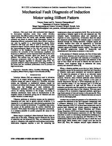
Fig. 2.18 - One slip cycle of the three phase stator current envelope for a threephase, 460V, 60-Hz, 6-pole, 5-hp squirrel-cage induction motor with four broken bars under rated load.

On the other hand, inter-turn short-circuits cause a profile modification of the three phase stator current leading to an envelope cyclically repeated at a rate equal to the power frequency (f). Moreover, an inter-turn short-circuit mainly affects the stator current


46

of the faulty phase in both profile and peak value. The other stator currents of the healthy phases are affected to a lesser degree. Thus, the stator current profile of each phase is not equally effected by the fault. This three phase stator profile modulation is referred to here as the envelope. Again, the frequency of repetition of this envelope is the power frequency, f. It is not a function of the slip frequency, spuf, which is associated with broken bar faults. The resulting envelope of the three phase stator currents for the same 5hp induction motor with four inter-turn short-circuits, without broken bars, experimentally obtained under rated load is shown in Fig. 2.19.

Fig. 2.19 - Three phase stator current envelope for a three-phase, 460V, 60-Hz, 6pole, 5-hp squirrel-cage induction motor with four inter-turn short circuits under rated load.


47

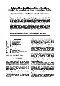
2.4.2 The air gap torque profile The air gap torque profile of an induction motor with broken bars is modulated proportionally to the three-phase stator current. The three-phase current envelope produces oscillations in the torque profile of an induction motor with broken bars that is cyclically repeated at the same rate 2spuf of the envelope in faulty motors. Such a relationship between the three-phase stator currents and torque can be seen in (2.26), in which the air gap torque is dependent of the three-phase stator current. The air gap torque profile for the same case-study induction motor of Fig. 2.18 under the same operating conditions is shown in Fig. 2.20. It is important to observe the same envelope characteristic in both signals, i.e. the frequency of the envelope and the oscillations of air gap torque are the same. The amplitude of the envelope and of the air gap torque is proportional to the motor load. If the motor is loaded, the amplitude of the envelope and of the air gap torque increases. Thus, the profile modulations of the envelope and torque are more evident. For the no load case, the amplitude of the envelope and the torque oscillations are very low. The frequency of the air gap torque oscillations for an induction motor with broken bars is twice the slip frequency [50]. Thus, the period of these oscillations Ttorque is given by (2.28) and is shown in Fig. 2.20.

Ttorque =

1 2 s pu f

,

(2.28)


48

where f is the power supply and spu is the per unit slip. Accordingly, the frequency of the air gap torque oscillations for faulty motors is load dependent. Thus, if the motor is loaded, the asynchronous speed (rotor speed) decreases, the slip increases, and the period of the torque oscillations increases.

35 30

Torque (Nm)

25 20 15 10 5 0

0

0.2

0.4

0.6

0.8 1 Time (s)

1.2

1.4

1.6

Fig. 2.20 – Air gap torque profile for a three-phase, 460V, 60-Hz, 6-pole, 5-hp squirrel-cage induction motor with four broken bars under rated load, at 1165r/min.

In conclusion, a review of basic concepts about induction motors and ac drives, as well as two types of induction motor faults, namely broken rotor bars and inter-turn short circuits in stator windings has been presented. Moreover, the physical phenomenon


49

associated with each of these faults was described, and two features of the induction motor performance resulting from these faults were presented. The feature used in the motor fault diagnostic method is the three-phase stator current envelope, while the feature used in the motor fault monitoring method is the air gap torque profile. The next chapter presents two methods to obtain the rotor speed and the air gap torque profile from the stator current and voltage signals, which are part of the monitoring method. Additionally, the machine learning techniques, which are used in both the monitoring and diagnostic methods, are presented in the next chapter.

Chapter 3: Induction Motor Features and AI Techniques

Chapter 3

50

Induction Motor Features and AI Techniques

CHAPTER 3 Speed and Torque Observers and Machine Learning Techniques This chapter describes the procedures to implement an air gap torque observer and a rotor speed observer. Both observers are used in the monitoring method. Moreover, an overview of the machine learning techniques used in both the diagnostic method and the monitoring method are presented in this chapter. Observers are used to substitute real sensors in several applications, such as vector control of ac drives and motor fault classification methods. Vector control of ac drives frequently requires speed or position sensors, while motor fault classification methods may require torque, speed, vibration, flux linkage, or temperature sensors. However, the use of physical sensors in these applications has some disadvantages, which include extra installation and maintenance costs, reliability problems, physical


51

limitations, and sensor cost. An alternative to this problem is to substitute these sensors by observers that mathematically estimate unknown variables from known variables. Thus, speed and torque observers for a motor-drive system can estimate speed and torque, respectively, from the available stator current and voltage signals. A torque observer and a rotor speed observer are discussed in the next two sections.

3.1

The Air Gap Torque Observer A torque observer estimates the torque profile of an induction motor from stator

currents and voltages. This estimation can be performed online in the order of milliseconds. Thus, a torque meter can be substituted by a torque observer even in applications that require fast torque measurements. Torque is usually calculated in the literature using several induction motor parameters that are not easily obtained [39, 43]. These parameters include the mutual inductances between rotor and stator windings, the inertia of the rotor, the rotor speed, and the rotor angular displacement. However, a torque observer can be based only on the stator voltages and currents of an induction motor [19, 51-55]. The stator currents and voltages are signals usually available, especially in motor-drive applications. The main equation for an air gap torque observer based exclusively on the stator voltages and currents is derived next. The air gap torque of a three-phase induction motor is given by [51, 54]:

T=

p

⎡ia (ψ c −ψ b ) + ib (ψ a −ψ c ) + ic (ψ b −ψ a ) ⎤⎦ , 2 3⎣

(3.1)


52

where p is the number of poles, ia, ib, and ic are the three-phase stator currents, and ψa, ψb, and ψc are the flux linkage of windings a, b, and c, respectively. See Appendix A for further details on the torque in (3.1). Algebraic manipulations in (3.1) yield (3.2).

p

⎡⎣ia (ψ c −ψ b −ψ a + ψ a ) + ib (ψ a −ψ c ) + ic (ψ b −ψ a ) ⎤⎦ 2 3 p ⎡ia (ψ c −ψ a ) + ia (ψ a −ψ b ) − ib (ψ c −ψ a ) − ic (ψ a −ψ b )⎤⎦ . T= 2 3⎣ T=

Hence, one can write the following:

T=

p 2 3

[iaψ ca + iaψ ab − ibψ ca − icψ ab ] ,

where:

ψ ca = ψ c −ψ a ψ ab = ψ a −ψ b .

Hence,

T=

p

⎡ψ ca ( ia − ib ) −ψ ab ( ic − ia ) ⎤⎦ . 2 3⎣

(3.2)


53

Substituting the flux linkages of the phases c and a given by (2.21) and the flux linkages of the phases a and b given by (2.19) into (3.2), the air gap torque is expressed as given in (2.26) and repeated in (3.3) for convenience as follows:

T=

p 2 3

{(ia − ib ) ∫ ⎡⎣vca − R (ic − ia )⎤⎦ dt − (ic − ia ) ∫ ⎡⎣vab − R (ia − ib )⎤⎦ dt} ,

(3.3)

where R is half of the line-to-line resistance, i.e. the phase resistance. Equation (3.3) is valid for Y-connected induction motor. However, for a delta connected induction motor, R must be divided by three [19]. Additionally, from (2.2) the phase current ib can be rewritten as

ib = − ( ia + ic ) .

(3.4)

Substituting (3.4) into (3.3), the equation of the air gap torque is expressed as (3.5), in which only two voltage sensors and two current sensor are required to calculate torque.

T=

p 2 3

{( 2ia + ic ) ∫ ⎡⎣vca − R (ic − ia )⎤⎦ dt − (ic − ia ) ∫ ⎡⎣vab − R ( 2ia + ic )⎤⎦ dt}.

(3.5)

This expression for torque can be easily computed in MATLAB® [56]. However, the integral can yield some difficulty. Thus, two considerations can be made. First, any dc


54

component in the voltages, currents, and flux linkages must be eliminated while the torque is being computed. Second, the integral can be computed by numerical integration using trapezoidal rule [57]. However, other methods such as rectangle rule and Simpson’s rule can also be used [57]. The main key is to calculate the torque for each period of the stator phase current, instead of for each single data point or for larger (more than one period of current) amount of data. The pseudo-code of the air gap torque observer is shown in Fig. 3.1.

1. Eliminate dc offset of vca, vab, ia, and ic. 2. Calculate ψca and ψab, using trapezoidal rule. 3. Build two vector ψ ca and ψ ab with the area calculated for each data point 4. Calculate the number of data points k for one period of ia. 5. Sum the k points of ψ ca and ψ ab , respectively. 6. Calculate the air gap torque by (3.5).

Fig. 3.1 – Pseudo-code of the air gap torque observer.

The air gap torque of a three-phase, 460V, 60-Hz, 2-poles, 2-hp squirrel-cage induction motor with five broken bars simulated using a finite element method (from a commercial software MAGSOFT) is shown in Fig. 3.2. This torque signal is directly obtained from the simulation. For comparison purposes, the three-phase stator currents and voltages obtained from the simulation of the above mentioned 2-hp induction motor


55

were used to calculate the air gap torque using the air gap torque observer. The torque signal calculated from the torque observer is shown in Fig. 3.3. The difference (error) between the signals of the Fig. 3.2 and Fig. 3.3 is shown in Fig. 3.4. The mean value of this error is 0.0443Nm, while the mean value of the torque simulated by FE method is 4.37Nm and the mean value of the estimated torque calculated by the air gap torque is 4.32Nm. Meanwhile, the mean square error between the torque simulated by FE method and the torque estimated by the torque observer is 0.0343Nm2 and the respective root mean square error is 0.1852Nm. Additionally, the per unit error, epu, can be calculated as follows:

e pu =

T − Tl , T

(3.6)

where T is the air gap torque simulated by FE methods, and Tl is the air gap torque estimated by the torque observer. The resulting per unit error, epu, of the signals shown in Fig. 3.2 and Fig. 3.3 is 1.01%, which demonstrates that both signals (T and Tl ) are very close. This experiment validates the efficacy of this air gap torque observer for fault monitoring purposes.


56

6

5

Torque (Nm)

4

3

2

1

0

1

1.5

2 Time (s)

2.5

3

Fig. 3.2 – Air gap torque profile for a three-phase, 460V, 60-Hz, 2-pole, 2-hp squirrel-cage induction motor with five broken bars under rated load simulated by finite element method. 6

5

Torque (Nm)

4

3

2

1

0

1

1.5

2 Time (s)

2.5

3

Fig. 3.3 - Air gap torque profile for a three-phase, 460V, 60-Hz, 2-pole, 2-hp squirrel-cage induction motor with five broken bars under rated load calculated by the air gap torque observer using the three-phase stator currents and voltages obtained from the simulation.


57

6 5

Torque (Nm)

4 Air gap torque from finite element simulations

3

Air gap torque from the torque observer

2 Error

1 0 -1

1

1.5

2 Time (s)

2.5

3

Fig. 3.4 – Error between the air gap torque obtained from finite element simulations and the air gap torque calculated by the torque observer using the three-phase stator and currents obtained from the simulations.

3.2

The Speed Observer Speed observers typically estimate the rotor speed of an induction motor from

easily acquired data, such as the three-phase stator voltages and currents. There are several methods to estimate rotor speed [39]. These methods can be divided into two groups, namely: (1) methods based on motor mathematical models, and (2) methods based on power spectral density. The methods based on motor mathematical models are the following: •

Slip calculation [39, 58]

•

Direct synthesis from state equations [39]

•

Model referencing adaptive system (MRAS) [39, 59]


58

•

Speed adaptive flux observer [39, 59]

•

Extended Kalman filter (EKF) [39, 60]

While the methods based on power spectral density are: •

Rotor Slot Harmonics (RSH) [61-63]

•

Injection of auxiliary signal [39, 64]

The speed observer used in the monitoring method in this thesis is based on rotor slot harmonics (RSH) because this method is easily implemented and is relatively accurated. Additionally, it does not require motor parameters and motor mathematical models. Moreover, this RSH-based speed observer is insensitive to motor parameter changes with frequency, temperature, or any other external disturbance. This speed observer uses the fast Fourier transform (FFT) [65] of only one phase stator current to detect the rotor speed at any load condition and over a wide range of speeds. Many improvements of speed observers based on rotor slot harmonic have been proposed in the literature [61-63, 66-69]. The principle of a rotor slot harmonics is discussed next. The rotor slots (or bars) produce a variation in the air gap permeance even if the slip, s, of an induction motor is zero. Air gap permeance is a measurement of the capability of the air gap to facilitate or impede the passage of magnetic flux. For clarification, the product of the air gap mmf and the air gap permeance, Pag, [63] produces the air gap flux and flux density, Bag. Thus, the air gap permeance interacts with the B

fundamental component of the air gap mmf to yield Bag. However, if the motor is loaded B

implying a slip greater than zero (s > 0), squirrel-cage bar currents circulate in the rotor


59

slots resulting in the rotor slot harmonics (RSH) which will also interact with Bag, which B

will be modulated at the rotor slot harmonic frequency fsh (in Hz) given in (3.7) [61-63].

f sh =

Z f r ± f0 , p

(3.7)

where Z is the number of rotor bars, p is the number of pole pairs, and fr = sf0 is the rotor frequency in Hz, where f0 is the power frequency supply also in Hz. It can be seen from (3.7) that fsh is only a function of the rotor speed, while the other terms are constants. Then, Bag induces an electro-motive force (emf) in the stator winding in such a manner B

that the rotor slot harmonics are reflected in the stator currents. Thus, a power spectrum analysis of the stator currents can be used to identify the RSH in order to obtain the rotor speed. With the rotor slot harmonic principle stated, the method to detect the rotor speed of an induction motor using a speed observer based on rotor slot harmonic analysis can be presented. The speed identification process is based on analysis of the FFT of only one phase stator current. Thus, the first step is to compute the FFT of any one of the three phase stator currents. The first search in the power spectrum of the phase current identifies the power frequency supply f0, which is the frequency component with the highest energy. The second step determines a window in the power spectrum to search for the RSH. This maximum frequency of the searching window fsh0 is given in (3.8).


60

⎛Z ⎞ f sh 0 = ⎜ − α ⎟ f0 , ⎝p ⎠

(3.8)

where α is order of the air gap flux density harmonic that can be 1 or -3 [61-63]. The width of the window Δfsh is given in (3.9).

Δf sh = Δf sh

Z sf o p

⎛ nsyn − nRATED =⎜ ⎜ nsyn ⎝

⎞Z ⎟ f0 , ⎟p ⎠

(3.9)

where s is the slip, nsys is the synchronous speed, and nRATED is the rated asynchronous speed, which is found on the nameplate of an induction motor. Thus, the window is defined in the interval [(fsh0 - Δfsh), fsh0]. This window is important to limit the search for the RSH to a small range of the power spectrum in order to minimize errors and improve computational performance. The third step is the search for the rotor slot harmonic fsh in the aforementioned window. The rotor slot harmonic is the frequency with the highest energy that is not an integer multiple of the power frequency f0. The last step is to calculate the rotor speed fr in Hz and the rotor speed n in r/min. There are two methods to calculate the rotor speed. The first method is used for induction motors in which the ratio Z/p is an integer. In this case, fr is calculated as follows:

fr =

p ( f sh + α f0 ) . Z

(3.10)


61

The relation between the rotor frequency, fr, and n is given by:

n=

60 fr . p

(3.11)

Thus, substituting (3.10) into (3.11) yields the rotor speed, n, as follows:

n=

60 ⎡ p ( f sh + α f0 )⎤⎥ ⎢ p ⎣Z ⎦

60 ( f sh + α f0 ) . Z

n=

(3.12)

The second method for computing n is used for induction motors in which the ratio Z/p is not necessarily an integer. Initially, this method estimate the slip frequency,

Δfr, as given by (3.13) assuming α=1:

Δf r =

p ( f sh0 − α f sh ) . Z

(3.13)

60 Δf r , p

(3.14)

Considering that,

Δn =


62

the slip speed, Δn, in r/min can be obtained by substituting (3.13) into (3.14). Thus, Δn is obtained as follows: Δn =

60 ⎡ p ( f sh0 − α f sh )⎤⎥ ⎢ p ⎣Z ⎦

Δn =

60 ( f sh0 − α f sh ) . Z

(3.15)

Thus, the rotor speed, n, can be calculated as follows: n = nsyn − Δn.

(3.16)

This method is now illustrated for a three-phase, 2-hp, 2-pole, 36 rotor bars, squirrel cage induction motor, operating at 80% of rated torque. The nameplate rated speed, nRATED, is 3450 r/min. The power spectrum of the stator current is shown in Fig. 3.5. The frequency with the highest energy (highest peak in the graph) is the power frequency f0 that was identified at 59.96Hz. The maximum frequency of the searching window fsh0 is thus calculated as follows:

⎛Z ⎞ f sh 0 = ⎜ − α ⎟ f 0 ⎝p ⎠ ⎛ 36 ⎞ f sh 0 = ⎜ − 1⎟ 59.96 ⎝ 1 ⎠ f sh 0 = 2098.6 2100 Hz.

(3.17)


63

0

59.96Hz

Power/frequency (dB/Hz)

-20

-40

-60

-80

-100

-120

-140

0

0.5

1

1.5

2

2.5

Frequency (kHz)

Fig. 3.5 – Power spectrum of the stator current of a three-phase, 2-hp, 2-pole, squirrel cage induction motor running at 80% of rated torque.

The width of the window, Δfsh, is thus calculated using (3.9) as follows:

⎛ 3600 − 3450 ⎞ 36 Δf sh = ⎜ ⎟ 59.96 3600 ⎝ ⎠ 1 Δf sh = 89.94 90 Hz.

(3.18)

Accordingly, the window [(fsh0 - Δfsh), fsh0] is [2010Hz, 2100Hz]. This power spectrum of the stator phase current restricted to this window is shown in Fig. 3.6. The frequency with the maximum energy, which is not an integer multiple of the power frequency, f0, was found at 2047.3Hz.


64

-70

2047.3Hz -75

Power/frequency (dB/Hz)

-80 -85 -90 -95 -100 -105 -110 -115 -120 2.01

2.02

2.03

2.04

2.05

2.06

2.07

2.08

2.09

2.1

Frequency (kHz)

Fig. 3.6 – Power spectrum of the window [2010Hz, 2100Hz] for the stator current of a three-phase, 2-hp, 2-pole, squirrel cage induction motor running at 80% of rated torque.

The ratio Z/p for this motor with Z = 2 and p = 2 is an integer. Thus, the rotor speed can be calculated using the two methods mentioned above. The first approach using (3.12) gives the result shown in (3.19).

n=

60 ( f sh + α f0 ) Z

60 n = ( 2047.3 + 59.96 ) = 3512.1rpm. 36

The second approach using (3.15) and (3.16) yields the following results:

(3.19)


Δn = Δn =

65

60 ( f sh0 − α f sh ) Z

60 ( 2100 − 2047.3) = 87.8rpm 36 n = nsyn − Δn

n = 3600 − 87.8 = 3512.2rpm.

(3.20)

Accordingly, both approaches yielded almost identical results. Meanwhile, the measured rotor speed for the induction motor of this example operating in the aforementioned condition was 3513 r/min. This test was repeated for different motor loads and the results are shown in Table 3.1. This table compares the measured speed and the estimated speed with the speed observer based on RSH. Moreover, the error between these two speeds was computed.

Table 3.1 – Speed estimated by a speed observer for a 2-hp, 2-pole, induction motor.

Torque 50% 80% 87% 93% 100%

2hp – 2poles – 60Hz – 36 rotor bars – Sine Excitation Measured speed Estimated speed 3545 3533.2 3513 3512.2 3505 3504.7 3500 3498.8 3494 3500.6

Error (%) 0.33 0.02 0.008 0.03 0.2

The next two sections discuss the machine learning techniques used in the diagnostic and monitoring methods. These techniques are called reconstructed phase space (RPS) and Gaussian mixture models (GMM).


3.3

66

The Reconstructed Phase Space The signatures of the diagnostic and monitoring methods in this thesis are

Gaussian mixture models obtained from the phase space reconstruction of the signals under investigation. These signals are digitized in order to generate a time series, which is expressed as follows [34]:

x = xn ,

n = 1...N ,

(3.21)

where, x, is the time series and xn is the instantaneous value of the signal for each sampled data point, n. Each data point is recorded at a rate given by the sampling frequency, fs, which results in a constant interval of time between two consecutive data points called the time sampling, τs. The sampling frequency fs is expressed as follows:

fs =

1

τs

.

(3.22)

The frequency, fs, must be at least twice the highest frequency of the signal in order to avoid aliasing distortions [65]. This factor is called the Nyquist rate. Here, Fig. 3.7 shows the phase (a) stator current, ia, of a 5-hp induction motor. This signal was sampled at 1kHz, which corresponds to a time sampling of 1ms. Therefore, this sampling frequency yielded 1000 data points per second, i.e. one data point per millisecond. Each data point is represented in Fig. 3.7 as a dot. Higher


67

frequency sampling yields a higher number of data points and higher signal resolution. However, the computational requirements to analyze this signal will increase with higher signal resolution. Thus, the sampling frequency selection should be based on the required resolution of the signal and the desired computational accuracy/performance. Again, the resolution of the signal is associated with the Nyquist rate, i.e. fs must be greater than twice the highest frequency of the signal. The sampling frequency of the signal shown in Fig. 3.7 is 1000Hz and the frequency of the fundamental component of this signal is 60Hz. Thus, fs is greater than twice the frequency of the signal, and accordingly aliasing distortion is not expected.

10

Current (A)

5

0

-5

-10

1

1.02

1.04 1.06 Time (s)

1.08

Fig. 3.7 – Stator current sampled at 1kHz.

1.1


68

The time series are used to reconstruct the phase space of a signal. A reconstructed phase space (RPS) is a technique used to observe the dynamics of a signal xn in a dimension greater that one. For instance, the one-dimensional representation of a signal is that obtained from a data acquisition system. The RPS projects the dynamics of an acquired signal in different coordinates. The number of coordinates to correctly reconstruct the phase space of the signal is the dimension, d [34, 35]. Specifically, instead of analyzing the dynamics of a signal in the conventional one-dimensional coordinate system, the dynamics of this signal can be reconstructed in a higher dimensional order d, where each coordinate is delayed in time, τ, from the present observation xn [35]. This time τ is called the time lag. Thus, the new coordinates of the RPS are composed by the present signal xn and by early observations of the system, such as xn-τ and xn-2τ. Accordingly, an RPS is defined as follows:

⎡ x1+( d −1)τ ⎤ ⎡ x1+( d −1)τ ⎢ ⎥ ⎢ ⎢ x 2+( d −1)τ ⎥ ⎢ x2+( d −1)τ X=⎢ ⎥=⎢ # # ⎢ ⎥ ⎢ ⎢ ⎢ x ⎥ N ⎣ ⎦ ⎣⎢ xN

x1+( d − 2 )τ

"

x1+τ

x2+( d −2 )τ

"

x2+τ

#

%

#

xN −τ

" xN −( d − 2 )τ

⎤ ⎥ x2 ⎥ , (3.23) ⎥ # ⎥ xN −( d −1)τ ⎥⎥ ⎦ ( N −( d −1)τ )×d x1

where N is the number of data points of the signal, d is the dimension, and τ is the time lag. The time lag is calculated by the automutual information function, I(τ), which is given as follows [35, 70]:


I (τ ) =

∑

xn , xn +τ

⎛ P ( xn , xn+τ ) ⎞ , P ( xn , xn+τ ) ln ⎜ ⎜ P ( x ) P ( x ) ⎟⎟ n n + τ ⎝ ⎠

69

(3.24)

where P(xn,xn+τ) is the joint probability density for the for the signal xn and xn+τ, which is delayed from xn by a time lag, τ, P(xn) and is the individual probability density for the signal xn, at the instant, n, and P(xn+τ) is the individual probability density for the signal xn+τ, at the instant, n+τ. Thus, xn and xn+τ are the same signal delayed from each other by a time lag, τ. If xn is independent of the xn+τ, then P(xn, xn+τ) becomes P(xn)P(xn+τ), and the automutual information is zero. The time lag, τ, that results in the first minimum of the automutual information, is chosen as the time delay to reconstruct the phase space of the signal, xn. The automutual information function is optimal for a dimension of two. Methods for calculating τ for higher dimensions are not currently known, thus, the time lag, τ, is calculated before the dimension, d. In the diagnostic and monitoring methods, the time lag is chosen when the first minimum of the automutual information is achieved. The behavior of the automutual information function can be shown through the next example. The signal of Fig. 3.8 is the normalized stator phase current of a 5-hp induction motor. The automutual information method was applied to this signal and the results are shown in Fig. 3.9. From this figure, the first minimum of this vector, which defines the time lag was found to be five.


70

2

Normalized current (A)

1.5 1 0.5 0 -0.5 -1 -1.5 -2

1

1.1

1.2

1.3

1.4

1.5

Time (s)

Fig. 3.8 – Normalized stator phase current of the 460-V,6-pole, 5-hp induction motor with four broken bars. 3.5

Automutual information

3

2.5

2

1.5

1

0

5

10

15

20 25 Time lag

30

35

40

Fig. 3.9 – Automutual information of the stator phase current for the 460-V, 6-pole, 5-hp induction motor with four broken bars.


71

On the other hand, the dimension d is calculated through the false nearest neighborhood (FNN) technique [34, 35, 70, 71]. When an RPS is built with low dimension, some neighbor points in the RPS are due to the projection of these points in the RPS, instead of the dynamics of the system. Accordingly, the false nearest neighborhood technique increases gradually the dimension of the RPS until all the points of the signal are unfolded, i.e. the RPS is free of false nearest neighbor points. Further increasing the dimension does not provide improvements for the representation of the dynamics of the signal through an RPS. Thus, an RPS might be generated with the lowest dimension that completely unfolds the signal. The false nearest neighborhood technique defines the dimension as follows. First, the square distance , Dn(d)2, between two points of the signal is computed as follows [70]: Dn ( d ) = x n ( d ) − x nNN ( d ) 2

Dn ( d )

2

d −1

2

(3.25)

2

⎤ = ∑ ⎡ xn−iτ ( d ) − x nNN −iτ ( d ) ⎦ , ⎣ i =0

where xn(d) is a point is an RPS with dimension, d, and time lag, τ, and xnNN(d) is nearest neighbor point to xn(d). The square distance that represents how far two neighbor points have moved from each other is given as follows [70]:

2

2 2 ⎤ Dn ( d + 1) − Dn ( d ) = ⎡ xn−dτ ( d ) − xnNN − dτ ( d ) ⎦ . ⎣

(3.26)


72

This square distance, Dn(d+1)2-Dn(d)2, is normalized as follows [70]:

2

Dn ( d + 1) − Dn ( d ) Dn ( d )

2

> Threshold rT ,

(3.27)

and the ratio, rT, results, which is compared with a threshold to define if a given point of an RPS is a false neighbor. Additionally, the percentage of false nearest neighbors is given as follows [70]:

⎛ 1 ⎜⎜ ⎝ N − ( d − 1)τ

⎛ D ( d + 1)2 − D ( d )2 ⎞ N n ⎞ ⎜ n ⎟ − rT ⎟, ⎟⎟ ∑ sgn ⎜ Dn ( d ) ⎠ n=1+( d −1)τ ⎜ ⎟ ⎝ ⎠

(3.28)

where N is the number of data points of the signal. This percentage is further compared to another threshold, which typically assumes values between 0.001 to 0.01. This comparison yields the appropriated dimension of the RPS that represents the dynamics of the signal under investigation. Again, the behavior of the false nearest neighborhood technique is demonstrated through an example based on the same signal of Fig. 3.8. The false nearest neighborhood for the signal of Fig. 3.8 was plotted in Fig. 3.10. The dimension is identified as the first dimension with the lowest percentage of false nearest neighbors. Thus, from Fig. 3.10 the dimension is identified as three. Higher dimension can be chosen, but this will not necessarily reconstruct the phase space with a better representation of the dynamics of the system.


73

Percentage of false neares neighbors

90 80 70 60 50 40 30 20 10 0

1

2

3

4

5 6 Dimension

7

8

9

10

Fig. 3.10 – False nearest neighborhood of the of the stator phase current for the 5-hp induction motor with four broken bars.

Thus, a RPS is completely defined in terms of the time lag and the dimension. For this example, the RPS has time lag five and dimension three. The RPS of the signal shown in Fig. 3.8 is presented in Fig. 3.11. Reconstructed phase spaces with a dimension higher than three can not be graphically represented. In such a case, the RPS is represented through a matrix such as in (3.23), where each column constitutes one of the dimensions of the RPS. For comparison purposes, the two-dimensional RPS of a perfect sine wave is an ellipse that can change in shape for different time lags.


74

1.5 1 x(n-2τ )

0.5 0 -0.5 -1 -1.5 1 1

0

0 -1

-1

x(n)

x(n-τ )

Fig. 3.11 – Reconstructed phase space of the phase stator current of the 5-hp induction motor with four broken bars.

The reconstructed phase space shown in Fig. 3.11, which has 1000 points (N=1000), dimension three (d=3), and time lag five (τ=5), is also mathematically expressed in (3.29).

⎡ x11 ⎤ ⎡ x11 ⎢ x ⎥ ⎢ x X = ⎢ 12 ⎥ = ⎢ 12 ⎢ # ⎥ ⎢ # ⎢ ⎥ ⎢ ⎣ x1000 ⎦ ⎣ x1000

x6 x7 # x995

x1 ⎤ x2 ⎥⎥ . # ⎥ ⎥ x990 ⎦ 990×3

(3.29)


75

Different signals yield different RPSs, and this can be observed in the RPS of the three-phase stator current envelope of a 2-hp induction motor with one broken bar shown in Fig. 3.12, and in the RPS of the air gap torque of a healthy 2-hp induction motor shown in Fig. 3.13.

3 2 x(n-2τ )

1 0 -1 -2 -3 2 1

2 1

0

0

-1 x(n)

-1 -2

-2

x(n-τ )

Fig. 3.12 – RPS of the three-phase envelope of the 460-V, 2-pole, 2-hp induction motor with one broken bar with τ = 5.


76

3

x(n-2τ )

1.5 0 -1.5 -3 3 1.5

3 1.5

0

0

-1.5 x(n)

-1.5 -3

-3

x(n-τ )

Fig. 3.13 - RPS of the air gap torque of the healthy 2-hp induction with τ = 20. Additionally, a RPS is frequency dependent, i.e. if the same signal is acquired with different sampling frequencies and the same time lag is used to build the RPS for both signals, the resulting RPSs are not the same. Thus, signal classification approaches based on RPS must deal with signals with the same sampling frequency in order to simplify this classification process using only one time lag.


3.4

77

The Gaussian Mixture Models A Gaussian Mixture Model (GMM) is an approach used for density estimation

[72]. A GMM with M mixtures is defined in (3.30) as follows:

M

p (x) =

∑ wm pm ( x ),

(3.30)

m=1

where M is the number of mixtures of a model, wm is the mixture weight [34] or mixing coefficients [72], pm(x) is the density function of the model. The constrains of mixture weight is given in (3.31) as follows:

M

∑ wm = 1,

(3.31)

m=1

where,

0 ≤ wm ≤ 1. Moreover, the probability density function of the model yields (3.32) as follows:

∞

∫−∞ pm ( x ) dx = 1.

(3.32)

For Gaussian mixture models, x is a Gaussian random variable with a probability density function, pm(x). The implementation of this density function can have several forms of the covariance matrix, Σm, such as spherical, diagonal, full, and PPCA


78

(probabilistic principal component analysis) [72]. The full covariance matrix is the form of the covariance matrix which is used in the diagnostic and monitoring method. The full covariance matrix can be any positive definite m×m matrix, Σm. A real matrix Σm is positive definite if the symmetric matrix, Σms is Σms=(1/2)( Σm +ΣmT) where

ΣmT is the transpose of Σm [57]. Moreover, the determinant of a positive definite matrix is positive, which implies that a positive definite matrix is nonsingular, i.e. it has an inverse. The density function of a full covariance matrix is given by (3.33) as follows [73]:

pm ( x ) =

1

( 2π )m 2 Σm 1 2

e

−

1 ( x − μm )T Σ−1( x− μm ) 2 ,

(3.33)

where μm is the mean value and Σm is the covariance of the Gaussian density function of each mixture M of the GMM. The covariance is the square of the standard deviation σ. Thus, pm(x) is a Gaussian density function represented by x~N(μm,Σm) with mean μm and covariance matrix Σm. A GMM with full covariance matrix is shown in Fig. 3.14. This figure shows the data points and three GMM parameters: centres, covariance axes, and one standard deviation error of each mixture.


4

79

Data points

3

Centres

2 1 0 -1 -2

One standard deviation error

-3 -4 -4

Covariance axis

-3

-2

-1

0

1

2

3

4

Fig. 3.14 – The full covariance matrix model.

The parameters of a GMM are estimated using an Expectation-Maximization

l , covariance Σ m , and mixture (EM) algorithm [34, 72, 74]. Thus, the estimated mean, μ m l m , are given in (3.34), (3.35), and (3.36), respectively as follows [34, 72]: weight, w

N

μl m =

∑ pm ( xn ) xn

n =1 N

∑ pm ( xn )

n =1

.

(3.34)


80

N

m = Σ

T ∑ pm ( xn )( xn − μm ) ( xn − μm )

n =1

.

N

(3.35)

∑ pm ( xn )

n =1

N

lm = w

∑ pm ( xn )

n =1 N M

.

(3.36)

∑ ∑ pm ( xn )

n =1 m =1

In the next chapter, the diagnostic and the monitoring methods are presented, in which the reconstructed phase space is used to build the Gaussian mixture model (signatures) for each class, i.e. for each motor operating condition. These GMMs are used to classify the induction motor faults in both methods, the diagnostic and monitoring method.

Chapter 4: Methodology

Chapter 4

81

Methodology

CHAPTER 4 Methods In this chapter, the induction motor fault diagnostic method and the induction motor fault monitoring method are presented. The diagnostic method classifies two different types of electrically detectable faults in induction motors: broken rotor bars and inter-turn short circuits in stator windings. Additionally, this method identifies the fault severity that is proportional to the number of broken bars or the number or percentage of short circuited turns computed by this method. This method is trained and tested with the datasets experimentally acquired from induction motors. The three-phase stator current envelope is the feature of the induction motors, which is used to build the fault signatures in order to classify the motor operating conditions. On the other hand, the monitoring method classifies the motor operating conditions of an induction motor as healthy or faulty, in which a faulty condition


82

represents any number of broken rotor bars. The monitoring method is trained with datasets generated using a commercial finite element software package (MAGSOFT) based on Finite Elements (FE) methods, and the monitoring method is tested with datasets experimentally acquired. The air gap torque profile is the feature of an induction motor used to build the signatures of the training and testing stages. This is a robust fault monitoring method because this algorithm is trained with only one dataset generated to a specific motor and it can monitor the fault of other induction motors independently of motor power, number of poles, motor load, and operating frequency. This monitoring method has the following two main advantages: •

The monitoring method is a robust technique to monitor induction motor faults, because this method is trained with datasets generated by FE simulations in order to monitor the operating condition of real motors. Thus, the training and monitoring stages of this method use datasets from different sources. The training stage uses datasets from FE simulations instead of datasets experimentally acquired, while the monitoring stage uses datasets from experimental setups. This characterizes the robustness of this method.

•

This monitoring method uses a novel normalization process. This normalization process is used to build fault signatures of the training and monitoring stages with similar amplitude and frequency. Thus, the signatures of the training and monitoring stages are independent of power, number of poles, level of load torque, and operating frequency, or other design characteristics of the motor being monitored. This is the case at least for the


83

two motors subject of this investigation. The monitoring method yields a relatively high degree of motor fault monitoring accuracy. Additionally, the monitoring method has also the following advantages: •

This monitoring method uses a small training set. The training set consists of two datasets (one for the healthy case and one for the faulty case) generated for only one induction motor simulated by FE methods, and this training set yields signatures that realistically represent the motor operating conditions of any other real induction motor, independent of power, number of poles, level of load torque, and operating frequency. This method yields a relatively high degree of motor fault monitoring accuracy, as will be demosntrated by the experimental results in Chapter 5.

•

This method is quickly trained because only two datasets (healthy and faulty) are needed in the training process instead of large datasets that include every single case related to different motor power, number of poles, motor load, and operating frequency. Accordingly, the small amount of training data needed in this presented method saves considerable time in generating the training set, since an FE simulation and experimentally acquired datasets require considerable time to obtain.

•

High costs associated with equipment to emulate the faults through destructive methods to generate datasets to train this method are not involved, since this AI-based method is trained with datasets generated by finite element (FE) methods, instead of datasets experimentally acquired.


•

84

This method uses only the three phase stator currents and voltages to build the signatures of the real motor and monitor its operating conditions. Thus, this method does not need complicated mathematical models of induction motors or values of motor parameters that are often difficult to obtain. Even the air gap torque (or developed torque) and the asynchronous speed (rotor speed) needed during the monitoring process are calculated through torque and speed estimators, respectively. These estimators only use experimentally acquired stator currents and voltages in addition to parameters that are commonly available from the nameplate data of motors.

Thus, this method constitutes a powerful tool for induction motor fault monitoring. Although, the diagnostic and monitoring methods use different procedures to obtain the training and testing sets, the training and testing stages of these methods are the same. The next section discusses the training and testing stages.

4.1

The Training and Testing Stages The diagnostic and the monitoring methods are based on machine learning

techniques [75], which consist of two stages: training and testing. The training stage uses the dataset called the training set to train the algorithm. The testing stage uses the dataset called the testing set to verify the classification accuracy of the algorithm. During the training stage, the diagnostic method uses datasets experimentally acquired, and the monitoring method uses datasets simulated by FE methods. However, both methods use datasets experimentally acquired in the testing stage.


85

The training set consists of different motor operating conditions, including faulty and healthy cases. Thus, from each motor operating condition, a signature is generated during the training stage of the diagnostic and monitoring methods. Additionally, the resulting trained algorithm is tested on the so-called “unseen signals”, which constitute the testing set. The accuracy of the motor fault classifier is defined in proportionality to the correctness of the classification of each faulty and healthy case to be identified in the testing set. The training signatures must properly represent the features of each motor operating condition to result in maximum fault diagnosis accuracy. The process of the training and testing stages is based on a previous work detailed in [34], in which one can also find the pseudo-code of the approach. The process consists of constructing a Gaussian Mixtures Model (GMM) [34] from a Reconstructed Phase Space (RPS) [34-36], where the resulting models are the signatures of the motor operating condition as outlined in the flowchart of Fig. 4.1. This RPS based approach allows for reconstruction of an induction machine’s state structure [71, 76]. The resulting fault signatures for the “unseen signals” are classified using a Bayesian maximum likelihood classifier [75]. This process has three steps as outlined in Fig. 4.1.


86

Training set

Testing set

Data Analysis

Normalization of the signals

Normalization of the signals

Time lag and dimension

Determine Time Lag

Construct the RPS for each sample of the testing set

Build GMM with M mixtures using EM

Determine Dimension Classification

GMM Models

Classify signals using Bayesian maximum likelihood classifier

Construct the RPS

Learn GMM with M mixtures using EM

Motor fault classification

Models, time lag and dimension

(a) Training stage

(b) Classification stage

Fig. 4.1 – The algorithm of the presented method. (a) Training stage. (b) Testing or classification stage.


87

The first step is data analysis in which the input signals from the training set are normalized to zero mean and are then scaled to unit standard deviation. Moreover, two parameters are calculated to construct the RPS: the time lag, τ,and the dimension, d. The time lag is calculated using the first minimum of the automutual information function, and the dimension is defined using the global false-nearest neighbor technique [34-36] as described earlier in Section 3.3. The second step is to learn a GMM of the RPS, i.e. the coordinates of the GMM are the d-dimensional RPS. The time lag and the dimension are used to build the RPS for each class of motor operating conditions. The GMM is learned with M mixtures for each class of motor operating conditions. The number of mixtures is related to the complexity of the models. A higher number of mixtures implies a more complex model. Ideally, a more complex model provides a higher accuracy in signals classification. However, in practice, there exists an optimal number of mixtures for maximum accuracy, and past that, the accuracy tends to be lower. Moreover, the parameters of the GMM, as centres and covariances, are estimated by an Expectation Maximization (EM) algorithm [34, 74] as described earlier in Section 3.4. A GMM of an RPS with dimension two (2), time lag nine (9) and eight (8) mixtures is shown in Fig. 4.2. Moreover, two parameters of the GMM, centres and covariances, are also shown in Fig. 4.2.


88

Fig. 4.2 – The Gaussian mixture model of the three phase stator current envelope of the 460-V, 6-pole, 5-hp faulty induction machine reconstructed phase space with eight (8) mixtures, dimension two (2) and time lag nine (9).

The last step is that of motor fault classification. The signature for an “unseen signal” is classified using the previously trained GMMs. The RPS of the “unseen signal” is constructed with the same dimension and time lag of the previously learned signatures. The Bayesian maximum likelihood classifier [75] computes the conditional likelihood of the signatures for this “unseen signal”, under each signature (Gaussian mixture model) previously learned using the training set as given in (4.1) below [34]:

p ( X | ci ) =

N

∏

n =1+( d −1)τ

p ( x n | ci ),

(4.1)


89

where X is the RPS matrix, d is the dimension of the RPS, τ is the time lag of the RPS, xn is a point in the RPS, N is the number of data points of the signal, and p(xn|ci) is the conditional probability of xn belonging to a class ci. The learned signature with maximum likelihood ĉ defines the particular class of motor operating condition (faulty or healthy) as given in (4.2) below [34]:

c = arg max p ( X | ci ) .

(4.2)

Again, the algorithm of this overall method is depicted in the functional flow chart of Fig. 4.1. In this figure, the results obtained in the training stage are followed by the fault classification in the testing stage. The training and testing stages discussed in this section are used in the diagnostic and monitoring methods to classify the faults of induction motors. The next section presents the diagnostic and monitoring method in association with the training and testing stages.

4.2

The Induction Motor Fault Diagnostic Method This section presents the induction motor fault diagnosis method and explains the

procedure used to obtain the three phase stator current envelope signals for broken rotor bars and inter-turn short-circuit fault cases.


90

The procedures used here to obtain the three phase stator current envelopes for broken bar and inter-turn short circuit cases for learning and classification are identical. This procedure can be summarized in the following steps: •

(1) Low pass filter (LPF)

•

(2) Envelope identification

•

(3) Interpolation

•

(4) Normalization

These steps are shown in the functional flowchart block diagram of Fig. 4.3. The first step is a low pass filter, which is essential for induction motors supplied by ac drives. The three-phase stator current of an induction motor supplied by an ac drive has high frequency components due to the carrier frequency responsible for the pulse width modulation (PWM) of the ac drive, as shown in Fig. 4.4a. Typically, the stator current frequency is variable from 0 to 60 Hz and the carrier frequency is a fixed value in the range from 4 to 16 kHz. Next, the ripple of the three-phase stator current is isolated as shown in Fig. 4.4b. This PWM component is eliminated from the ac current signal by a sixth-order lowpass elliptic digital filter with a cutoff frequency of 2 kHz, a passband of 3 dB, and a stopband of 50 dB [65]. Consequently, this results in the cleaner signal shown in Fig. 4.4c. The cutoff frequency was chosen to be 2 kHz because the carrier frequency of the ac drive is at least 4 kHz. Accordingly, the ripple is isolated from the three stator phase currents without any significant PWM component.


Fig. 4.3 - Algorithm of the induction motor diagnostic method. (a) Training stage. (b) Testing or classification stage

91

92

10

12

5

10

Current (A)

Current (A)


0 -5 -10 0

6

1000

2000 3000 Samples

4000

4 0

5000

1000

2000 3000 Samples

4000

5000

1000

2000 3000 Samples

4000

5000

1000

2000 3000 Samples

4000

5000

2 Normalized Current (A)

Normalized Current (A)

2 1 0 -1 -2 0

1000

2000 3000 Samples

4000

0 -1

2 Normalized Current (A)

1 0.5 0 -0.5 -1 -1.5 -2 0

1

-2 0

5000

1.5 Normalized Current (A)

8

1000

2000 3000 Samples

4000

5000

1 0 -1 -2 0

Fig. 4.4 – The process of obtaining the three-phase stator current envelope. (a) Three-phase stator current. (b) Ripple of the three-phase stator current. (c) Filtered ripple. (d) Envelope identification. (e) Interpolation of the envelope. (f) Normalization of the envelope.


93

The second step, which is the process of “envelope identification”, consists of extracting from the three phase currents only the positive peak of each period in each phase, as shown in Fig. 4.4d. The procedure to detect the peaks of the three-phase stator current consists of eliminating the dc-offset of the aforementioned ripple, detecting the zero-crossings, and finding the maximum value between two zero-crossings, which is the identification of each positive peak of each period in each phase. Thus, one second of a three-phase current signal at 60 Hz has 180 positive peaks. In the third step, these few points are interpolated to smoothly represent the dynamic behavior of the three phase stator current envelope, as shown in Fig. 4.4e. The fourth and last step is the z-score normalization that centers the signal at zero mean and scales it to unit standard deviation [77], as given in (4.3) below:

vnormalized =

v − μv

σv

,

(4.3)

where, μv is the mean value, and σv, is the standard deviation of the signal, v. A normalized three-phase stator current envelope is shown in Fig. 4.4f. Again, these steps which are used here to isolate the envelope of the three-phase stator currents of a given induction motor supplied by an ac drive can best be visualized by inspection of the functional block diagram flowchart of Fig. 4.3. After accomplishing these four steps, the identified envelope is used to generate the training set to learn the GMMs (signatures) that represent each type of fault, or to


94

generate the testing set in order to classify an unseen input signals by a maximum likelihood Bayes classifier [75], as discussed in the previous section. Thus, this method creates signatures for each type of fault based on the three phase stator current envelope. A signature for each newly acquired input set of three phase stator currents, which are called “unseen signals”, is generated and compared with all signatures that represent each type of fault learned from the previously acquired database. The conditional likelihoods among this new signature and the previously learned signatures for each type of fault are calculated. Thus, a maximum likelihood Bayes classifier identifies the previously learned signatures with a maximum likelihood, which now classifies the fault of the so-called “unseen signal” undergoing the process of classification. In this diagnostic method, the classification process yielded high accuracy using just a half second of current signal for a 3-phase, 460V, 60-Hz, 6-poles, 5-hp squirrel-cage induction motor, which is roughly the time equivalent to a third of a slip cycle under normal loads. This will be shown and supported by the experimental results presented later in the Chapter 5 of this thesis. Additionally, the diagnostic method utilizes only three current sensors, which are easily available and implementable in most industrial applications. In most drives this current information is readily available and hence no extra current sensors are needed to implement this diagnostic method.


4.3

95

The Induction Motor Fault Monitoring Method The monitoring method, which is not a specific fault identification/diagnostic

method, is used to classify the motor operating condition of an induction motor as either healthy or faulty. The high level algorithm of this method is shown in functional block diagram flowchart form in Fig. 4.5, while the detailed steps of algorithm are shown in the flowchart of Fig. 4.6.

Fig. 4.5 – The high level algorithm of the monitoring method.


96

nsyn =

120 f P

[ rpm]

nsFE = nsyn − nasy

TFE =

60 nsFE P

NpsFE =

[ rpm]

[ s]

1 TFE

nsyn = 120 f P

[ rpm]

nsRM = nsyn − nasy

TRM = 60 nsRM P TSlength = NpsFE × TRM

[ rpm]

[s] [ s]

Fig. 4.6 – Detailed algorithm for the induction motor fault monitoring method


97

The monitoring method is divided in two stages: the training stage and the monitoring (testing) stage. During the training stage, the monitoring method generates signatures (model) from healthy and faulty induction motor simulations in MAGSOFT (FE software). These signatures are generated from the air gap (developed) torque profile of each healthy and faulty operating condition obtained directly from the simulations. Here, the faulty condition is that of a motor with one broken rotor bar case at rated load and speed. The algorithm of the training stage has three steps. In the first step, datasets with two seconds of the air gap torque profile for faulty and healthy cases are obtained directly from MAGSOFT. Each dataset is divided into two time series of one second each. This yields two time series of one second each for the healthy case and two time series of one second each for the faulty case. The time series of the air gap torque for the one broken bar case with a duration of one second is shown in Fig. 4.7a. The dc offset of each time series is eliminated in order to avoid filtering errors, which results in the time series profile shown in Fig. 4.7b. Subsequently, the high frequency components of each time series are filtered by a sixth-order lowpass elliptic digital filter with a cutoff frequency of 100 Hz, a passband of 0.1 dB, and a stopband of 50 dB [65]. This results in the time series shown earlier in Fig. 4.7c. The second step is the data analysis, in which the torque signals are normalized by the formulation in (4.3). An example of the normalized air gap torque profile is shown in Fig. 4.7d. Moreover, two parameters are computed to build the Reconstructed Phase


98

Space of each motor operating condition: time lag (τ) and dimension (d), as described earlier in Section 3.3. The last step is to learn the signatures. The time lag and dimension, previously calculated, are used to build a Reconstructed Phase Space for each class, i.e. for the healthy and faulty cases. Thus, a Gaussian Mixture Model of each RPS is learned, and the resulting models are the signatures of the motor operating conditions.

Air gap torque (Nm)

1

4 3 2 1 0 0

500

1000 Samples

1500

Air gap torque (Nm)

1 0.5 0 -0.5 -1 0

500

1000 1500 Samples

2000

0.5 0 -0.5 -1 0

2000

Normalized air gap torque (Nm)

Air gap torque (Nm)

5

500

1000 1500 Samples

2000

1000 Samples

2000

3 2 1 0 -1 -2 -3 0

500

1500

Fig. 4.7 – The process of obtaining the air gap torque profile for the training stage of the monitoring method for the 2-hp induction motor at 60Hz and rated torque with one broken bar simulated by finite elements software. (a) Air gap torque from the MAGSOFT. (b) Torque without dc offset. (c) Filtered torque signal. (d) Filtered and normalized torque signal.


99

Simultaneously, the number of periods of oscillations of the air gap (developed) torque profile in one second, NpsFE, must be calculated. Then, three parameters can be obtained from MAGSOFT: frequency of the power supply f, number of poles P, and asynchronous (rotor) speed nasy. The synchronous speed, nsyn, is given in (2.9) and repeated below in (4.4) for convenience:

nsyn =

120 f . P

(4.4)

Moreover, the slip speed nsFE in r/min is computed as (2.10) and also repeated in (4.5) for convenience. nsFE = nsyn − nasy .

(4.5)

The period of each oscillation of the air gap torque profile TFE of a faulty case is related to the slip speed and number of poles as given below in (4.6). The parameter TFE is given in seconds. The parameter TFE is equivalent to TRM in Fig. 4.9.

TFE =

60 . nsFE P

(4.6)

Thus, NpsFE is accordingly given in (4.7) as follows:

NpsFE =

1 TFE

.

The parameter NpsFE is used during the testing stage.

(4.7)


100

On the other hand, the testing stage uses datasets experimentally acquired. The testing stage can be divided into the following steps described below. For the acquired voltage and current signals from real motors, the air gap torque is estimated using a torque observer as demonstrated in equation (3.5) of Section 3.1. An example of the resulting air gap torque signal from this torque observer for a 3-phase, 460-V, 60-Hz, 6-poles, 5-hp squirrel-cage induction motor at rated speed and load is shown in Fig. 4.8a. The torque signal is divided in time series of a period of one second, and subsequently the dc offset is eliminated from that signal as shown in Fig. 4.8b. Moreover, the resulting torque without the dc offset is filtered by the same low pass filter used during the training stage. The resulting filtered air gap torque signal without dc offset is shown in Fig. 4.8c. The synchronous speed, nsyn, and the slip speed, nsRM, for the testing set that uses data from a real motor (RM) are as given in (4.4) and (4.5), respectively, with the replacement of the subscript, FE, by the subscript, RM. Additionally, the period of each oscillation of the air gap torque profile, TRM, for a real motor is as given by (4.8) below. This TRM is 0.29s in Fig. 4.8a and b, i.e. the period of each cycle of the air gap torque in a faulty case is 0.29s. Thus, in one seconds there are 3.5 cycles (1/0.29s = 3.5Hz). The value of TRM associated with one slip cycle of a normalized air gap torque signal is depicted in Fig. 4.9, and can be expressed as follows:

TRM =

60 nsRM P

.

(4.8)


101

A speed rotor observer based on rotor slot harmonics (RSH) is used to estimate the asynchronous (rotor) speed, nasy, as was described earlier in Section 3.2.

Air gap torque (Nm)

32 30 28 26 24 0


5

500

1000 Samples

1500

2 1 0 -1 -2 -3 0

500

1000 Samples

1500

2000

2.5 0 -2.5 -5 0

2000


Air gap torque (Nm)

34

500

1000 1500 Samples

2000

1000 Samples

2000

2 1 0 -1 -2 -3 0

500

1500

Fig. 4.8 – The process of obtaining the air gap torque profile for the testing stage of the monitoring method for the 5-hp motor at rated speed and load torque. (a) Air gap torque obtained from a torque observer. (b) Air gap torque without dc offset. (c) Filtered air gap torque signal without dc offset. (c) Air gap torque profile after the frequency normalization process.


102

34 33 32 Torque (Nm)

31 30 29 28 27 26 25

0

0.2

0.4

0.6

0.8 1 Time (s)

1.2

1.4

1.6

Fig. 4.9 - Air gap torque profile of the 6-pole, 60Hz, 5-hp motor with 4 broken bars in which TRM is shown in one slip cycle. The length (or duration) in seconds of each time series TSlength is accordingly as given below in (4.9):

TSlength = NpsFE × TRM .

(4.9)


103

The duration, TSlength, is used in the frequency normalization process in order to digitally obtain TRM with the same number of data points (samples) as TFE. In other words, the duration, TSlength, is used to obtain each time series of the testing set which will have the same fundamental frequency component of the training set for healthy and faulty cases. For example, the air gap torque for a faulty case in the training set was found to contain 2.9 cycles in one second as previously shown in Fig. 4.7d, while the air gap torque for a faulty case in the testing set was found to contain 3.5 cycles in one second as shown in Fig. 4.8a. Clearly, both signals have different frequencies. However, the reconstructed phase space that is used to build the signatures of the motor operating condition is frequency dependent, i.e. if the signatures from the training and testing stages are not built with signals with the same frequency, susceptibility to misclassification increases. Accordingly, the duration, TSlength, was found to be 0.84s in Fig. 4.8c. This corresponds to 1688 samples (data points) in order to obtain a torque signal for the testing set with 2.9 cycles, which is the same length of the training set. Then, this air gap torque signal is truncated at 0.84s (2.9 cycles or 1688 data points). Thus, the signal at the instant of time greater than 0.84s up to 1s is discarded. Using upsampling and downsampling processes [65], the remaining air gap torque signal of the testing set can be rebuilt with the same frequency or number of samples as that of the testing set, thus yielding both signals (training and testing) with the same fundamental frequency component as shown in Fig. 4.8d. It is well-known that the period of each torque oscillation, TRM, is both load and operating frequency dependent, and consequently slip speed dependent. Accordingly, this resampling of the torque signals yields a motor fault monitoring method independent


104

of the level of load torque, operating frequency, power, and number of poles of an induction motor. The next step is to learn the signatures for each new torque signal. This signal is normalized and a new RPS is built with the same time lag (τ) and dimension (d) of the training stage. Then, a GMM is learned from this new RPS to obtain a signature for this new torque signal. The last step is the monitoring, in which the conditional likelihoods of this new signature obtained during the testing stage and the previously learned signatures generated during the training stage are computed. A Bayesian maximum likelihood classifier as given earlier in (4.1) and (4.2) is used to identify the signature of the training stage with the maximum likelihood. The class of this signature defines the motor operating condition: healthy or faulty. This chapter presented the diagnostic method and the monitoring method, which are next used to classify and monitor induction motor faults, respectively. In the next chapter, the experimental verification of these methods and a discussion of the results are presented.

Chapter 5: Experimental Verification of the Presented Method

Chapter 5

105

Experimental Verification of the Presented Method

CHAPTER 5 Experimental Verification of the Methods In this chapter, the experimental verification of the diagnostic and monitoring methods discussed in Chapter 4 is presented. The results given in this chapter validate these two methods used for classification and monitoring of induction motor faults. The results of each method are followed by a discussion of these results.

5.1 Results for the Induction Motor Fault Diagnostic Method A case-study 3-phase, 460-V, 60-Hz, 6-poles, 5-hp squirrel-cage induction motor supplied by an ac drive operating under scalar (open-loop) constant Volts per Hertz control was tested in the laboratory, as shown in Fig. 5.1.


106

Fig. 5.1 - Laboratory test setup for a 5-hp induction motor data acquisition. This motor has a cage with 45 bars, that is 7 ½ bars per pole pitch, and it has 240 stator winding turns per phase housed in a stator with 36 slots, that is six slots per pole, and hence two slots per pole per phase. This motor was tested under healthy and one through four broken bars of rotor faulty conditions, as well as one through four inter-turn shorts in one phase of the stator windings. Thus, this set of tests yielded nine classes of induction motor operating conditions. An external resistor, rf, of 1Ω was used to emulate a developing or an “incipient” inter-turn short-circuit in the stator windings as depicted in Fig. 5.2. This resistor also restricts the circulating currents in the shorted portion of the stator winding to a safe level to avoid permanent motor winding damage. In these tests,


107

the loop current in the shorted turn was not allowed to exceed in rms magnitude three times the rated line current of the motor.

Fig. 5.2 - The schematic of stator winding tappings for the tested induction motors. The three phase stator current was sampled for each class at a 50 kHz sampling frequency using the data acquisition board shown in the functional schematic of Fig. 4.3. Each class has five seconds of signal which results in 250,000 points each. These five seconds of signal were equally divided into 10 samples where each sample is a time series. Thus, the procedure depicted in Fig. 4.3 was carried out and the resulting totality of ten time series of each class yielded the training set as well as the testing set using a cross-validation technique [75, 78]. Cross-validation is a well-known technique used when the dataset is not large enough to obtain totally independent training and testing sets. The cross-validation splits the same dataset generating different training and testing


108

sets. The training and test sets were generated by k-fold cross-validation with k=10, see [75, 78]. The experiment carried out for broken bars has five classes (one through four broken bars and the healthy case), and for inter-turn short-circuits it has also five classes (one through four inter-turn short-circuits and the healthy case). However, the last experiment combines all faults plus the healthy case, thus resulting in nine classes. Accordingly, the number of samples of the testing set generated using k-fold cross-validation is defined by the number of time series per class times the number of classes. These samples of the testing set are distributed in k folds. Thus, an experiment with five classes, k=10, and ten time series per class has a testing set with 50 samples distributed in 10 folds that are to be classified. The motor current envelopes obtained from the experimentally acquired motor current data represent two types of motor faults: broken rotor bars and inter-turn shortcircuits in stator windings. The experiment for broken bars was carried out for three different motor loads, and for two different ac drive output frequencies yielding two different motor speeds. While the experiment for the inter-turn short-circuits in stator windings was carried out for three values of motor loads at one ac drive output frequency. Finally, the last experiment for broken bars and inter-turn short-circuits yielding nine classes of motor operating conditions was carried out for three levels of motor loads, also at one ac drive output frequency. All experimental results presented below validate the efficacy of this method.


109

The above mentioned case-study 5-hp three-phase, squirrel-cage induction motor, with one through four broken rotor bar faults was tested in the laboratory. The fault classification results for broken bars with the motor running at 60 Hz and three different levels of loads are shown in Table 5.1. The results for each combination of mixtures of the fault signatures and levels of load torque shown in Table 5.1 were generated using a testing set with 50 samples obtained by 10-folds cross-validation. Here, each sample has a duration of 0.5s of three phase stator current envelopes. Accordingly, the one through four broken rotor bars and the healthy motor case yield five classes of motor operating conditions. Again, the motor was tested with three different magnitudes of load which correspond to 50, 75 and 100% of the rated torque. It should be pointed out that the rated torque is 30Nm. As given in Table 5.1, the accuracy of the resulting fault classification for a motor load of 50% and 100% of the rated torque was 100%, i.e. all 50 unseen input samples of the testing set were correctly classified independent of the number of mixtures

Table 5.1 - Accuracy of fault classification for a 5-hp, 6-pole, induction motor with one through four broken bars at 60 Hz and three different motor loads based on a testing set with 50 samples. Accuracy (%) (mean ± standard deviation)

Mixtures 4 8 16 32

Motor load as % of Rated Torque 50% 75% 100% 100±0 100±0 100±0 100±0 98±6 100±0 100±0 100±0 100±0 100±0 100±0 100±0


110

of the fault signatures. The same level of accuracy was obtained for a motor load of 75% of the rated torque with four, 16 and 32 fault signature mixtures. However, a slightly lower fault classification accuracy of 98% was obtained and is shown in Table 5.1 for the 75% of the rated torque case with eight fault signatures mixtures, which means that only one of the 50 samples of the testing set was misclassified. Additionally, the presented fault classification method not only monitors the faults, thus distinguishing a faulty motor from a healthy motor, but also diagnoses the degree of fault severity identifying the number of broken bars. Here, the degree of fault severity is proportional to the number of broken bars. Furthermore, the presented results were carried out for motor loads over 50% of the rated torque. However, the accuracy of fault classification for motor loads below 50% of the rated torque is slightly lower compared to the accuracies obtained for motor loads above 50% of the rated torque. Below 50% of the rated torque, the amplitude and profile of the envelopes for any number of broken bars become very similar to the healthy case in which the amplitude of the envelope is ideally zero. Thus, when signals with similar envelopes are obtained for a given operating condition under healthy and faulty operations, the implication is that there will be difficulties building sets of signatures that represent efficiently the motor fault operating conditions for accurate motor fault classification. In general, this confirms the well-known fact that it is harder to diagnose a fault when a motor is lightly loaded [14, 29, 31]. This is an aspect which is further elucidated in the Section 5.2 of this chapter.


111

Here, Table 5.2 presents the accuracy of the broken bar fault classification for the 5-hp motor at rated torque and two different ac drive output frequencies of 40 Hz and 60 Hz, respectively. The results for 60 Hz are the same as previously shown in Table 5.1. The testing set for the results at 40 Hz contains 30 samples instead of 50 samples because the original 5s of current signals for each class had to be divided in six samples instead of 10 samples, thus yielding the three phase stator current envelope for each sample with a duration of 0.83s (5s / 6 time series per class). This higher time sample for the 40 Hz data compared to the 60 Hz data is necessary to have samples with approximately the same number of envelope periods for both cases. This time sample of each input signal which is to be classified can be associated with the operating motor frequency in order to automatically adjust the length of the time sample to be used in the classification, because the motor frequency and the length of the time sample are inversely proportional to each other. An accuracy of 97% was obtained and is shown in Table 5.2 at 40 Hz for four and eight fault signature mixtures, which means that this method resulted in only one

Table 5.2 - Accuracy of fault classification for a 5-hp, 6-pole, induction motor with one through four broken bars at 40 and 60 Hz based on a testing set with 30 samples. The test was carried out at rated load. Accuracy (%) (mean ± standard deviation)

Mixtures 4 8 16 32

Motor frequency 40 Hz 60 Hz 97±10 100±0 97±10 100±0 90±16 100±0 77±16 100±0


112

misclassification out of thirty. Table 5.2 includes results with 90% classification accuracy for 16 fault signature mixtures, which means that this method resulted in three misclassifications out of thirty. Meanwhile, an accuracy of 77% for 32 fault signature mixtures was achieved, which means that this method resulted in seven misclassifications for the testing set with 30 samples. The second type of motor fault investigated with the diagnostic method is the inter-turn short circuit. This type of motor fault has five classes: one through four interturn short-circuits and a healthy case. The accuracy results for classification of the interturn short-circuits in the 5-hp motor at 60 Hz and motor loads of 50, 75 and 100% of the rated torque are given in Table 5.3. The motor fault classification is highly accurate with a low standard deviation in all cases shown in this table. These results were based on a testing set with 50 samples. Thus, a 98% accuracy of classification was achieved, which represents only one misclassification out of fifty. Meanwhile, the case with 96% classification accuracy represents two misclassification and so forth. The different levels of load torque did not result in any loss of accuracy for classification of inter-turn shortcircuits. This lack of effect of load level on classification results of the shorted turn faults in comparison to the opposite for the cases with broken bars is physically explained in the next section. From Table 5.3, it can be concluded that signatures with 16 mixtures are sufficient for achievement of a reasonably high degree of accuracy. However, models with eight mixtures can speed up the learning and classification processes without significant losses in the fault classification accuracy. These fault classification results and associated method constitute a significant contribution for motor fault classification


113

techniques considering that inter-turn short-circuits represent 30 to 40% of the commonly occurring motor faults, with the knowledge that in this method at hand only envelopes of the three phase stator currents are needed. Table 5.3 - Accuracy of fault classification for a 5-hp, 6-pole, induction motor with one through four inter-turn short-circuits in the stator windings at frequency of 60 Hz and motor loads of 50, 75 and 100% of the rated torque based on a testing set with 50 samples. Accuracy (%) (mean ± standard deviation)

Mixtures 4 8 16 32


The last experiment was carried out for one through four broken bars, one through four inter-turn short circuits and the healthy motor case yielding nine classes of operating conditions. Thus, these nine classes yielded a testing set with 90 samples generated by a 10-folds cross-validation method. The accuracy results for classification of the nine different motor operating conditions for the above mentioned 5-hp motor at 60 Hz and motor loads of 50, 75, and 100% of the rated torque are given in Table 5.4. The data in this table also shows that a more accurate classification result was obtained for fault signatures with 32 mixtures for any level of motor load over 50% of the rated torque, in which case only one of the 90 samples of the testing set was misclassified, thus yielding a 99% classification accuracy. These results for 32 fault signature mixtures can be better


114

observed in the so called “confusion matrix” [78] given in Table 5.5. The confusion matrix reports the performance of a classifier. It is a square matrix with its dimension defined by the number of classes. The sum of components of each row must contain the same number of samples of the testing set. Each combination of row i and column j contain the number of samples of the testing set classified as the class of the respective column j. A confusion matrix that represents a perfect classifier is a diagonal matrix. Additionally, Table 5.5 demonstrates that only one fault was classified as a broken bar fault, when it should have been classified as an inter-turn short-circuit. For clarification, it should be pointed out that the headings for the confusion matrix of Table 5.5 are defined as follows: 1BB ≡ one broken bar, 2BB ≡ two broken bars, 3BB ≡ three broken bars, 4BB ≡ four broken bars, H ≡ healthy, ST1 ≡ one turn short circuited, ST2 ≡ two turns short-circuited, ST3 ≡ three turns short-circuited, and ST4 ≡ four turns short-circuited. These results demonstrate the relatively high degree of accuracy of fault classification associated with use of this diagnostic method.

Table 5.4 - Accuracy of fault classification for a 5-hp, 6-pole, induction motor with one through four broken bars or one through four inter-turn short-circuit in stator windings at frequency of 60 Hz and motor loads of 50, 75 and 100% of the rated torque based on a testing set with 90 samples. Accuracy (%) (mean ± standard deviation)

Mixtures 4 8 16 32



115

Real faults

Table 5.5 - Confusion matrix for the 99% classification accuracy of the 5-hp, 6-pole, induction motor with one through four broken bars or one through four inter-turn short-circuit in stator windings at frequency of 60 Hz and motor loads of 50, 75 and 100% of the rated torque based on a testing set of 90 samples and with 32 fault signature mixtures.

1BB 2BB 3BB 4BB H ST1 ST2 ST3 ST4

Classified faults 1BB 2BB 3BB 4BB H ST1 ST2 ST3 ST4 10 0 0 0 0 0 0 0 0 0 10 0 0 0 0 0 0 0 0 0 10 0 0 0 0 0 0 0 0 0 10 0 0 0 0 0 0 0 0 0 10 0 0 0 0 1 0 0 0 0 9 0 0 0 0 0 0 0 0 0 10 0 0 0 0 0 0 0 0 0 10 0 0 0 0 0 0 0 0 0 10

5.2 Discussion of Results for the Induction Motor Fault Diagnostic Method In this thesis, a 5-hp induction motor was investigated for monitoring and diagnosis of broken rotor bars and inter-turn short-circuits in stator windings under three different magnitudes of motor loads. The three phase stator current envelope was found here to be a powerful feature of the induction motor for fault classification. Each healthy and faulty motor operating condition yielded a signature generated from the three phase stator current envelope using Gaussian Mixture Models of Reconstructed Phase Spaces. The conditional probability of a fault signature for any “unseen signal” was computed for each given signature previously generated during the training stage. Thus, this “unseen signal” was classified using the Bayesian maximum likelihood classifier.


116

The three phase stator current envelope for broken bar faults depends on the number and geometric distribution of the broken bars. Two motors with identical ratings and with the same number of broken bars, but with different geometrical distributions of the broken rotor bars may yield a misclassification of this fault, because the signatures are learned for a specific number and distribution of broken bars. Different distributions for the same number of broken bars may yield different signatures. Thus, a signature learned for a specific number and distribution of broken bars can not guarantee a correct classification of the same number of broken bars for different geometrical distributions. This is an open problem not only for the method presented in this thesis, but also for other techniques which analyze the stator currents [7, 10]. The diagnostic method is based exclusively on the analysis of the three phase stator current envelopes. The inputs of the presented method are only the training and testing sets composed from experimentally obtained samples of three phase stator current envelopes for different motor operating conditions. Thus, there is no need for any other information about the induction motor or its various parameters during the training and testing stages. Moreover, mathematical models of the induction machines, or the ac drives, or any other mathematical formulation or knowledge about the induction motor are not required. This simplifies the motor fault classification problem because complex calculations related to induction motors as well as any specific design information about each individual motor for the purposes of fault diagnostics are not involved. However, the presented method at this point needs signatures built for each different fault at different speeds and torques. This yields many signatures to represent the range of all


117

possible motor operating conditions. Therefore, the number of signatures may be reduced if the signatures built for a specific operating condition, for example, rated speed and torque, are scaled for any other different operating condition. In this case, the signature generated for the rated conditions must be associated with speed and torque in order to scale it for use in any other motor operating condition. The speed can be obtained either directly from the ac drive, or from a speed sensor, or from a speed observer. The torque can be either measured by a torque transducer, or calculated through a torque observer. Thus, the signatures can be automatically redefined for any value of speed and torque of an induction motor. The presented method yielded a high degree of accuracy of motor fault classification even with the induction machine running at different levels of load torque. This statement is best validated by careful examination of Table 5.4, which presents the accuracies of fault classification for nine different healthy and faulty cases of the 5-hp induction machine. Moreover, Table 5.4 shows the accuracy of motor fault classification for three different levels of load torque and four different numbers of fault signature mixtures. Here, the number of mixtures is manually defined through the analysis of the classification results. From an investigation of Table 5.4, it can be concluded that 32 mixtures is the best number of fault signature mixtures because the accuracy remains high at 99% for any level of motor load. However, the speed of the training and testing stages of the presented method is directly related to the number of fault signature mixtures. Thus, the diagnostic method can be more efficiently computed by using fewer fault signature mixtures. From further examination of Table 5.4, it can be concluded that


118

accuracy over 97% was obtained with eight fault signatures mixtures for any level of motor load over 50% of the rated load, which is deemed reasonable for general industrial applications. In this case, eight mixtures satisfy the requirement for both a reasonable level of fault classification accuracy and required time of the training and testing processes. The well-known difficulties normally associated with diagnosing motor faults at light loads [14, 29, 31] were also encountered here. It is observed that the accuracy of this diagnostic method deteriorated for motor loads under 50% of the rated load values. This is not a new difficulty and other methods documented in the literature suffer from similar problems [14, 29, 31]. This can be physically attributed to the fact that under light load the rotor electric circuit approaches the high impedance associated with the no-load condition, in which the effect of any change in the cage impedance can be masked due to its weak impact at the stator terminals. Furthermore, from a magnetic field point of view, at rated or near rated load the currents in the bars of a squirrel cage act as a magnetic shield to the bulk of the rotor iron core, and hence that core remains relatively unsaturated or lightly saturated, with a good degree of magnetic circular symmetry (no magnetic saturation induced saliency effects). When bar breakages do occur at rated, or near rated, load conditions, the magnetic shielding effect of the bars is lost at the location of such a bar breakage, with a resulting higher degree of local magnetic saturation appearing at that spot. Hence, the rotor’s circular magnetic symmetry is lost and an “apparent magnetic saliency or asymmetry” appears in the rotor. This asymmetry rotates at slip speed with respect to the synchronously rotating magnetic field, and this


119

asymmetry gives rise to the envelope appearing to enclose the three-phase current waveforms. Hence, it is easier to diagnose such a fault using such an envelope under such substantial motor loads. This phenomenon which was exploited here is reduced at light loads, and hence gives rise to the difficulty in diagnosis below 50% of rated load for the 5-hp case-study motor. Although, a short circuit between turns of two phases and a short circuit in turns of all phases due to overload or blocked rotor are possible, an inter-turn short-circuit generally occurs first in just one phase. In this case, the stator current envelope of each single phase is not modulated equally. The stator current envelope of the healthy phases is slightly affected by the faulty phase, while the envelope of the faulty phase is highly modulated. Here, an analysis of the stator current envelope of only one phase instead of the three phases can not be sufficient to diagnose correctly a faulty condition, particularly if this analyzed phase is not the faulty phase. This addresses the reason for the use of a three phase stator current envelope instead of a single phase stator current envelope. Independent of the phase in which turns are short-circuited, the three phase stator current envelope associated with the method presented in this thesis is sufficient to classify interturn short-circuit faults. It should be pointed out that there are no difficulties in diagnosis shorted stator turns at light loads, because the fault is exclusively a stator circuit phenomenon, which is detectable independent of the level of load, which as mentioned above largely affects the circuit of the rotor. Additionally, the three phase stator current envelope constitutes an induction machine feature that is associated with the method subject of this thesis, and not only


120

helps monitor a healthy and faulty condition, but also diagnoses the number of inter-turn short-circuits in stator windings or the number of broken rotor bars. This diagnostic method yields important information about the motor operating condition: namely the fault severity. Here, the fault severity is directly related to the number of broken bars or the number of turns involved in an inter-turn short circuit.

5.3 Results for the Induction Motor Fault Monitoring Method The algorithm of the monitoring method was trained using data obtained using a finite element simulation software package, MAGSOFT, for a 2-hp, 2-pole, 60-Hz, 36 rotor bars, squirrel cage induction motor. The training set represents two motor operating conditions: healthy and faulty. The faulty case was obtained for one broken rotor bar. On the other hand, the dataset obtained for method verification, the so-called testing set, was experimentally acquired in the laboratory for two induction motors. The first was a 2-hp, 2-pole, 60-Hz, 36 rotor bars, squirrel cage induction motor. The second was a 5-hp, 6poles, 60Hz, 44 rotor bars, squirrel cage induction motor. The testing set also represents two motor operating conditions: healthy and faulty, in which the faulty case was obtained with broken rotor bars. The training set is composed of two time series for the healthy case and two more time series for the faulty case generated using the finite element software package. Each time series consists of one second of the air gap torque samples forming the torque profile. Subsequently, the dc component (mean value) of each one of these air gap torque


121

signals was eliminated. These air gap torque signals with zero mean (average) were filtered further by a low pass filter as described earlier in Section 4.3. Moreover, each time series was generated at a sampling frequency of 2 kHz. Thus, each time series of one second contains 2000 data points (samples). The testing set for the 2-hp motor is composed of nine time series for the healthy case and 27 time series for the faulty case. The 27 time series for the faulty case consist of nine time series for each one of the following three cases: one broken bar, three broken bars, and five broken bars. The duration or length of each time series is defined by the torque normalization process described earlier in Section 4.3. On the other hand, the testing set for the 5-hp motor consists of five time series for the healthy case and 20 time series for the faulty case. These 20 time series consist of five time series for each one of the following faulty cases: one broken bar, two broken bars, three broken bars, and four broken bars. Furthermore, the stator phase currents and voltages used to estimate the air gap torque signals were acquired in the laboratory at a sampling frequency of 50 kHz. Thus, each second of current and voltages contains 50,000 sampled data points. In order to obtain a torque signal with the same sampling rate of the training set, these stator phase currents and voltages are downsampled by a factor 25. Thus, before the torque normalization process, each time series of one second of the testing set has 2,000 data points (50,000 data points / 25), which is now equal to the number of data points of each time series of the training set.


122

The training and testing sets are totally independent of each other. Thus, a crosvalidation process is not used in the monitoring method to evaluate its motor fault classification accuracy. The experimental results for motor fault monitoring method are present in Table 5.6 for three levels of motor load, 50%, 75%, and 100% of the rated motor torque, for two different induction motors, each rated at 2-hp and 5-hp, respectively. From Table 5.6, one can observe that the presented method yielded a perfect monitoring of 100% accuracy for the fault at rated torque, and when the motor load is decreased the accuracy also decreases, since a signature that is based on torque signals is load dependent as discussed earlier in Section 5.2. An accuracy of 92% for a 5-hp at 50% of rated torque means two misclassifications out of 25. Meanwhile, an accuracy of 83% at 50% of rated torque and an accuracy of 75% at 75% of the rated load for a 2-hp represent six and nine misclassification out of 45, respectively. The relatively good degree of accuracy evidenced by these results validates the monitoring method.

Table 5.6 - Motor fault monitoring accuracy for a 2-hp, 2-pole and a 5-hp, 6-pole, 60-Hz induction motors at a frequency of 60Hz and motor loads of 50, 75 and 100% of the rated torque

Power Motor 2-hp 5-hp

Accuracy (%) Motor load as % of Rated Torque 50% 75% 100% 83 75 100 92 100 100


123

5.4 Discussion of Results for the Induction Motor Fault Monitoring Method The monitoring method is a robust technique used to monitor induction motor faults. This method has two important advantages. First, this method is trained with datasets generated by a finite element method in order to monitor faults of real motors. Thus, the high cost associated with equipment to experimentally acquire data of each operating condition (healthy and faulty) of induction motors in order to train the algorithm is not necessary. Second, this method uses a novel torque normalization process that allows the monitoring of other motors independent of their power, number of poles, level of load torque, and operating frequency. In other words, this method is trained with only datasets for the 2-hp motor at rated torque and speed, which are obtained from finite element simulations. Accordingly, this monitoring method can be used to monitor faults of other motors under various operating conditions even if these motors have different power ratings, number of poles, load torque, other design characteristics or rated speeds. This method uses only the three phase stator currents and voltages to generate the signatures of the operating condition of a motor. Thus, complex induction motor models and knowledge of parameters that are usually difficult to obtain are not required. The current and voltage sensors are usually available in ac drives, where the algorithm of the monitoring method can be implemented. Thus, in order to implement this method, extra sensors and installations are not required to generate the signatures of the motor operating conditions. Even the torque and speed signals that are used to generate the signatures


124

during the monitoring stages were shown to be obtainable through torque and speed observers, respectively. The torque observer uses the three phase stator currents and voltages in addition to parameters encountered on the nameplates of induction motors. The speed observer uses only one stator phase current and induction motor parameters, which are also easily available from nameplate data. Again, it should be emphasized that the monitoring method needs only stator currents, voltages, and parameters readily available for its implementation. The current and voltage signals were acquired at 50 kHz and a downsampling factor of 25 was applied in order to result in a signal sampled a 2 kHz. Thus, a sampling frequency of 2 kHz is sufficient to acquire the three-phase stator currents and voltages for the monitoring method, which is a reasonable sampling frequency for ac drives. The results shown in Table 5.6 validate the efficacy of the monitoring method in classifying the operating conditions of induction motors with different characteristics than that motor used during the training stage. This is made possible through use of the torque normalization process, which yields a torque signal from the experimental setups with fundamental frequency component and normalized amplitude almost identical to the torque signal generated by simulation for the training stage. This match in amplitude and frequency of both signals from simulation and experimental setups permits the generation of signatures with similar characteristics. This is crucial in order to obtain a high degree of motor fault classification accuracy, even for motors with different power, number of poles, level of load torque, and operating frequency when compared to the training set. This torque normalization is physically reasonable because the amplitude of the


125

modulations of the torque signal in a faulty condition is a function of the motor load, motor power, and the degree of faulty severity. Thus, the torque normalization in amplitude implies that the motor load, motor power, and the degree of faulty severity can assume any value, i.e. any change in amplitude of the torque modulation in a faulty condition due to load changes, different motor powers, and different faulty severity can be compensated for the amplitude normalization process during the monitoring stage. On the other hand, the frequency of the modulations of the torque signal in a faulty condition is due to the level of load torque and operating frequency. Thus, the process of torque frequency normalization during the monitoring stage continuously adapts the sampling frequency of the torque signal in order to match the sampling frequency of the torque signals that constitute the training set. This frequency normalization is necessary because the reconstructed phase space used to build the Gaussian mixture models (signatures) of the operating conditions during the training and testing stages are frequency dependent. Thus, the torque frequency normalization process adjusts the frequency of the torque signal, in order to generate signatures during the monitoring stage that match the previously trained signatures during the training stage even for motors with different load torque and operating frequency. Therefore, the information about the operating condition (faulty or healthy) of an induction motor is not in the frequency or in the amplitude of the air gap torque signal, but rather it is embedded in the profile of the air gap torque signal. That is the reason why it is possible that the torque signal can be normalized in amplitude and frequency, without loss of information regarding the operating condition of the motor.


126

From Table 5.6 it can be observed that the motor fault classification accuracy decreases with a decrease in the motor load. The difficulties associated with diagnosing motor faults at light loads were previously discussed in Section 5.2 and are again seen here in this method. Additionally, the signatures of the training and monitoring stages were built with two mixtures. This low number of mixtures speeds up the computational processing of this method because the computational performance of this method is proportional to the number of mixtures of the signatures. In this chapter, the experimental verification of the diagnostic and monitoring methods was presented. This was followed by an overall discussion of these results. These experimental results validate both techniques as powerful tools for motor fault monitoring and classification. The next chapter presents the conclusions for the diagnostic and monitoring methods presented in this thesis.

Chapter 6: Conclusions

Chapter 6

127

Conclusions

CHAPTER 6 Conclusions In this thesis, two techniques for induction motor fault classification were presented. Namely, these techniques are an induction motor fault diagnosis method and an induction motor fault monitoring method. The first technique is an induction motor fault diagnostic method, which classifies two types of induction motor faults: broken rotor bars and inter-turn short-circuits in stator windings. This method classifies the faults based on the analysis of the three phase stator current envelopes. Motor fault signatures were generated using Gaussian mixture models of the Reconstructed Phase Space transforms during the training stage for each type of fault. A new signature was generaed during the testing stage for a new acquired signal, namely an unseen signal. A Bayesian maximum likelihood classifier was used to compute the maximum likelihood of the signature generated for an unseen signal under the previously learned signatures in order to classify the type of fault. The high degree of


128

accuracy evidenced through the experimental results suggests that the diagnostic method can constitute a powerful tool for induction motor fault diagnosis. Moreover, this method not only monitors the operating condition of an induction motor as healthy or faulty, but also diagnoses the severity of the fault, that is identifying the number of broken bars or the number of turns involved in an inter-turn short-circuit. This characteristic is very import to prevent irreversible motor damages, unexpected shutdown of industrial processes, and to reduce downtime and cost of production processes. The second technique presented in this thesis was an induction motor fault monitoring method. This method analyses the air gap (developed) torque profile in order to identify the motor operating condition of an induction motor as healthy or faulty, in which the a faulty condition represents any number of broken bars. The main advantages of this method are two-fold. First, this robust technique is trained with a dataset generated by a finite element method in order to classify faults of real induction motors. Accordingly, the training and monitoring stages use datasets obtained from different sources: simulations and experimental setups, respectively. This evidences the robustness of this method. Moreover, the high cost associated with the destructive tests to generate the datasets to train the algorithm is not required, because the training set is obtained from finite element computational simulations. Second, the torque normalization process of the monitoring stage characterizes the scalability of this method. The torque normalization process scales the amplitude and frequency of the air gap torque signals, which are estimated during the monitoring stage to have similar amplitude and frequency of the signatures of the training set. Thus, this method trained for a simulated 2-hp


129

induction motor can monitor the operating condition of any other real motor independent of power, number of poles, level of load torque, other design characteristics or operating frequency, because the torque normalization process leads to signatures independent of these parameters. The experimental results evidence the robustness and scalability of the method, which yielded relatively good degree of motor fault classification accuracy. In conclusion, the diagnostic method and the monitoring method can be powerful tools for induction motor fault classification.

Bibliography

130

Bibliography

[1]

D. Leggate, J. Pankau, D. Schlegel, R. Kerkman, and G. Skibinski, "Reflected waves and their associated current," in Proceedings of the IEEE Industry Applications Conference. Thirty-Third IAS Annual Meeting, vol. 1, pp. 789-798, 1998.

[2]

I. C. Report, "Report of large motor reliability survey of industrial and commercial installation, Part I and Part II," IEEE Transactions on Industry Applications, vol. 21, pp. 853-872, 1985.

[3]

P. F. Albrecht, J. C. Appiarius, and D. K. Sharma, "Assessment of the reliability of motors in utility applications-Updated," IEEE Transactions on Energy Conversion, vol. 1, pp. 39-46, 1986.

[4]

S. Nandi, H. A. Toliyat, and X. Li, "Condition Monitoring and Fault Diagnosis of Electrical Motors - A Review," IEEE Transactions on Energy Conversion, vol. 20, pp. 719-729, 2005.

[5]

J. Penman, H. G. Sedding, B. A. Lloyd, and W. T. Fink, "Detection and location of interturn short circuits in the stator windings of operating motors," IEEE Transactions on Energy Conversion, vol. 9, pp. 652-658, 1994.

Bibliography

[6]

131

C. J. Dister and R. Schiferl, "Using temperature, voltage, and/or speed measurements to improve trending of induction motor RMS currents in process control and diagnostics," in Proceedings of the IEEE Industry Applications Conference. Thirty-Third IAS Annual Meeting, vol. 1, pp. 312-318, 1998.

[7]

B. Mirafzal and N. A. O. Demerdash, "Induction machine broken-bar fault diagnosis using the rotor magnetic field space-vector orientation," IEEE Transactions on Industry Applications, vol. 40, pp. 534-542, 2004.

[8]

M. E. H. Benbouzid, "Bibliography on induction motors faults detection and diagnosis," IEEE Transactions on Energy Conversion, vol. 14, pp. 1065-1074, 1999.

[9]

A. Bellini, F. Filippetti, G. Franceschini, C. Tassoni, and G. B. Kliman, "Quantitative evaluation of induction motor broken bars by means of electrical signature analysis," IEEE Transactions on Industry Applications, vol. 37, pp. 1248-1255, 2001.

[10]

M. E. H. Benbouzid, "A review of induction motors signature analysis as a medium for faults detection," IEEE Transactions on Industrial Electronics, vol. 47, pp. 984-993, 2000.

[11]

M. E. H. Benbouzid and H. Nejjari, "A simple fuzzy logic approach for induction motors stator condition monitoring," in Proceedings of the IEEE International Electric Machines and Drives Conference, pp. 634-639, 2001.

Bibliography

[12]

132

M. Chow and S. O. Yee, "Methodology for on-line incipient fault detection in single-phase squirrel-cage induction motors using artificial neural networks," IEEE Transactions on Energy Conversion, vol. 6, pp. 536-545, 1991.

[13]

L. Cristaldi, M. Lazzaroni, A. Monti, F. Ponci, and F. E. Zocchi, "A genetic algorithm for fault identification in electrical drives: a comparison with neurofuzzy computation," in Proceedings of the 21st IEEE Instrumentation and Measurement Technology Conference IMTC 04, vol. 2, pp. 1454-1459, 2004.

[14]

S. M. A. Cruz and A. J. M. Cardoso, "Rotor cage fault diagnosis in three-phase induction motors by the total instantaneous power spectral analysis," in Proceedings of the IEEE Industry Applications Conference. Thirty-Fourth IAS Annual Meeting, vol. 3, pp. 1929-1934 vol.3, 1999.

[15]

F. Filippetti, G. Franceschini, and C. Tassoni, "Neural networks aided on-line diagnostics of induction motor rotor faults," in Proceedings of the IEEE Industry Applications Society Annual Meeting, pp. 316-323 vol.1, 1993.

[16]

F. Filippetti, G. Franceschini, C. Tassoni, and P. Vas, "AI techniques in induction machines diagnosis including the speed ripple effect," IEEE Transactions on Industry Applications, vol. 34, pp. 98-108, 1998.

[17]

S. Fruchtenicht, E. Pittius, and H. O. Seinsch, "A diagnostic system for threephase asynchronous machines," in Proceedings of the Fourth International Conference on Electrical Machines, pp. 163-171, 1989.

Bibliography

[18]

133

M. Haji and H. A. Toliyat, "Pattern recognition-a technique for induction machines rotor broken bar detection," IEEE Transactions on Energy Conversion, vol. 16, pp. 312-317, 2001.

[19]

J. S. Hsu, "Monitoring of defects in induction motors through air-gap torque observation," IEEE Transactions on Industry Applications, vol. 31, pp. 10161021, 1995.

[20]

G. B. Kliman, R. A. Koegl, J. Stein, R. D. Endicott, and M. W. Madden, "Noninvasive detection of broken rotor bars in operating induction motors," IEEE Transactions on Energy Conversion, vol. 3, pp. 873-879, 1988.

[21]

G. B. Kliman, W. J. Premerlani, R. A. Koegl, and D. Hoeweler, "A new approach to on-line turn fault detection in AC motors," in Proceedings of the IEEE Industry Applications Conference. Thirty-First IAS Annual Meeting, vol. 1, pp. 687-693, 1996.

[22]

J. L. Kohler, J. Sottile, and F. C. Trutt, "Alternatives for assessing the electrical integrity of induction motors," IEEE Transactions on Industry Applications, vol. 28, pp. 1109-1117, 1992.

[23]

I. Lasurt, A. F. Stronach, and J. Penman, "A fuzzy logic approach to the interpretation of higher order spectra applied to fault diagnosis in electrical machines," in Proceedings of the 19th International Conference of the North American Fuzzy Information Processing Society, pp. 158-162, 2000.

[24]

Z. Liu, X. Yin, Z. Zhang, D. Chen, and W. Chen, "Online rotor mixed fault diagnosis way based on spectrum analysis of instantaneous power in squirrel cage

Bibliography

134

induction motors," IEEE Transactions on Energy Conversion, vol. 19, pp. 485490, 2004. [25]

B. Mirafzal, "Incipient Fault Diagnosis in Squirrel-Cage Induction Motors," Marquette University, Milwaukee, WI, Ph.D. Dissertation, 2005.

[26]

B. Mirafzal and A. O. Demerdash, "On Innovative Methods of Induction Motor Interturn and Broken-Bar Fault Diagnostics," IEEE Transactions of Industry Applications, pp. 405-414, 2005.

[27]

B. Mirafzal and N. A. O. Demerdash, "Effects of Load Magnitude on Diagnosing Broken Bar Faults in Induction Motors Using the Pendulous Oscillation of the Rotor Magnetic Field Orientation," IEEE Transactions on Industry Applications, vol. 41, pp. 771-783, 2005.

[28]

A. Siddique, G. S. Yadava, and B. Singh, "A review of stator fault monitoring techniques of induction motors," IEEE Transactions on Energy Conversion, vol. 20, pp. 106-114, 2005.

[29]

W. T. Thomson and M. Fenger, "Industrial application of current signature analysis to diagnose faults in 3-phase squirrel cage induction motors," in Proceedings of the Annual Pulp and Paper Industry Technical Conference, pp. 205-211, 2000.

[30]

W. T. Thomson, D. Rankin, and D. G. Dorrell, "On-line current monitoring to diagnose airgap eccentricity in large three-phase induction motors-industrial case histories verify the predictions," IEEE Transactions on Energy Conversion, vol. 14, pp. 1372-1378, 1999.

Bibliography

[31]

135

A. M. Trzynadlowski and E. Ritchie, "Comparative investigation of diagnostic media for induction motors: a case of rotor cage faults," IEEE Transactions on Industrial Electronics, vol. 47, pp. 1092-1099, 2000.

[32]

F. Zidani, M. E. H. Benbouzid, D. Diallo, and M. S. Nait-Said, "Induction motor stator faults diagnosis by a current Concordia pattern-based fuzzy decision system," IEEE Transactions on Energy Conversion, vol. 18, pp. 469-475, 2003.

[33]

A. S. Langsdorf, Theory of alternating current machinery, 2nd ed. New Delhi: McGraw-Hill, 1974.

[34]

R. J. Povinelli, M. T. Johnson, A. C. Lindgren, and J. Ye, "Time series classification using Gaussian mixture models of reconstructed phase spaces," IEEE Transactions on Knowledge and Data Engineering, vol. 16, pp. 779-783, 2004.

[35]

H. D. I. Abarbanel, Analysis of Observed Chaotic Data. New York: SpringerVerlag, 1996.

[36]

H. Kantz and T. Schreiber, Nonlinear Time Series Analysis, 2nd ed. Cambridge: Cambrige University Press, 2004.

[37]

WEG, General Catalog of Electric Motors. Brazil: WEG Electric Motors Corporation, 2004.

[38]

WEG, General Purpose Motors. Brazil: WEG Electric Motors Corporation, 2004.

[39]

B. K. Bose, Modern power electronics and AC drives. Upper Saddle River, NJ: Prentice Hall, 2002.

Bibliography

[40]

136

G. R. Slemon, "Electrical machines for variable-frequency drives," in Proceedings of the IEEE, vol. 82, pp. 1123-1139, 1994.

[41]

E. W. Kimbark, Power System Stability, vol. III. New York: IEEE Press, 1995.

[42]

P. L. Cochran, Polyphase Induction Motors: Analysis, Design, and Applications. New York: Marcel Dekker, 1989.

[43]

P. C. Krause, Analysis of electric machinery. New York: McGraw-Hill, 1986.

[44]

N. A. O. Demerdash, "Design and Analysis of Electric Motors in Adjustable Speed Drives," Marquette University, Milwaukee, WI, EECE 185 Class Notes 2005.

[45]

M. E. El-Hawary, Principles of Electric Machines with Power Electronic Aplications, 2nd ed. Piscataway, N.J.: IEEE Press, 2002.

[46]

G. Skibinski, W. Maslowski, and J. Pankau, "Installation considerations for IGBT AC drives," in Proceedings of the IEEE Annual Textile, Fiber, and Film Industry Technical Conference, pp. 6-12, 1997.

[47]

S. Bernet, R. Teichmann, A. Zuckerberger, and P. K. Steimer, "Comparison of high-power IGBT's and hard-driven GTO's for high-power inverters," IEEE Transactions on Industry Applications, vol. 35, pp. 487-495, 1999.

[48]

J. M. Ramirez-Cruz, V. R. Garcia-Colon, F. A. Carvajal-Martinez, and M. H. Angeles, "Induction motors broken bar and eccentric gap on-line detection using motor signature current analysis under laboratory and field conditions," in Proceedings of the Large Engineering Systems Conference on Power Engineering - LESCOPE, pp. 65-69, 2004.

Bibliography

[49]

137

A. M. da Silva, R. J. Povinelli, and N. A. O. Demerdash, "Induction Machine Broken Bar and Stator Short-Circuit Fault Diagnostics Based on Three Phase Stator Current Envelopes," IEEE Transactions on Industrial Electronics, 2006.

[50]

N. M. Elkasabgy, A. R. Eastham, and G. E. Dawson, "Detection of broken bars in the cage rotor on an induction machine," IEEE Transactions on Industry Applications, vol. 28, pp. 165-171, 1992.

[51]

J. S. Hsu, H. H. Woodson, and W. F. Weldon, "Possible errors in measurement of air-gap torque pulsations of induction motors," IEEE Transactions on Energy Conversion, vol. 7, pp. 202-208, 1992.

[52]

M. Haji, S. Ahmed, and H. A. Toliyat, "Induction machines performance evaluator 'torque speed estimation and rotor fault diagnostic'," in Proceedings of the Seventeenth Annual IEEE Applied Power Electronics Conference, vol. 2, pp. 764-769, 2002.

[53]

V. V. Thomas, K. Vasudevan, and V. J. Kumar, "Implementation of online airgap torque monitor for detection of squirrel cage rotor faults using TMS320C31," in Proceedings of the International Conference on Power Electronics, Machines and Drives, pp. 128-132, 2002.

[54]

J. S. Hsu and A. M. A. Amin, "Torque calculations of current-source induction machines using the 1-2-0 coordinate system," IEEE Transactions on Industrial Electronics, vol. 37, pp. 34-40, 1990.

Bibliography

[55]

138

J. O. Ojo, V. Ostovic, T. A. Lipo, and J. C. White, "Measurement and computation of starting torque pulsations of salient pole synchronous motors," IEEE Transactions on Energy Conversion, vol. 5, pp. 176-182, 1990.

[56]

A. Biran and M. Breiner, MATLAB 6 for engineers, 3rd ed. Harlow, England: Prentice Hall, 2002.

[57]

C. R. Wylie and L. C. Barret, Advanced Engineering Mathematics, 6th ed. New York: McGraw-Hill, 1995.

[58]

N. Inanc, M. K. Guven, H. Rehman, A. Derdiyok, and L. Xu, "A new sliding mode flux and speed observer for speed sensorless control of induction machine," in Proceedings of the IEEE National Aerospace and Electronics Conference, pp. 574-578, 2000.

[59]

B. K. Bose, "High performance control and estimation in AC drives," in Proceedings of the International Conference on Industrial Electronics, Control and Instrumentation-IECON, vol. 2, pp. 377-385, 1997.

[60]

Y.-R. Kim, S.-K. Sul, and M.-H. Park, "Speed sensorless vector control of induction motor using extended Kalman filter," IEEE Transactions on Industry Applications, vol. 30, pp. 1225-1233, 1994.

[61]

R. Blasco-Gimenez, G. M. Asher, M. Sumner, and K. J. Bradley, "Performance of FFT-rotor slot harmonic speed detector for sensorless induction motor drives," in Proceedings of the IEEE Electric Power Applications, vol. 143, pp. 258-268, 1996.

Bibliography

[62]

139

R. Blasco, M. Sumner, and G. M. Asher, "Speed measurement of inverter fed induction motors using the FFT and the rotor slot harmonics," in Proceedings of the Fifth International Conference on Power Electronics and Variable-Speed Drives, pp. 470-475, 1994.

[63]

K. D. Hurst and T. G. Habetler, "Sensorless speed measurement using current harmonic spectral estimation in induction machine drives," IEEE Transactions on Power Electronics, vol. 11, pp. 66-73, 1996.

[64]

J. Holtz, "Sensorless position control of induction motors-an emerging technology," IEEE Transactions on Industrial Electronics, vol. 45, pp. 840-851, 1998.

[65]

A. V. Oppenheim and R. W. Schafer, Discrete-Time Signal Processing, 2nd ed. New Jersey: Prentice-Hall, 1999.

[66]

M. Aiello, A. Cataliotti, and S. Nuccio, "An induction motor speed measurement method based on current harmonic analysis with the chirp-Z transform," IEEE Transactions on Instrumentation and Measurement, vol. 54, pp. 1811-1819, 2005.

[67]

A. Ferrah, K. J. Bradley, and G. M. Asher, "An FFT-based novel approach to noninvasive speed measurement in induction motor drives," IEEE Transactions on Instrumentation and Measurement, vol. 41, pp. 797-802, 1992.

[68]

A. Ferrah, K. J. Bradley, P. J. Hogben, M. S. Woolfson, and G. M. Asher, "A transputer-based speed identifier for induction motor drives using real-time adaptive filtering," in Proceedings of the Thirty-First IAS Annual Meeting, vol. 1, pp. 394-400, 1996.

Bibliography

[69]

140

A. Ferrah, P. J. Hogben-Laing, K. J. Bradley, G. M. Asher, and M. S. Woolfson, "The effect of rotor design on sensorless speed estimation using rotor slot harmonics identified by adaptive digital filtering using the maximum likelihood approach," in Proceedings of the Thirty-Second IAS Annual Meeting, vol. 1, pp. 128-135, 1997.

[70]

M. T. Johnson, R. J. Povinelli, A. C. Lindgren, J. Ye, X. Liu, and K. M. Indrebo, "Time-domain isolated phoneme classification using reconstructed phase spaces," IEEE Transactions on Speech and Audio Processing, vol. 13, pp. 458-466, 2005.

[71]

F. Takens, "Detecting Strange Attractors in Turbulence," in Proc. Dynamical Systems and Turbulence, pp. 366-381, 1980.

[72]

I. T. Nabney, NETLAB: algorithms for pattern recognition. London, New York: Springer, 2002.

[73]

A. Papoulis and S. U. Pillai, Probability, Random Variables and Stochastic Processes, 4th ed. New York: McGraw-Hill, 2001.

[74]

T. K. Moon, "The expectation-maximization algorithm," IEEE Signal Processing Magazine, vol. 13, pp. 47-60, 1996.

[75]

T. M. Mitchell, Machine Learning: McGraw-Hill Higher Education, 1997.

[76]

T. Sauer, J. A. Yorke, and M. Casdagli, "Embedology," J. Statistical Physics, vol. 65, pp. 579-616, 1991.

[77]

R. O. Duda, P. E. Hart, and D. G. Stork, Pattern Classification, 2nd ed. New York: Wiley-Interscience, 2000.

Bibliography

[78]

141

S. M. Weiss and C. A. Kulikowski, Computer systems that learn : classification and prediction methods from statistics, neural nets, machine learning, and expert systems. San Mateo, Calif.: Morgan Kaufmann Publishers, 1991.

Appendix A

142

Appendix A The air gap (developed) torque in the DQ-frame of reference is given as follows [44]:

3⎛ p⎞ Tem = ⎜ ⎟ ( λd iq − λq id ) . 2⎝ 2 ⎠

(A1.1)

The Park’s transform is given as follows [44]:

⎡ cos (σ ) cos (σ − 2π 3) cos (σ − 4π 3) ⎤ 2⎢ ⎥ T = ⎢ − sin (σ ) − sin (σ − 2π 3) − sin (σ − 4π 3) ⎥ , 3 ⎢⎣ 1 2 ⎥⎦ 12 12

(A1.2)

where σ is the rotor position angular measure. Thus:

⎡ψ d ⎤ ⎡ψ a ⎤ ⎢ψ ⎥ = T ⎢ψ ⎥ . ⎢ q⎥ ⎢ b⎥ ⎢⎣ψ 0 ⎥⎦ ⎢⎣ψ c ⎥⎦

(A1.3)

⎡id ⎤ ⎡ia ⎤ ⎢ i ⎥ = T ⎢i ⎥ . ⎢ q⎥ ⎢ b⎥ ⎢⎣ i0 ⎥⎦ ⎢⎣ ic ⎥⎦

(A1.4)

Appendix A

143

Substituting (A1.3) and (A1.4) into (A1.1), results the follow, the air gap torque is expressed as given in (A1.5) as follows: ⎡ 3 ⎛ p ⎞⎢2 ⎛ 2π ⎞ 4π ⎞ ⎞ ⎛ ⎛ Tem = ⎜ ⎟ ⎢ ⎜ cos (σ )ψ a + cos ⎜ σ − ⎟ψ b + cos ⎜ σ − ⎟ψ c 2 ⎝ 2 ⎠⎢3 ⎝ 3 ⎠ 3 ⎠ ⎟⎠ ⎝ ⎝

⎢⎣ λd 2⎛ 2π ⎞ 4π ⎞ ⎞ ⎛ ⎛ × ⎜ − sin (σ ) ia − sin ⎜ σ − ⎟ ib − sin ⎜ σ − ⎟ ic 3 ⎠ ⎟⎠ 3⎝ 3 ⎠ ⎝ ⎝

iq

4π ⎞ ⎞ 2⎛ 2π ⎞ ⎛ ⎛ − ⎜ − sin (σ )ψ a − sin ⎜ σ − ⎟ψ b − sin ⎜ σ − ⎟ψ c 3 ⎠ ⎟⎠ 3⎝ 3 ⎠ ⎝ ⎝

λq

⎤ 2⎛ 2π ⎞ 4π ⎞ ⎞ ⎥ ⎛ ⎛ × ⎜ cos (σ ) ia + cos ⎜ σ − ⎟ ib + cos ⎜ σ − ⎟ ic ⎥ . 3 ⎠ ⎟⎠⎥ 3⎝ 3 ⎠ ⎝ ⎝

⎥⎦ id

Expanding (A1.5), the air gap torque is expressed as follows:

(A1.5)

Appendix A

Tem =

144

2π ⎞ 4π ⎞ ⎛ ⎛ ⎜ ⎟ ⎢ −ψ a ia cos (σ ) sin (σ ) − ψ a ib cos (σ ) sin ⎜ σ − ⎟ − ψ a ic cos (σ ) sin ⎜ σ − ⎟ 2⎝ 2 ⎠9 ⎣ 3 ⎠ 3 ⎠ ⎝ ⎝ 3⎛ p⎞4⎡

⎛ ⎝

2π

⎛ ⎝

4π

− ψ b ia cos ⎜ σ − − ψ c ia cos ⎜ σ −

⎞ sin σ − ψ i cos ⎛ σ − 2π ⎞ sin ⎛ σ − 2π ⎞ − ψ i cos ⎛ σ − 2π ⎞ sin ⎛ σ − 4π ⎞ ⎟ ( ) bb ⎜ ⎟ ⎜ ⎟ bc ⎜ ⎟ ⎜ ⎟ 3 ⎠ 3 ⎠ ⎝ 3 ⎠ 3 ⎠ ⎝ 3 ⎠ ⎝ ⎝

⎞ sin σ − ψ i cos ⎛ σ − 4π ⎟ ( ) cb ⎜ 3 ⎠ 3 ⎝ ⎛ ⎝

+ ψ a ia cos (σ ) sin (σ ) + ψ a ib cos ⎜ σ −

⎛ ⎝

2π

⎛ ⎝

4π

+ ψ b ia cos ( σ ) sin ⎜ σ − + ψ c ia cos (σ ) sin ⎜ σ −

⎞ sin ⎛ σ − 2π ⎟ ⎜ 3 ⎠ ⎝

⎞ − ψ i cos ⎛ σ − 4π ⎟ cc ⎜ 3 ⎠ ⎝

2π

⎞ sin σ − ψ i cos ⎛ σ − 4π ⎟ ( ) ac ⎜ 3 ⎠ 3 ⎝

⎞ sin ⎛ σ − 4π ⎞ ⎟ ⎜ ⎟ 3 ⎠ (A1.6) ⎠ ⎝

⎞ sin σ ⎟ ( ) ⎠

⎞ + ψ i cos ⎛ σ − 2π ⎞ sin ⎛ σ − 2π ⎞ + ψ i cos ⎛ σ − 4π ⎞ sin ⎛ σ − 2π ⎞ ⎟ bb ⎜ ⎟ ⎜ ⎟ bc ⎜ ⎟ ⎜ ⎟ 3 ⎠ 3 ⎠ ⎝ 3 ⎠ 3 ⎠ ⎝ 3 ⎠ ⎝ ⎝

⎞ + ψ i cos ⎛ σ − 2π ⎟ cb ⎜ 3 ⎠ 3 ⎝

⎞ sin ⎛ σ − 4π ⎟ ⎜ 3 ⎠ ⎝

⎞ + ψ i cos ⎛ σ − 4π ⎟ cc ⎜ 3 ⎠ ⎝

⎞ sin ⎛ σ − 4π ⎟ ⎜ 3 ⎠ ⎝

⎞⎤ . ⎟⎥ ⎠⎦

Hence:

Tem =

3⎛ p⎞4

⎜ ⎟

2⎝ 2 ⎠9

{ψ i

a a

⎡⎣ cos (σ ) sin (σ ) − cos (σ ) sin (σ ) ⎤⎦

− ψ a ib

2π ⎞ 2π ⎞ ⎤ ⎡ ⎛ ⎛ ⎢ cos ⎜ σ − 3 ⎟ sin (σ ) − cos (σ ) sin ⎜ σ − 3 ⎟ ⎥ ⎠ ⎝ ⎠⎦ ⎣ ⎝

− ψ a ic

4π ⎞ 4π ⎞ ⎤ ⎡ ⎛ ⎛ ⎢ cos ⎜ σ − 3 ⎟ sin (σ ) − cos (σ ) sin ⎜ σ − 3 ⎟ ⎥ ⎠ ⎝ ⎠⎦ ⎣ ⎝

2π ⎞ 2π ⎞ ⎡ ⎤ ⎛ ⎛ ⎢ cos (σ ) sin ⎜ σ − 3 ⎟ − cos ⎜ σ − 3 ⎟ sin (σ ) ⎥ ⎝ ⎠ ⎝ ⎠ ⎣ ⎦ ⎡ ⎛ 2π ⎞ 2π ⎞ ⎛ 2π ⎞ ⎤ 2π ⎞ ⎛ ⎛ − ψ b ib ⎢ cos ⎜ σ − ⎟ sin ⎜ σ − ⎟ − cos ⎜ σ − ⎟ sin ⎜ σ − ⎟ 3 ⎠ 3 ⎠ ⎝ 3 ⎠ ⎝ 3 ⎠ ⎦⎥ ⎝ ⎣ ⎝ − ψ b ia

4π ⎞ ⎛ 2π ⎞ 2π ⎞ ⎛ 4π ⎞ ⎤ ⎡ ⎛ ⎛ ⎢cos ⎜ σ − 3 ⎟ sin ⎜ σ − 3 ⎟ − cos ⎜ σ − 3 ⎟ sin ⎜ σ − 3 ⎟ ⎥ ⎠ ⎝ ⎠ ⎝ ⎠ ⎝ ⎠⎦ ⎣ ⎝ 4π ⎞ 4π ⎞ ⎡ ⎤ ⎛ ⎛ − ψ c ia ⎢ cos (σ ) sin ⎜ σ − ⎟ − cos ⎜ σ − ⎟ sin (σ ) ⎥ 3 ⎠ 3 ⎠ ⎝ ⎝ ⎣ ⎦ − ψ b ic

− ψ c ib

⎡ ⎛ 4π ⎞ ⎛ 2π ⎞ ⎤ 2π ⎞ ⎛ 4π ⎞ ⎛ ⎢cos ⎜ σ − 3 ⎟ sin ⎜ σ − 3 ⎟ − cos ⎜ σ − 3 ⎟ sin ⎜ σ − 3 ⎟ ⎥ ⎠ ⎝ ⎠ ⎝ ⎠ ⎝ ⎠⎦ ⎣ ⎝

4π ⎞ ⎛ 4π ⎞ 4π ⎞ ⎛ 4π ⎞ ⎤ ⎫ ⎡ ⎛ ⎛ − ψ c ic ⎢cos ⎜ σ − ⎟ sin ⎜ σ − ⎟ − cos ⎜ σ − ⎟ sin ⎜ σ − ⎟ ⎬. 3 ⎠ ⎝ 3 ⎠ 3 ⎠ ⎝ 3 ⎠ ⎥⎦ ⎭ ⎝ ⎣ ⎝

(A1.7)

Appendix A

145

Considering the following trigonometric identity:

sin ( A − B ) = cos B sin A − cos A sin B,

(A1.8)

the equation (A1.7) can be rewritten as follows:

Tem =

2π ⎛ ⎜ ⎟ ⎢0 + ψ a ib sin ⎜ σ − σ + 2⎝ 2 ⎠9 ⎣ 3 ⎝

4π ⎞ ⎛ ⎞ −σ ⎟ ⎟ + ψ a ic sin ⎜ σ + 3 ⎠ ⎝ ⎠ 2π 2π 4π ⎞ ⎛ ⎞ ⎛ + ψ b ia sin ⎜ σ − − σ ⎟ + 0 + ψ b ic sin ⎜ σ − −σ + ⎟ 3 3 3 ⎠ ⎝ ⎠ ⎝ 4π 4π 2π ⎞ ⎤ ⎛ ⎞ ⎛ + ψ c ia sin ⎜ σ − − σ ⎟ + ψ c ib sin ⎜ σ − −σ + ⎟+0 . 3 3 3 ⎠ ⎥⎦ ⎝ ⎠ ⎝

3⎛ p⎞4⎡

(A1.9)

Hence,

Tem =

⎛ 2π ⎜ ⎟ ⎢ 0 + ψ a ib sin ⎜ 2⎝ 2 ⎠9 ⎣ ⎝ 3

⎞ ⎛ 4π ⎞ ⎟ + ψ a ic sin ⎜ ⎟ ⎠ ⎝ 3 ⎠ ⎛ 2π ⎞ ⎛ 2π ⎞ + ψ b ia sin ⎜ − ⎟ + 0 + ψ b ic sin ⎜ ⎟ ⎝ 3 ⎠ ⎝ 3 ⎠ ⎛ 4π ⎞ ⎛ 2π ⎞ ⎤ + ψ c ia sin ⎜ − ⎟ + ψ c ib sin ⎜ − ⎟ + 0⎥ . ⎝ 3 ⎠ ⎝ 3 ⎠ ⎦

3⎛ p⎞4⎡

(A1.10)

Thus, (A1.10) yields the following:

Tem =

3⎛ p⎞4⎡ 3

⎤ 3 3 3 3 3 ψ a ic − ψ b ia + ψ b ic + ψ c ia − ψ c ib ⎥ . (A1.11) ⎜ ⎟ ⎢ ψ a ib − 2⎝ 2 ⎠9 ⎣ 2 2 2 2 2 2 ⎦

Appendix A

146

That is: Tem =

3 [ψ a ib − ψ a ic − ψ b ia + ψ b ic + ψ c ia − ψ c ib ]. ⎜ ⎟ 2⎝ 2 ⎠9 2 3⎛ p⎞4

(A1.12)

Hence, the air gap torque in (A1.12) can be written as follows:

Tem =

which results in (3.1).

p 2 3

⎡⎣ia (ψ c − ψ b ) + ib (ψ a − ψ c ) + ic (ψ b − ψ a ) ⎤⎦ ,

(A1.13)

Marquette University

This is the to certify that we have examined this copy of the master’s thesis by

Aderiano M. da Silva, B.S.

And we have found that it is complete and satisfactory in all respects.

The thesis has been approved by:

____________________________________________ Richard J. Povinelli, Ph.D., P.E. - Department of Electrical and Computer Engineering, Thesis Director

____________________________________________ Nabeel A. O. Demerdash, Ph.D. - Department of Electrical and Computer Engineering

____________________________________________ Edwin E. Yaz, Ph.D., P.E. - Department of Electrical and Computer Engineering Approved on _____________________

Induction Motor Fault Diagnostic and Monitoring Methods - CiteSeerX

Induction Motor Fault Diagnostic and Monitoring Methods - CiteSeerX

Suggest Documents

Induction Motor Condition Monitoring - CiteSeerX

Induction Motor Condition Monitoring - CiteSeerX

Health Monitoring and Fault Diagnosis in Induction Motor - IJAREEIE

Health Monitoring and Fault Diagnosis in Induction Motor - IJAREEIE

Real Time Monitoring of Fault in Induction Motor using ... - IJISET

Real Time Monitoring of Fault in Induction Motor using ... - IJISET

Induction Motor Bearing Fault Identification Using ...

Wavelet Fault Diagnosis of Induction Motor

improving stator winding fault diagnosis in induction motor ... - CiteSeerX

Condition monitoring of induction motor bearing

Wavelet fault diagnosis and tolerant of induction motor: A review

Fault Diagnosis of Induction Motor Using CWT and ... - IEEE Xplore

Induction Motor Fault Detection and Diagnosis ... - Semantic Scholar

A Review of Fault Diagnostic and Monitoring ...

Condition Monitoring and Protection of Induction Motor using Wavelet ...

Induction Motor Fault Detection by using Wavelet - IEEE Xplore

A Comprehensive Fault Analysis of a Five-Phase Induction Motor ...

active fault-tolerant control of induction motor drives in ...

Stator Fault Detection in Induction Motor Under ... - IEEE Xplore

Fault Tolerant Control of Induction Motor - UM Repository - University ...

Mechanical fault diagnosis of induction motor using Hilbert pattern

Criterion Function for Broken-Bar Fault Diagnosis in Induction Motor ...

Induction Motor Fault Diagnosis Using a Hilbert-Park ...