Inductive-inductive Definitions - Department of Computer Science

Inductive-inductive Definitions Fredrik Nordvall Forsberg⋆ and Anton Setzer⋆ Swansea University {csfnf, a.g.setzer}@swansea.ac.uk

Abstract. We present a principle for introducing new types in type theory which generalises strictly positive indexed inductive data types. In this new principle a set A is defined inductively simultaneously with an A-indexed set B, which is also defined inductively. Compared to indexed inductive definitions, the novelty is that the index set A is generated inductively simultaneously with B. In other words, we mutually define two inductive sets, of which one depends on the other. Instances of this principle have previously been used in order to formalise type theory inside type theory. However the consistency of the framework used (the theorem prover Agda) is not so clear, as it allows the definition of a universe containing a code for itself. We give an axiomatisation of the new principle in such a way that the resulting type theory is consistent, which we prove by constructing a set-theoretic model.

1

Introduction

Martin-L¨ of Type Theory [12] is a foundational framework for constructive mathematics, where induction plays a major part in the construction of sets. MartinL¨ of’s formulation [12] includes inductive definitions of for example Cartesian products, disjoint unions, the identity set, finite sets, the natural numbers, wellorderings and lists. External schemas for general inductive sets and inductive families have been given by Backhouse et. al. [2] and Dybjer [6] respectively. Indexed inductive definitions have also been used for generic programming in dependent type theory [3, 13]. Another induction principle is induction-recursion, where a set U is constructed inductively simultaneously with a recursively defined function T ∶ U → D for some possibly large type D. The constructor for U may depend negatively on T applied to elements of U . The main example is Martin-L¨ of’s universe `a la Tarski [15]. Dybjer [8] gave a schema for such inductive-recursive definitions, and this has been internalised by Dybjer and Setzer [9–11]. In this article, we present another induction principle, which we, in reference to induction-recursion, call induction-induction. A set A is inductively defined simultaneously with an A-indexed set B, which is also inductively defined, and ⋆

Supported by EPSRC grant EP/G033374/1, Theory and applications of inductionrecursion.

the introduction rules for A may also refer to B. So we have formation rules A ∶ Set, B ∶ A → Set and typical introduction rules might take the form a ∶ A b ∶ B(a) . . . introA (a, b, . . .) ∶ A

a0 ∶ A b ∶ B(a0 ) a1 ∶ A . . . introB (a0 , b, a1 , . . .) ∶ B(a1 )

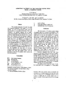
This is not a simple mutual inductive definition of two sets, as B is indexed by A. It is not an ordinary inductive family, as A may refer to B. Finally, it is not an instance of induction-recursion, as B is constructed inductively, not recursively. Let us consider a first example, which will serve as a running example to illustrate the formal rules. We simultaneously define a set of platforms together with buildings constructed on these platforms. The ground is a platform, and if we have a building, we can always construct a new platform from it by building an extension. We can always build a building on top of any platform, and if we have an extension, we can also construct a building hanging from it. (See Figure 1 for an illustration.) This gives rise to the following inductive-inductive definition of Platform ∶ Set, Building ∶ Platform → Set (where p ∶ Platform means that p is a platform and b ∶ Building(p) means that b is a building constructed on the platform p)1 with constructors ground ∶ Platform , extension ∶ ((p ∶ Platform) × Building(p)) → Platform , onTop ∶ (p ∶ Platform) → Building(p) , hangingUnder ∶ ((p ∶ Platform) × (b ∶ Building(p))) → Building(extension(⟨p, b⟩)). Note that the index of the codomain of hangingUnder is extension(⟨p, b⟩), i.e. hangingUnder(⟨p, b⟩) ∶ Building(extension(⟨p, b⟩)). In other words, it is not possible to have a building hanging under the ground.

b b

p

p

p

Fig. 1. onTop(p), extension(⟨p, b⟩) and hangingUnder(⟨p, b⟩). 1

The collection of small types in Martin-L¨ of type theory is called Set for historic reasons, whereas Type is reserved for the collection of large types. The judgement Building ∶ Platform → Set means that for every p ∶ Platform, Building(p) ∶ Set. The type theoretic notation will be further explained in Section 2.

Inductive-inductive definitions have been used by Dybjer [7], Danielsson [5] and Chapman [4] to internalise the syntax and semantics of type theory. Slightly simplified, they define a set Ctxt of contexts, a family Ty ∶ Ctxt → Set of types in a given context, and a family Term ∶ (Γ ∶ Ctxt) → Ty(Γ ) → Set of terms of a given type. Let us for simplicity only consider contexts and types. The set Ctxt of contexts has two constructors ε ∶ Ctxt , cons ∶ ((Γ ∶ Ctxt) × Ty(Γ )) → Ctxt , corresponding to the empty context and extending a context Γ with a new type. In our simplified setting, Ty ∶ Ctxt → Set has the following constructors ’set’ ∶ (Γ ∶ Ctxt) → Ty(Γ ) , Π ∶ ((Γ ∶ Ctxt) × (A ∶ Ty(Γ )) × Ty(cons(⟨Γ, A⟩))) → Ty(Γ ) . The first constructor states that ’set’ is a type in any context. The second constructor Π is the constructor for the Π-type: If we have a type A in a context Γ , and another type B in Γ extended by A (corresponding to abstracting a variable of type A), then Π(A, B) is also a type in Γ . Note how the constructor cons for Ctxt has an argument of type Ty(Γ ), even though Ty is indexed by Ctxt. It is also worth noting that Π has an argument of type Ty(cons(⟨Γ, A⟩)), i.e. we are using the constructor for Ctxt in the index of Ty. In general, we could of course imagine an argument of type Ty(cons(⟨cons(⟨Γ, A⟩), A′ ⟩)) etc. Both Danielsson [5] and Chapman [4] have used the proof assistant Agda [17] as a framework for their formalisation. Agda supports inductive-inductive (and inductive-recursive) definitions via the mutual keyword. However, the theory behind Agda is unclear, especially in relation to mutual definitions. For example, Agda allows the definition of a universe U `a la Tarski, with a code u ∶ U for itself, i.e. T (u) = U . This does not necessarily mean that Agda is inconsistent by Girard’s paradox, as, if we also demand closure under Π or Σ, the positivity checker rejects the code. However the consistency of Agda is by no means clear. Nevertheless, Agda is an excellent tool for trying out ideas. We have formalised our theory in Agda, and this formalisation can be found on the authors’ home pages [14]. Acknowledgements We wish to thank Phillip James and the anonoymous referees of this and previous versions of this article for their helpful comments.

2

Type Theoretic Preliminaries

We work in a type theory with at least two universes Set and Type, with Set ∶ Type and if A ∶ Set then A ∶ Type. Both Set and Type are closed under dependent function types, written (x ∶ A) → B (sometimes denoted (Πx ∶ A)B), where B

is a set or type depending on x ∶ A. Abstraction is written as λx ∶ A.e, where e ∶ B depending on x ∶ A, and application as f (x). Repeated abstraction and application are written as λx1 ∶ A1 . . . xk ∶ Ak .e and f (x1 , . . . , xk ). If the type of x can be inferred, we simply write λx.e as an abbreviation. Furthermore, both Set and Type are closed under dependent sums, written (x ∶ A) × B (sometimes denoted (Σx ∶ A)B), where B is a set or type depending on x ∶ A, with pairs ⟨a, b⟩, where a ∶ A and b ∶ B[x ∶= a]. We also have β- and η-rules for both dependent function types and sums. We need an empty type 0 ∶ Set, with elimination !A ∶ (x ∶ 0) → A for every A ∶ 0 → Set. We need a unit type 1 ∶ Set, with unique element ⋆ ∶ 1. We include an η-rule stating that if x ∶ 1, then x = ⋆ ∶ 1. Moreover, we include a two element set 2 ∶ Set, with elements tt ∶ 2, ff ∶ 2 and elimination constant if ⋅ then ⋅ else ⋅ ∶ (a ∶ 2) → A(tt) → A(ff) → A(a) where A(i) ∶ Type for i ∶ 2. With if ⋅ then ⋅ else ⋅ and dependent products, we can now define the disjoint union of two sets A + B ∶= (x ∶ 2) × (if x then A else B) with constructors inl = λa ∶ A.⟨tt, a⟩ and inr = λb ∶ B.⟨ff, b⟩, and prove the usual formation, introduction, elimination and equality rules. We write A0 + A1 + . . . + An for A0 + (A1 + (. . . + An )⋯) and ink (a) for the kth injection inl(inrk (a)) (with special case inn (a) = inrn (a)). Using (the derived) elimination rules for +, we can, for A, B ∶ Set, C ∶ A+B → Type and f ∶ (a ∶ A) → C(inl(a)), g ∶ (b ∶ B) → C(inr(b)), define the case distinction f ⊔ g ∶ (c ∶ A + B) → C(c) with equality rules (f ⊔ g)(inl(a)) = f (a) , (f ⊔ g)(inr(b)) = g(b) . We will use the same notation even when C does not depend on c ∶ A+B, and we will write f ∥ g ∶ A+B → C +D, where f ∶ A → C, g ∶ B → D, for (inl○f )⊔(inr○g). Intensional type theory in Martin-L¨ of’s logical framework extended with dependent products and 0, 1 and 2 has all the features we need. Thus, our development could, if one so wishes, be seen as an extension of the logical framework.

3

From Inductive to Inductive-inductive Definitions

Let us first, before we move on to inductive-inductive definitions, informally consider how to formalise a simultaneous (generalised) inductive definition of two sets A and B, given by constructors introA ∶ ΦA (A, B) → A

introB ∶ ΦB (A, B) → B

where ΦA and ΦB are strictly positive in the following sense: – The constant Φ(A, B) = 1 is strictly positive. It corresponds to an introduction rule with no arguments (or more precisely, the trivial argument x ∶ 1). – If K is a set and Ψx is strictly positive, depending on x ∶ K, then Φ(A, B) = (x ∶ K)×Ψx (A, B), corresponding to the addition of a non-inductive premise, is strictly positive. So introA has one non-inductive argument x ∶ K, followed by the arguments given by Ψx (A, B).

– If K is a set and Ψ is strictly positive, then Φ(A, B) = (K → A) × Ψ (A, B) is strictly positive. This corresponds to the addition of a premise inductive in A, where K corresponds to the hypothesis of this premise in a generalised inductive definition. So introA has one inductive argument f ∶ K → A, followed by the arguments given by Ψ (A, B). – Likewise, if K is a set and Ψ is strictly positive, then Φ(A, B) = (K → B) × Ψ (A, B) is strictly positive. This is similar to the previous case. In an inductive-inductive definition, B is indexed by A, so the constructor for B is replaced by introB ∶ (a ∶ ΦB (A, B)) → B(iA,B (a)) for some index iA,B (a) ∶ A which might depend on a ∶ ΦB (A, B). Furthermore, we must modify the inductive case for B to specify an index as well. This index can (and usually does) depend on earlier inductive arguments, so that the new inductive cases become – If K is a set, and Ψf is strictly positive, depending2 on f ∶ K → A only in indices for B, then Φ(A, B) = (f ∶ K → A) × Ψf (A, B) is strictly positive. – If K is a set, iA,B ∶ K → A is a function and Ψf is strictly positive, depending on f ∶ (x ∶ K) → B(iA,B (x)) only in indices for B, then Φ(A, B) = (f ∶ ((x ∶ K) → B(iA,B (x)))) × Ψf (A, B) is strictly positive. In what way can the index depend on f ? Before we know the constructor for A, we do not know any functions with codomain A, so the index can only depend directly on f (e.g. B(f (x))). When we define the constructor for B, the situation is similar, but now we know one function into A, namely introA ∶ ΦA (A, B) → A, so that the index could be e.g. introA (f (x), b). (Our approach could also be straightforwardly extended to allow several constructors for A, where later constructors make use of earlier ones.)

4

An Axiomatisation

We proceed as in Dybjer and Setzer [9] and introduce a datatype of codes for constructors. In other words, we define a type SP (for strictly positive) whose elements represent the inductively defined sets, together with a way to construct the real sets from the representing codes. However, as we have two sets A and B with different roles, we need two types SPA and SPB of codes. What do we need to know in order to reconstruct the inductively defined sets? A moment’s thought shows that all we need is the domain of the constructors, and in the case of B, we also need the index of the codomain of the constructor. From this, we can write down the introduction rules, and the elimination rules should be determined by these (see e.g. [6]). Thus, the codes in SPA and SPB will 2

The somewhat vague and informal phrase “depending on f only in indices for B” will be given an exact meaning in the formalisation in the next section.

be codes for the domain of the constructors, and we will have functions ArgA , ArgB that map the code to the domain it represents. For B, there will also be a function IndexB that gives the index (in A) of the codomain of the constructor. We will have special codes A-ind, B-ind for arguments that are inductive in A and B respectively. In the case of B-ind, we also need to specify an index, which might depend on earlier arguments. For instance, the index p of the type of the second argument for the extension constructor extension ∶ ((p ∶ Platform) × Building(p)) → Platform depends on the first argument. How can we specify this index in the code? We cannot make use of the sets A and B themselves, since they are to be defined, but we can refer to their existence. We will introduce parameters Aref , Bref that get updated during the construction of the code. Aref determines the elements of A that we can refer to, and Bref determines the elements b of B, together with the index a such that b ∶ B(a). At the beginning, we cannot refer to any arguments, and so Aref = Bref = 0. For example, after having written down the first argument p ∶ Platform, Aref would be extended to include also an element representing p, which we use when writing down the type of the second argument, Building(p). 4.1

SPA and ArgA

The above discussion leads us to the following formation rule for SPA : Aref ∶ Set Bref ∶ Set SPA (Aref , Bref ) ∶ Type Aref and Bref can be any sets. The codes for inductive-inductive definitions will however be elements from SP′A ∶= SPA (0, 0), i.e. codes that do not refer to any elements to start with. The introduction rules for SPA reflect the rules for strict positivity in Section 3. The rules are as follows (we suppress the global premise Aref , Bref ∶ Set): nilA ∶ SPA (Aref , Bref )

K ∶ Set γ ∶ K → SPA (Aref , Bref ) nonind(K, γ) ∶ SPA (Aref , Bref )

K ∶ Set γ ∶ SPA (Aref + K, Bref ) K ∶ Set hindex ∶ K → Aref γ ∶ SPA (Aref , Bref + K) A-ind(K, γ) ∶ SPA (Aref , Bref ) B-ind(K, hindex , γ) ∶ SPA (Aref , Bref ) The code nilA represents a trivial constructor (the base case). The code nonind(K, γ) is meant to represent a noninductive argument x ∶ K, with the rest of the arguments given by γ(x). The code A-ind(K, γ) is meant to represent a (generalised) inductive argument of type K → A, with the rest of the arguments given by γ. Finally, the code B-ind(K, hindex, γ) represents an inductive argument of type (x ∶ K) → B(i(x)), where the index i(x) is determined by hindex , and the rest of the arguments are given by γ. For instance, a constructor c ∶ ((x ∶ 2) × (N → A)) → A

has the code γc = nonind(2, λx.A-ind(N, nilA )). Note how 2 and N appear in the code. We will see an example of the slightly more complicated constructor B-ind later. We will now define ArgA , which maps a code to the domain of the constructor it represents. ArgA will need to take arbitrary A ∶ Set and B ∶ A → Set as parameters to use as A and B in the inductive arguments, since we need ArgA to define the A and B we want. We will then have axioms stating that for every code γ ∶ SP′A , there are sets Aγ , Bγ closed under ArgA , i.e. there is a constructor introA ∶ ArgA (γ, Aγ , Bγ ) → Aγ . ArgA has formation rule repA ∶ Aref → A rep Aref , Bref ∶ Set index ∶ Bref → A A ∶ Set γ ∶ SPA (Aref , Bref ) B ∶ A → Set repB ∶ (x ∶ Bref ) → B(repindex (x)) ArgA (Aref , Bref , γ, A, B, repA , repindex , repB ) ∶ Set The function repA translates elements in Aref into the real elements they represent in A. Elements in Bref represent elements b from B, but also elements from A, as we also need to store the index a such that b ∶ B(a). This index is given by repindex, and repB gives the real element in B(repindex (y)) an element y ∶ Bref represents. We are actually only interested in ArgA for codes γ ∶ SP′A for inductiveinductive definitions (i.e. with Aref = Bref = 0), but we need to consider arbitrary Aref , Bref for the intermediate codes. For γ ∶ SP′A , we can define a simplified version Arg′A ∶ SP′A → (A ∶ Set) → (B ∶ A → Set) → Set by Arg′A (γ, A, B) ∶ = ArgA (0, 0, γ, A, B, !A , !A , !B○!A ). (Recall that !X ∶ (x ∶ 0) → X is the function given by ex falso quodlibet.) The definition of ArgA also follows the rules for strict positivity in Section 3. We will, for readability, write “ ” for arguments which are simply passed on in the recursive call. The code nilA represents the constructor with no argument (i.e. a trivial argument of type 1): ArgA (Aref , Bref , nilA , A, B, repA , repindex , repB ) = 1 The code nonind(K, γ) represents one non-inductive argument k ∶ K, with the rest of the arguments given by the code γ (depending on k ∶ K): ArgA (Aref , Bref , nonind(K, γ), A, B, repA , repindex , repB ) = (k ∶ K) × ArgA ( , , γ(k), , , , , ) The code A-ind(K, γ) represents one generalised inductive argument j ∶ K → A, with the rest of the arguments given by the code γ. In the following arguments, Aref has now been updated to Aref +K, where elements in the old Aref are mapped to A by the old repA , and elements in K are mapped to A by j. In effect, this means that we can refer to j(k) for k ∶ K in the following arguments. ArgA (Aref , Bref , A-ind(K, γ), A, B, repA , repindex, repB ) = (j ∶ K → A) × ArgA (Aref + K, , γ, , , repA ⊔ j, , )

Finally, the code B-ind(K, hindex , γ) represents one generalised inductive argument j ∶ (x ∶ K) → B((repA ○ hindex)(x)), where repA ○ hindex picks out the index of the type of j(x). This time, we can refer to more elements in B afterwards, namely those given by j (and indices given by repA ○ hindex): ArgA (Aref , Bref , B-ind(K, hindex, γ), A, B, repA , repindex , repB ) = (j ∶ (k ∶ K) → B((repA ○ hindex )(k)))× ArgA ( , Bref + K, γ, , , , repindex ⊔ (repA ○ hindex), repB ⊔ j) Let us take a look at the constructor extension ∶ ((p ∶ Platform) × Building(p)) → Platform again. It would have the code γext = A-ind(1, B-ind(1, λ ⋆ .ˆ p, nilA )) ∶ SP′A where pˆ = inr(⋆) is the element in Aref = 0 + 1 representing the element introduced by A-ind. We have Arg′A (γext , Platform, Building) = (p ∶ 1 → Platform) × (1 → Building(p(⋆))) × 1 which is isomorphic to the domain of extension thanks to the η-rules for 1 (i.e. X ≅ 1 → X and X ≅ X × 1). 4.2

Towards SPB

If we did not want to use constructors for A as indices for B, like for example Building(extension(⟨p, b⟩)), we could construct SPB in more or less the same way as SPA (this corresponds to choosing k = 0 below). However, in general we do want to use constructors as indices, hence we have some more work to do. What do we need to know for such a constructor index? We need to know that we want to use a constructor, but that can be encoded in the code. We also need a way to specify the arguments to the constructor, i.e. we need to represent an element of Arg′A (γ, A, B)! If we want to use nested constructors (e.g. extension(⟨extension(⟨p, b⟩), b′ ⟩)), we also need to be able to represent elements in Arg′A (γ, Arg′A (γ, A, B0 ), B1 ) etc. The idea is to represent elements in Arg′A (γ, A, B) by corresponding elements in “Arg′A (γ, Aref , Bref )”. However, we must first reconstruct the structure of Aref , Bref as a family, i.e. we will construct Aref ∶ Set, Bref ∶ Aref → Set, together with functions repA ∶ Aref → A and repB ∶ (x ∶ Aref ) → Bref (x) → B(repA (x)). Then, we will show that repA and repB can be lifted to a map lift′ (repA , repB ) ∶ Arg′A (γ, Aref , Bref ) → Arg′A (γ, A, B), so that elements in Arg′A (γ, Aref , Bref ) indeed can represent elements in Arg′A (γ, A, B). The process can then be iterated to represent elements in Arg′A (γ, Arg′A (γ, A, B0 ), B1 ) etc. Aref should consist of representatives a for elements a in A, and Bref (a) should consist of representatives for elements in B(a). The representative a could either be from Aref (with a = repA (a)), in which case we do not know any elements

in B(a), or from Bref (with a = repindex(a)), in which case we know a single element in B(a), namely repB (a). Therefore, for Aref , Bref ∶ Set, we define

Aref ∶= Aref + Bref ,

Bref ∶= (λx.0) ⊔ (λx.1) ,

i.e. Bref (inl(a)) = 0 and Bref (inr(b)) = 1. Mapping representatives in Aref to the elements they represent in A is now easy: we map inl(a) ∶ Aref to repA (a) and inr(a) to repindex (a). For Bref , we want to map representatives in Bref (a) to the elements they represent in B(a). However, we only have to consider Bref (inr(x)) = 1, as there are no elements in Bref (inl(x)) = 0. We map ⋆ ∶ Bref (inr(a)) to repB (a). To sum up, we can define maps repA ∶ Aref → A, repB ∶ (x ∶ Aref ) → Bref (x) → B(repA (x)) by repA ∶= repA ⊔ repindex and repB ∶= (λx.!B○!A ) ⊔ (λx ⋆ .repB (x)). We now want to lift these maps to a map repA,1 ∶ Arg′A (γ, Aref , Bref ) → Arg′A (γ, A, B). This is made possible by the following more general result for arbitrary families A, B, A∗ , B ∗ with respective representing functions repA , rep∗A etc. Assume we have maps g ∶ A → A∗ , g ′ ∶ (x ∶ A) → B(x) → B ∗ (g(x)) that respect the translations repA and rep∗A , i.e. we have a proof p that g(repA (x)) = rep∗A (x) for all x ∶ Aref . Then we can lift g to a map

lift(g, g ′ , p) ∶ ArgA (Aref , Bref , γ, A, B, repA , repindex, repB ) → ArgA (Aref , Bref , γ, A∗ , B ∗ , rep∗A , rep∗index , rep∗B ) .

To avoid using the identity type when constructing lift, we will use a specialised version of Leibniz equality p ∶ (x ∶ Aref ) → B ∗ (g(repA (x))) → B ∗ (rep∗A (x)) for the proof that g(repA (x)) = rep∗A (x). Under the assumption that γ ∶ SPA (Aref , Bref ) , and with A, B, repA , repindex , repB as above, and A∗ , B ∗ , rep∗A , rep∗index, rep∗B analogously, we now have formation rule

lift(Aref , Bref , γ, A, B, repA , repindex, repB , A∗ , B ∗ , rep∗A , rep∗index, rep∗B ) ∶ (g ∶ A → A∗ ) → (g ′ ∶ (x ∶ A) → B(x) → B ∗ (g(x))) → (p ∶ (x ∶ Aref ) → B ∗ (g(repA (x))) → B ∗ (rep∗A (x))) → ArgA (Aref , Bref , γ, A, B, repA , repindex , repB ) → ArgA (Aref , Bref , γ, A∗ , B ∗ , rep∗A , rep∗index , rep∗B )

with defining equations (we write “ ” for passed on arguments in the recursive call) lift(Aref , Bref , nilA , repA , repindex , repB , rep∗A , rep∗index, rep∗B , g, g ′ , p, ⋆) = ⋆ lift(Aref , Bref , nonind(K, γ), repA , repindex, repB , rep∗A , rep∗index, rep∗B , g, g ′ , p, ⟨k, y⟩) = ⟨k, lift( , , γ(k), , , , , , , , , , y)⟩ lift(Aref , Bref , A-ind(K, γ), repA , repindex , repB , rep∗A , rep∗index , rep∗B , g, g ′ , p, ⟨j, y⟩) = ⟨g ○ j, lift(Aref + K, , γ, repA ⊔ j, , , rep∗A ⊔ (g ○ j), , , , , p ⊔ (λk, b.b), y)⟩ lift(Aref , Bref , B-ind(K, hindex, γ), repA , repindex , repB , rep∗A , rep∗index , rep∗B , g, g ′ , p, ⟨j, y⟩) = ⟨λk.p(hindex (k), g ′ (repA ○ hindex (k)), j(k))), lift( , Bref + K, γ, , repindex ⊔ (repA ○ hindex ), repB ⊔ j, , rep∗index ⊔ (rep∗A ○ hindex ), rep∗B ⊔ (λk.p(hindex(k), g ′ (repA (hindex(k)), j(k)))), , , , y)⟩. Note how the proof p ∶ (x ∶ Aref ) → B ∗ (g(repA (x))) → B ∗ (rep∗A (x)) gets updated to p ⊔ (λk b.b) when Aref is extended to Aref + K. For γ ∶ SP′A , g ∶ A → A∗ , g ′ ∶ (x ∶ A) → B(x) → B ∗ (g(x)), we define lift′ (γ, A, B, A∗ , B ∗ , g, g ′ ) ∶ Arg′A (γ, A, B) → Arg′A (γ, A∗ , B ∗ ) by lift′ (γ, A, B, A∗ , B ∗ , g, g ′ , a) ∶= lift(0, 0, γ, A, B, !A , !A , !B○!A , A∗ , B ∗ , !A∗ , !A∗ , !B ∗ , g, g ′ , triv, a). where triv ∶ (x ∶ 0) → B ∗ (g(repA (x)) → B ∗ (rep∗A (x)) is the trivial proof supplied by ex falso quodlibet. In our specific case, let for γ ∶ SP′A , Aref , Bref ∶ Set and repA ∶ Aref → A, repindex ∶ Bref → A, repB ∶ (b ∶ Bref ) → B(repindex (b)) argA (γ, Aref , Bref ) ∶= Arg′A (γ, Aref , Bref ) , lift(repA , repindex , repB ) ∶= lift′ (repA , repB ) ∶ argA (γ, Aref , Bref ) → Arg′A (γ, A, B) . We can now represent elements in Arg′A (γ, A, B) by elements in argA (γ, Aref , Bref ) via repA,1 ∶= lift(repA , repindex , repB ). For example, consider γext once again. Suppose that we want to specify an element of Arg′A (γext , Platform, Building), i.e. an argument to the extension constructor, and we have Aref = Bref = 0 + 1. Aref then ̂ = inr(inr(⋆)). We have consists of two elements, namely pˆ = inl(inr(⋆)) and pb ̂= ̂ that Bref (ˆ p) = 0 and Bref (pb) = 1. In other words, there is only one element ⟨pb⟩ ′ ̂ = ⟨rep ̂ ⋆, ⋆⟩ of Arg (γext , Aref , Bref ), and rep (⟨pb⟩) ̂ ̂ ⟨pb, A A,1 index (pb), repB (pb), ⋆⟩ = ̂ ̂ ⟨p, b, ⋆⟩ where repindex (pb) = p ∶ Platform, repB (pb) = b ∶ Building(p). Let us now generalise this to multiple nestings of constructors. Given a se⃗ref(n) = Bref, 0 , Bref, 1 , . . . , Bref, n − 1 of sets, we iterate arg by defining quence B A ⃗ref(0) ) = Aref , arg0A (γ, Aref , B n i ⃗ ⃗ argn+1 A (γ, Aref , Bref(n+1) ) = argA (γ, + argA (γ, Aref , Bref(i) ), Bref, n ) . i=0

argkA should represent k nested constructors. The corresponding iteration of Arg′A justifying this, is ⃗(0) ) = A , Arg0A (γ, A, B n n ′ i ⃗ ⃗ Argn+1 A (γ, A, B(n+1) ) = ArgA (γ, + ArgA (γ, A, B(i) ), ⊔ Bi ) , i=0

i=0

⃗(i−1) ) ArgiA (γA , A, B

⃗(n) is a sequence B0 , B1 , . . . , Bn−1 of families Bi ∶ where B → Set. ⃗ref(n) of sets and a sequence B ⃗(n) Now assume that we have a sequence B of families of sets as above. If we now in addition to repA ∶ Aref → A, also ⃗ and repB,i ∶ (x ∶ Bref, i ) → have functions repindex,i ∶ Bref, i → ArgiA (γ, A, B), Bi (repindex,i (x)) (we will assume all this when working with SPB ), we can now ⃗ref ) → Argn (γ, A, B) ⃗ with the help of construct functions repA,n ∶ argnA (γ, Aref , B A ′ lift by defining repA,0 repA,n+1

= repA , n n = lift( repA,i , inn ○ repindex,n , repB,n ) . i=0

Note that repA,1 as defined earlier is an instance of this definition. 4.3

SPB , ArgB and IndexB

The datatype SPB of codes for constructors for B is just as SPA , but with two differences: first, we can refer to constructors of A (so we will need a code γA ∶ SP′A to know their form, and sets Bref, 0 , Bref, 1 , . . . Bref, i , . . . to represent elements in B indexed by i nested constructors). Second, we also need to specify an index for the codomain of the constructor (so we will store this index in the nilB code). All constructions from now on will be parameterised on the maximum number k of nested constructors for A that we are using, so we are really introducing SPB,k , ArgB,k etc. However, we will work with an arbitrary k but suppress it as a premise. With this in mind, we have formation rule γA ∶ SP′A Aref ∶ Set Bref, 0 , Bref, 1 , . . . , Bref, k ∶ Set SPB (γA , Aref , Bref, 0 , Bref, 1 , . . . , Bref, k ) ∶ Type Let SP′B (γA ) ∶= SPB (γA , 0, 0, . . . , 0) for γA ∶ SP′A be the code of inductiveinductive definitions. The introduction rules for SPB are very similar to the rules for SPA , but now we specify an index in nilB , and we have k + 1 rules B0 -ind, . . . , Bk -ind corresponding to how many nested constructors for A we want to use: ⃗ref ) aindex ∶ +ki=0 argiA (γA , Aref , B nilB (aindex ) ∶ SPB (γA , Aref , Bref, 0 , . . . , Bref, k )

K ∶ Set γ ∶ K → SPB (γA , Aref , Bref, 0 , . . . , Bref, k ) nonind(K, γ) ∶ SPB (γA , Aref , Bref, 0 , . . . , Bref, k ) K ∶ Set γ ∶ SPB (γA , Aref + K, Bref, 0 , . . . , Bref, k ) A-ind(K, γ) ∶ SPB (γA , Aref , Bref, 0 , . . . , Bref, k ) ⃗ref ) hindex ∶ K → arg`A (γA , Aref , B K ∶ Set γ ∶ SPB (γA , Aref , Bref, 0 , . . . , Bref, ` + K, . . . , Bref, k ) B` -ind(K, hindex, γ) ∶ SPB (γA , Aref , Bref, 0 , . . . , Bref, k ) The rules nilB , nonind and A-ind have the same meaning as before, but B-ind has been split up into several rules. The code B` -ind(K, hindex , γ) represents an inductive argument of type (x ∶ K) → B(i` (x)) with the index i` (x), using ` nested constructors for A, given by hindex. Hence hindex has codomain ⃗ref ). For this to work, we will need k+1 families Bi ∶ ArgiA (γA , A, B ⃗(i−1) ) → arg`A (γA , Aref , B Set to interpret these nested constructor indices, together with functions repindex,i ∶ ⃗(i−1) ) and repB,i ∶ (x ∶ Bref, i ) → Bi (repindex,i (x)) to map Bref, i → ArgiA (γ, A, B elements to the real elements they represent. Recall that from this and repA ∶ ⃗ref ) → Arg` (γ, A, B). ⃗ Aref → A, we can construct functions repA,` ∶ arg`A (γ, Aref , B A Every case of ArgB is the same as the corresponding case for ArgA , except for B` -ind, where B has been replaced by B` and repA by repA,` (we write “ ” for passed on arguments and “ ” for passed on sequents of arguments in the recursive call): ⃗ref , nilB (aindex ), A, B, ⃗ repA , rep ArgB (γA , Aref , B ⃗ index, rep ⃗ B) = 1 ⃗ref , nonind(K, γ), A, B, ⃗ rep , rep Arg (γA , Aref , B ⃗ , rep ⃗ )= B

A

index

B

(k ∶ K) × ArgB ( , , , γ(k), , , , , ) ⃗ref , A-ind(K, γ), A, B, ⃗ repA , rep ArgB (γA , Aref , B ⃗ index , rep ⃗ B) = (j ∶ K → A) × ArgB ( , Aref + K, , γ, , , repA ⊔ j, , ) ⃗ ⃗ repA , rep ArgB (γA , Aref , Bref , B` -ind(K, hindex , γ), A, B, ⃗ index , rep ⃗ B) = (j ∶ (k ∶ K) → B` ((repA,` ○ hindex)(k))) × ArgB ( , , , Bref, ` +K, , γ, , , , , repindex,` ⊔(repA,` ○hindex), , , repB,` ⊔j, ) ⃗ The last missing piece is now IndexB , which to each b ∶ Arg′B (γA , γB , A, B) assigns the index a such that the element constructed from b is in B(a). With γA , Aref , Bref, i etc as above, IndexB has formation rule ⃗ref , γB , A, B, ⃗ repA , rep IndexB (γA , Aref , B ⃗ index , rep ⃗ B) ∶

k

⃗ref , γB , A, B, ⃗ repA , rep ⃗ ArgB (γA , Aref , B ⃗ index, rep ⃗ B ) → + ArgiA (γA , A, B). i=0

⃗ref ) which is stored in nilB and map IndexB will take aindex ∶ +ki=0 argiA (γA , Aref , B ⃗ For other codes, it it to the index element it represents in +ki=0 ArgiA (γA , A, B).

will follow exactly the same pattern as ArgB . ⃗ref , nilB (aindex), A, B, ⃗ repA , rep IndexB (γA , Aref , B ⃗ index , rep ⃗ B , ⋆) = (

nk

repA,i )(aindex )

i=0

⃗ref , nonind(K, γ), A, B, ⃗ rep , rep IndexB (γA , Aref , B ⃗ B , ⟨k, y⟩) = A ⃗ index , rep IndexB ( , , , γ(k), , , , , , y) ⃗ ⃗ IndexB (γA , Aref , Bref , A-ind(K, γ), A, B, repA , rep ⃗ index , rep ⃗ B , ⟨j, y⟩) = IndexB ( , Aref + K, , γ, , , repA ⊔ j, , , y) ⃗ ⃗ repA , rep IndexB (γA , Aref , Bref , Bn -ind(K, h, γ), A, B, ⃗ index , rep ⃗ B , ⟨j, y⟩) = IndexB ( , , , Bref, n +K, , γ, , , , , repindex,n ⊔(repA,n ○h), , , repB,n ⊔j, , y). For codes γB ∶ SP′B (γA ) for inductive-inductive definitions, let ⃗ , !B○! ⃗ ) , ⃗ ∶= Arg (γA , 0, 0, ⃗ !A , !Arg ⃗ γB , A, B, Arg′B (γA , γB , A, B) B A ⃗ ) . ⃗ , !B○! ⃗ ∶= IndexB (γA , 0, 0, ⃗ !A , !Arg ⃗ γB , A, B, Index′B (γA , γB , A, B) A As an illustration, let us consider the constructor hangingUnder ∶ ((p ∶ Platform)×(b ∶ Building(p))) → Building(extension(⟨p, b⟩)) . Here it is interesting to see that the index of the codomain of the constructor uses the constructor extension, so it will be represented by an element from argA (γext , Aref , Bref ). We end up with the code γhu = A-ind(1, B0 -ind(1, λ ⋆ .ˆ p, ̂ ̂ = ⟨inr(inr(⋆)), ⋆, ⋆⟩. (The reader is nilB (in1 (⟨pb⟩)))), where pˆ = inr(⋆) and ⟨pb⟩ ̂ ∶ arg (γext , Aref , Bref ) at that point in the construction invited to check that ⟨pb⟩ A of γhu .) We get Arg′B (γext , γhu , P, B) = (p ∶ 1 → P ) × (b ∶ 1 → B(p(⋆))) × 1 and Index′B (γext , γhu , P, B, ⟨p, b, ⋆⟩) = in1 (⟨p, b, ⋆⟩). 4.4

Formation and Introduction Rules

We are now ready to give the formal formation and introduction rules for A and B. They all have the common premises γA ∶ SP′A and γB ∶ SP′B (γA ), which will be omitted. Formation rules: AγA ,γB ∶ Set ,

BγA ,γB ∶ AγA ,γB → Set .

Introduction rule for AγA ,γB : a ∶ Arg′A (γA , AγA ,γB , BγA ,γB ) introA (a) ∶ AγA ,γB

For the introduction rule for BγA ,γB , we need some preliminary definitions. We ⃗(i−1) ) → Set for have BγA ,γB ∶ AγA ,γB → Set, but need Bi ∶ ArgiA (γA , AγA ,γB , B 0 ≤ i ≤ k to give to Arg′B . We can assemble such Bi ’s from BγA ,γB , introA and lift′ . To do so, define in a step by step manner intron ∶ ArgnA (γA , AγA ,γB , B0 , . . . , Bn−1 ) → AγA ,γB Bn ∶ ArgnA (γA , AγA ,γB , B0 , . . . , Bn−1 ) → Set (i.e. introduce first intro0 , B0 , then intro1 , B1 and so on) by intro0 = id

n

n

i=0

i=0

intron+1 = introA ○ lift′ ( ⊔ introi , ⊔ (λa.id)) Bi (x) = BγA ,γB (introi (x)) Hence the introduction rule for BγA ,γB can be given as: b ∶ Arg′B (γA , γB , AγA ,γB , BγA ,γB , B1 , . . . , Bk ) introB (b) ∶ BγA ,γB (index(b)) ⃗ returned by Index′B where index takes the index in +ki=1 ArgiA (γA , AγA ,γB , B) and applies the right introi to it, i.e. k

index = ( ⊔ introi ) ○ Index′B (γA , γB , AγA ,γB , B0 , . . . , Bk ) . i=0

4.5

Elimination rules

The intuitive idea behind the elimination rules is the following: we have E ∶ A → Set and E ′ ∶ (a ∶ A) → B(a) → Set, and would like to construct functions f ∶ (a ∶ A) → E(a) and g ∶ (a ∶ A) → (b ∶ B(a)) → E ′ (a, b). f and g might very well be mutually recursive, since A and B are mutually defined. The elimination rules now state that if we can define functions f ′ ∶ (a ∶ Arg′A (γA , A, B)) → E(introA (a)) and g ′ ∶ (b ∶ Arg′B (γA , γB , A, B)) → E ′ (index(b), introB (b)), given that we already know the value of (mutual) recursive calls, we have functions f ∶ (a ∶ A) → E(a) and g ∶ (a ∶ A) → (b ∶ B(a)) → E ′ (a, b). To this end, let us define sets IHA and IHB of inductive hypotheses, together ⃗ → with maps mapIHA ∶ Arg′A (γA , A, B) → IHA , mapIHB ∶ Arg′B (γA , γB , A, B) IHB which take care of the recursive call. More specifically, if Aref , Bref , γA , A, B, repA , repindex , repB are as in the premises for ArgA , and E ∶ A → Set, E ′ ∶ (a ∶ A) → B(a) → Set, then IHA (Aref , Bref , γA , A, B, repA , repindex , repB , E, E ′ ) ∶ ArgA (Aref , Bref , γA , A, B, repA , repindex , repB ) → Set

and mapIHA (Aref , Bref , γA , A, B, repA , repindex, repB , E, E ′ ) ∶ (R ∶ (a ∶ A) → E(a)) → (R′ ∶ (a ∶ A) → (b ∶ B(a)) → E ′ (a, b)) → (a ∶ ArgA (Aref , Bref , γA , A, B, repA , repindex, repB )) → IHA (Aref , Bref , γA , A, B, repA , repindex , repB , E, E ′ , a). IHA is defined as follows:

IHA (Aref , Bref , nilA , A, B, repA , repindex , repB , E, E ′ , ⋆) = 1 IHA (Aref , Bref , nonind(K, γ), A, B, repA , repindex , repB , E, E ′ , ⟨k, y⟩) = IHA ( , , γ(k), , , , , , , , y) IHA (Aref , Bref , A-ind(K, γ), A, B, repA , repindex, repB , E, E ′ , ⟨j, y⟩) = ((k ∶ K) → E(j(k))) × IHA (Aref + K, , γ, , , repA ⊔ j, , , , , y) IHA (Aref , Bref , B-ind(K, hindex , γ), A, B, repA , repindex , repB , E, E ′ , ⟨j, y⟩) = ((k ∶ K) → E ′ ((repA ○ hindex )(k), j(k)))× IHA ( , Bref + K, γ, , , , repindex ⊔ (repA ○ hindex ), repB ⊔ j, , , y) . mapIHA maps a ∶ ArgA (γA , A, B) to IHA (γA , A, B, a), given that we have functions R, R′ for the recursive calls. It has the following defining equations: mapIHA (Aref , Bref , nilA , A, B, repA , repindex , repB , E, E ′ , R, R′ , ⋆) = ⋆ mapIHA (Aref , Bref , nonind(K, γ), A, B, repA , repindex , repB , E, E ′ , R, R′ , ⟨k, y⟩) = mapIHA ( , , γ(k), , , , , , , , , , y) mapIHA (Aref , Bref , A-ind(K, γ), A, B, repA , repindex, repB , E, E ′ , R, R′ , ⟨j, y⟩) = ⟨R ○ j, mapIHA (Aref + K, , γ, , , repA ⊔ j, , , , , , , y)⟩ mapIHA (Aref , Bref , B-ind(K, h, γ), A, B, repA , repindex , repB , E, E ′ , R, R′ , ⟨j, y⟩) = ⟨λk.R′ (repA (h(k)), j(k)), mapIHA ( , Bref + K, γ, , , , repindex ⊔ (repA ○ h), repB ⊔ j, , , , , y)⟩ . We now repeat the process for IHB and mapIHB . This time, however, we ⃗ have not one B ∶ A → Set but k + 1 families Bi ∶ Arg′i A (γA , A, B(i−1) ) → Set, so we ′i ⃗ → Bi (a) → Set and k + 1 functions need k + 1 families Ei′ ∶ (a ∶ ArgA (γA , A, B)) ⃗ Ri′ ∶ (a ∶ Arg′i (γ , A, B)) → (b ∶ B (a)) → Ei′ (a, b). Otherwise, the pattern is the i A A same. The formation rules are as follows: if γA , Aref , Bref, i , γB , A, Bi , repA , ′ ′ ⃗ fA,i ,fB,i are as before, and E ∶ A → Set, Ei′ ∶ (a ∶ Arg′i A (γA , A, B(i−1) )) → Bi (a) → Set, then ⃗ref , γA , A, B, ⃗ rep , rep IHB (γA , Aref , B ⃗ B , E, E⃗′ ) ∶ A ⃗ index , rep ⃗ref , γB , A, B, ⃗ rep , rep Arg (γA , Aref , B ⃗ B

and

A

⃗ B) index , rep

→ Set

⃗ref , γB , A, B, ⃗ rep , rep mapIHB (γA , Aref , B ⃗ B , E, E⃗′ ) ∶ A ⃗ index , rep (R ∶ (a ∶ A) → E(a)) → (R0′ ∶ (a ∶ A) → (b ∶ B0 (a)) → E0′ (a, b)) → ′ (R1′ ∶ (a ∶ Arg′1 A (γA , A, B0 )) → (b ∶ B1 (a)) → E1 (a, b)) →

⋮ (Rk′

Arg′k A (γA , A, Bk−1 ))

→ (b ∶ Bk (a)) → Ek′ (a, b)) → ⃗ref , γB , A, B, ⃗ rep , rep (b ∶ ArgB (γA , Aref , B ⃗ B )) → A ⃗ index , rep ⃗ref , γB , A, B, ⃗ repA , rep IHB (γA , Aref , B ⃗ index , rep ⃗ B , E, E⃗′ , b). ∶ (a ∶

We get the equations for IHB and mapIHB by changing IHA and mapIHA in more or less the same way we changed ArgA to get ArgB ; in the Bn -ind case, we replace repA with repA,n , repindex with repindex,n , repB with repB,n , B with Bn and now also E ′ with En′ and R′ with Rn′ . ⃗ref , nilB (d), A, B, ⃗ rep , rep IHB (γA , Aref , B ⃗ B , E, E⃗ ′ , ⋆) = 1 A ⃗ index , rep ′ ⃗ ⃗ ⃗ IHB (γA , Aref , Bref , nonind(K, γ), A, B, repA , rep ⃗ index , rep ⃗ B , E, E , ⟨k, y⟩) = IHB ( , , , γ(k), , , , , , , , y) ⃗ref , A-ind(K, γ), A, B, ⃗ repA , rep IHB (γA , Aref , B ⃗ index, rep ⃗ B , E, E⃗ ′ , ⟨j, y⟩) = ((k ∶ K) → E(j(k))) × IHB ( , Aref + K, , γ, , , repA ⊔ j, , , , , y) ⃗ref , Bn -ind(K, h, γ), A, B, ⃗ rep , rep IHB (γA , Aref , B ⃗ B , E, E⃗ ′ , ⟨j, y⟩) = A ⃗ index , rep ′ ((k ∶ K) → En (repA,n (h(k)), j(k)))× ′ ⊔ j, , , , y). IHB ( , , , Bref, n + K, , γ, , , , , repindex,n ⊔ (repA,n ○ h), , , fB,n ⃗ref , nilB (d), A, B, ⃗ rep , rep ⃗ ′ , R, R⃗′ , ⋆) mapIHB (γA , Aref , B ⃗ B , E, E = ⋆ A ⃗ index , rep ⃗ref , nonind(K, γ), A, B, ⃗ repA , rep mapIHB (γA , Aref , B ⃗ index , rep ⃗ B , E, E⃗ ′ , R, R⃗′ , ⟨k, y⟩) = mapIHB ( , , , γ(k), , , , , , , , , , y) ⃗ref , A-ind(K, γ), A, B, ⃗ repA , rep mapIHB (γA , Aref , B ⃗ index , rep ⃗ B , E, E⃗ ′ , R, R⃗′ , ⟨j, y⟩) = ⟨R ○ j, mapIHB ( , Aref + K, , γ, , , repA ⊔ j, , , , , , , y)⟩ ⃗ref , Bn -ind(K, h, γ), A, B, ⃗ repA , rep mapIHB (γA , Aref , B ⃗ index , rep ⃗ B , E, E⃗ ′ , R, R⃗′ , ⟨j, y⟩) = ′ ⟨λk.Rn (repA,n (h(k)), j(k)), mapIHA ( , , , Bref, n + K, , γ, , , , , repindex,A,n ⊔ (repA,n ○ h), , , repB,B,n ⊔ j, , , , , , y)⟩. We make the usual abbreviations IH’A (γA , A, B, E, E ′ , a) ∶= IHA (0, 0, γA , A, B, !A , !A , !B○! , E, E ′ , a) mapIH′A (γA , A, B, E, E ′ , R, R′ , a) ∶= mapIHA (0, 0, γA , A, B, !A , !A , !B○! , E, E ′ , R, R′ , a)

⃗ E, E⃗′ , b) ∶= IH’B (γA , γB , A, B, ⃗ , E, E⃗′ , b) ⃗ !A , !Arg , !B○! ⃗ γB , A, B, IHB (γA , 0, 0, A ⃗ E, E⃗′ , R, R⃗′ , b) ∶= mapIH′ (γA , γB , A, B, B

⃗ , E, E⃗′ , R, R⃗′ , b). ⃗ !A , !Arg , !B○! ⃗ γB , A, B, mapIHB (γA , 0, 0, A It is now time to introduce the elimination and equality rules for AγA ,γB and BγA ,γB . We have used the abbreviations Bn from Section 4.4, as well as a new abbreviation En′ ∶= λa, b.E ′ (intron (a), b). For E ∶ AγA ,γB → Set and E ′ ∶ (a ∶ AγA ,γB ) → BγA ,γB (a) → Set, we have elimination rules (we have abbreviated A ∶= AγA ,γB , B ∶= BγA ,γB ) g ∶ (a ∶ Arg′A (γA , A, B)) → IH’A (γA , A, B, E, E ′ , a) → E(introA (a)) ⃗ E, E ′ , . . . , E ′ , b) → E ′ (index(b), introB (b)) h ∶ (b ∶ Arg′B (γA , γB , A, B0 , . . . , Bk )) → IH’B (γA , γB , A, B, 0 k RA (g, h) ∶ (a ∶ AγA ,γB ) → E(a) h ∶ (b ∶

g ∶ (a ∶ Arg′A (γA , A, B)) → IH’A (γA , A, B, E, E ′ , a) → E(introA (a)) ′ ⃗ E, E ′ , . . . , E ′ , b) → E ′ (index(b), introB (b)) ArgB (γA , γB , A, B0 , . . . , Bk )) → IH’B (γA , γB , A, B, 0 k RB (g, h) ∶ (a ∶ AγA ,γB ) → (b ∶ BγA ,γB (a)) → E ′ (a, b) with equality rules (premises omitted) RA (g, h, introA (a)) = g(a, mapIH′A (γA , A, B, E, E ′ , RA (g, h), RB (g, h), a)) ⃗ E, E⃗ ′ , RA (g, h), RB (g, h), b)) RB (g, h, index(b), introB (b)) = h(b, mapIH′B (γA , γB , A, B, 4.6

Contexts and Types Again

As a final example, let us construct Ctxt and Ty from Section 1. With the abbreviation γ0 +SP γ1 ∶= nonind(2, λx.if x then γ0 else γ1 ), we can encode several constructors into one. The codes for the contexts and types are γCtxt = nilA +SP A-ind(1, B-ind(1, λ ⋆ .inr(⋆), nilA )) ∶ SP′A γ’set’ = A-ind(1, nilB (inl(inr(⋆)))) γΠ = A-ind(1, B0 -ind(1, λ ⋆ .inr(⋆), B1 -ind(1, λ ⋆ .⟨ff, ⟨λ ⋆ .inr(inr(⋆)), ⟨λ ⋆ .⋆, ⋆⟩⟩⟩, nilB (inl(inr(⋆)))))) γTy = γ’set’ +SP γΠ ∶ SP′B (γCtxt ) . We have Ctxt = AγCtxt ,γTy and Ty = BγCtxt ,γTy and we can define the usual constructors by ε ∶ Ctxt ε = introA ⟨tt, ⋆⟩ ,

’set’ ∶ (Γ ∶ Ctxt) → Ty(Γ ) ’set’(Γ ) = introB ⟨tt, ⟨(λ ⋆ .Γ ), ⋆⟩⟩ ,

cons ∶ (Γ ∶ Ctxt) → Ty(Γ ) → Ctxt cons(Γ, b) = introA (⟨ff, ⟨(λ ⋆ .Γ ), ⟨(λ ⋆ .b), ⋆⟩⟩⟩) , Π ∶ (Γ ∶ Ctxt) → (A ∶ Ty(Γ )) → Ty(cons(Γ, A)) → Ty(Γ ) Π(Γ, A, B) = introB (⟨ff, ⟨(λ ⋆ .Γ ), ⟨(λ ⋆ .A), ⟨(λ ⋆ .B), ⋆⟩⟩⟩⟩) .

5

A Set-theoretic Model

Even though SPA and SPB are straightforward (large) inductive definitions, this axiomatisation does not reduce inductive-inductive definitions to indexed inductive definitions, since the formation and introduction rules are not instances of ordinary indexed inductive definitions. (However, we do believe that inductioninduction can be reduced to indexed induction with a bit of more work, and plan to publish an article about this in the future.) To make sure that our theory is consistent, it is thus neccessary to construct a model. We will develop a model in ZFC set theory, extended by two inaccessible cardinals in order to interpret Set and Type. Our model will be a simpler version of the models developed in [9, 11]. See Aczel [1] for a more detailed treatment of interpreting type theory in set theory.

5.1

Preliminaries

We will be working informally in ZFC extended with the existence of two strongly inaccessible cardinals i0 < i1 , and will be using standard set theoretic constructions, e.g. ⟨a, b⟩ ∶= {a, {b}}, λx ∈ a.b(x) ∶= {⟨x, b(x)⟩∣x ∈ a} Πx∈a b(x) ∶= {f ∶ a → ⋃ b(x) ∣ ∀x ∈ a.f (x) ∈ b(x)}, x∈a

Σx∈a b(x) ∶= {⟨c, d⟩ ∣ c ∈ a ∧ d ∈ b(c)}, 0 ∶= ∅, 1 ∶= {0}, 2 ∶= {0, 1}, . . . , a0 + . . . + an ∶= Σi∈{0,...,n} ai and the cumulative hierarchy Vα ∶= ⋃ P(Vβ ). Whenever we introduce sets Aα β