iNetLab: A Model-Driven Development and Performance Engineering Environment for Autonomic Network Applications Hiroshi Wada, Chonho Lee, Junichi Suzuki and Tetsuo Otani
Abstract A key software engineering challenge in autonomic computing is the complexity of administrating operational policies of applications. In order to address this challenge, this chapter proposes and evaluates a new development environment, called iNetLab, which is designed to improve the productivity of designing, maintaining and tuning operational policies in autonomic network applications. iNetLab consists of (1) a set of visual modeling languages specialized to define operational policies in network applications, (2) a set of supporting facilities for those modeling languages, and (3) tools estimates the performance of a network application with its operational policy under development. The proposed visual modeling languages and their supporting facilities can simplify and semi-automate the process to design and maintain operational policies by allowing application administrators (i.e., non programmers) to graphically deal with operational policies in an intuitive manner. The proposed performance estimation tools leverage the performance history of each network application (i.e., pairs of an operational policy and a performance result obtained in the past) and approximate the application’s performance without deploying and running it actually. This simplifies the process to tune operational policies against desirable performance requirements and contributes to shorten the time to develop autonomic applications.
1 Research Issues in Autonomic Computing A key software engineering challenge in autonomic computing is the complexity of managing operational policies, each of which defines an administrative decision (i.e., a pair of an operational condition and an administrative action) to operate appliHiroshi Wada, Chonho Lee and Junichi Suzuki University of Massachusetts, Boston, e-mail: {shu, chonho, jxs}@cs.umb.edu Tetsuo Otani Central Research Institute of Electric Power Industry, e-mail:
[email protected]
1
2
Hiroshi Wada, Chonho Lee, Junichi Suzuki and Tetsuo Otani
cations. This complexity derives from two major issues: (1) information overloading in designing and maintaining operational policies, and (2) a lack of guidance methods to tune operational policies against desirable performance requirements such as response time, throughput and load balancing. The first issue is information overloading in designing and maintaining operational policies. It is often tedious, expensive and error-prone for application administrators to design proper operational policies for their applications because policy design involves a large volume and variety of information [14]. Administrators need to consider a variety of operational conditions (e.g., each application component’s internal conditions such as resource utilization and external conditions such as workload) and administrative actions (e.g., migration of an application component from one host to another). Due to this information overloading, administrators can be easily overwhelmed to pair operational conditions and administrative actions as operational policies. This problem becomes even more serious when an application’s functional and/or non-functional aspects often change. Functional changes include introducing new application functionalities and updating existing ones. Non-functional changes include adding new hardware resources and revising service level agreements. Upon these changes, administrators need to consider additional operational conditions and administrative actions and re-design operational policies by re-pairing them again. The second issue is a lack of guidance methods to tune operational policies against desirable performance requirements [15,18]. Although each operational policy defines a set of administration actions for application components to take under certain operational conditions, it is nothing to do with the performance that they can collectively yield with its operational policy. It is always hard to estimate whether a given operational policy allows an application to satisfy particular performance requirements. As a result, a number of operational policies need to be evaluated extensively with a simulator or testbed in order to determine which one to be used in an application. This trial-and-error evaluation process can take a significant amount of time and costs. Also, it is often too ad-hoc and unreliable to guide application administrators to obtain a reasonable operational policy that can satisfy desirable performance requirements.
2 Key Components and Contributions of iNetLab In order to address the two issues described in the previous section, this chapter proposes and evaluates a new development environment, called iNetLab, which is intended to improve the productivity of designing, maintaining and tuning operational policies in autonomic network applications. iNetLab consists of three key components described below. The first component in iNetLab is a set of visual modeling languages that are specialized to design and maintain operational policies (i.e., operational conditions and administrative actions) in network applications. They are intended to be visual
Model-Driven Development and Performance Engineering for Autonomic Networking
3
domain-specific languages (DSLs) that directly capture, represent and implement domain-specific concepts; the concepts specific to operational policies in autonomic network applications, rather than general-purpose languages that aim at general software problems. The proposed DSLs define those domain-specific concepts in their metamodels and represent them as visual or textual language primitives. This simplifies the process to build visual models that allow application administrators (nonprogrammers) to intuitively understand, design and maintain operational policies. Moreover, the proposed DSLs intentionally limit their expressiveness to specify operational policies only; therefore, they can reduce the chances for application administrators to make errors by building models in invalid or unexpected ways. By simplifying the design of operational policies and automating their validation, the proposed DSLs reduce the cost to design and maintain operational policies, thereby alleviating the issue of information overloading. The second component in iNetLab is a set of supporting facilities for the proposed DSLs, such as visual GUI editors and a code generator. Visual editors support the proposed DSLs and allow application administrators to design operational policies. The code generator of iNetLab transforms operational policies defined in the proposed DSLs into to program code. Currently, it generates Java code that runs on a simulator to test autonomic network applications. This code generation enables rapid configuration and implementation of operational policies of autonomic network applications, thereby alleviating the issue of information overloading. In addition, by customizing the default model-to-code transformation rule, operational policies can be transformed to other platforms (other simulators, testbeds and real networks) without making any changes on those policies. The third component in iNetLab is a set of performance estimators. The proposed performance estimators leverage the performance history of each network application (i.e., pairs of an operational policy and a performance result obtained in the past) and approximate the application’s performance without actually deploying and running it on simulators, testbeds or real networks. The proposed performance estimators address the issue of a lack of guidance methods to tune operational policies; they are designed to simplify the trial-and-error process for evaluating and tuning operational policies and aid application administrators to obtain reasonable operational policies that allow applications to satisfy desirable performance requirements. This chapter is structured as follows. Section 3 presents an application architecture for autonomic networking, called BEYOND, which iNetLab is currently designed for. Section 4 overviews the architecture of iNetLab. Section 5 describes DSLs and their supporting facilities. Section 6 describes and evaluates the iNetLab performance estimators. Sections 7 and 8 conclude with some discussion on related work.
4
Hiroshi Wada, Chonho Lee, Junichi Suzuki and Tetsuo Otani
3 BEYOND: An Application Architecture for Biologically-inspired Autonomic Networking iNetLab is currently intended to support an architecture for autonomic network applications, called BEYOND1 [17]. This section briefly overviews BEYOND to better explain iNetLab in Section 5. See [17] for full discussion on BEYOND. BEYOND is designed to address two challenges in autonomic network applications: autonomy and adaptability. Inspired by an observation that various biological systems have developed the mechanisms to overcome these challenges, BEYOND applies key biological principles and mechanisms to design network applications.
3.1 Agents In BEYOND, each network application is designed as a decentralized group of software agents. This is analogous to a bee colony (application) consisting of multiple bees (agents). Each agent provides a certain functional service in an application, and implements biologically-inspired behaviors. Each agent also possesses its own behavior policy, which determines which behavior to be invoked under a given set of environment conditions. A behavior policy in BEYOND is equivalent to an operational policy in an autonomic application. Using its behavior policy, each agent invokes its behaviors autonomously; without any intervention from/to other agents and human users. Example agent behaviors are listed below. • Energy exchange and storage: Biological entities strive to seek and consume food for living. Similarly, in BEYOND, agents store and expend energy for living. Each agent gains energy in exchange for performing its functional service to other agents or human users, and expends energy to use the resources available at the local host (e.g., memory space and CPU cycles). • Replication: Agents may make their copies in response to high energy level, which indicates high demand for the agents. A replicated agent is placed on the host that its parent agent resides on, and it inherits the parent’s behavior policy. Mutation may occur on the inherited behavior policy. • Reproduction: Agents may reproduce child agents with other agents (mating partners). A child agent is placed on the host that its parents reside on, and it inherits behavior policies from both parents through crossover. Mutation may occur on the behavior policy of a child agent. • Migration: Agents may move from one network host to another. • Death: Agents die due to energy starvation. If an agent cannot balance its energy expenditure with its energy gain, the agent cannot pay for the resources it needs; thus, it dies from lack of energy. 1
Biologically-Enhanced sYstem architecture beyond Ordinary Network Designs.
Model-Driven Development and Performance Engineering for Autonomic Networking
5
3.2 iNet: Agent Adaptation Mechanism in BEYOND iNet is a key component in BEYOND, which allows each agent to adaptively perform its behaviors against dynamic environment conditions in the network, such as network traffic and resource availability. iNet is designed after the mechanisms behind how the immune system detects antigens (e.g., viruses), how it specifically produces antibodies to eliminate them, and how it evolves antibodies to react to a massive number of antigens. iNet models a set of environment conditions as an antigen and an agent behavior as an antibody. Each agent contains its own immune system, and a configuration of the agent’s antibodies defines its behavior policy. iNet allows each agent to autonomously sense its surrounding environment conditions (i.e., antigen) for evaluating whether it adapts well to the sensed conditions, and if it does not, adaptively invoke a behavior (i.e., antibody) suitable for the conditions. For example, agents may invoke the replication behavior at the network hosts that accept a large number of user requests for their services. This leads to the adaptation of agent availability; agents can improve their throughput. Also, agents may invoke the migration behavior to move toward the network hosts that receive a large number of user requests for their services. This results in the adaptation of agent locations; agents can improve their response time to user requests.
3.2.1 Natural Immune System The natural immune system adaptively regulates the body against dynamic environmental changes such as antigen invasions. Through a number of interactions among various white blood cells (e.g., macrophages and lymphocytes such as T-cells and B-cells) and molecules (e.g., antibodies), the immune system evokes two responses to antigens: T-cell activation and B-cell activation responses. In the T-cell activation response, the immune system performs self/non-self discrimination. This response is initiated by macrophages. Macrophages move around the body to ingest antigens and present them to T-cells. T-cells are produced in thymus though the negative selection. In this selection process, thymus removes T-cells that strongly react to the body’s own (self) cells. The remaining T-cells are used as detectors to identify foreign (non-self) cells. When a T-cell detects a non-self cell presented by a macrophage, the T-cell secretes chemical signals to induce the B-cell activation response. In the B-cell activation response, B-cells are activated by T-cells. Some of the activated B-cells strongly react to an antigen, and they produce antibodies that specifically kill the antigen. Antibodies form a network and communicate with each other [12]. This antibody network is formed with stimulation and suppression relationships among antibodies. With these relationships, antibodies dynamically change their populations and network structure. For example, the population of a specific type of antibodies rapidly increases when they detect an antigen, and after eliminating the antigen, the population decreases again.
6
Hiroshi Wada, Chonho Lee, Junichi Suzuki and Tetsuo Otani
The immune system maintains approximately 109 antibodies. B-cells can increase this repertoire further by mutating and recombining immune gene segments so that antibodies can detect and bind a massive number of antigens [3].
3.2.2 iNet Artificial Immune System The iNet artificial immune system consists of the environment evaluation (EE) facility and behavior selection (BS) facility, which implement the T-cell and B-cell activation responses, respectively (Figure 1). The EE facility allows an agent to continuously sense a set of current environment conditions as an antigen and classify the antigen to self or non-self. A self antigen indicates that the agent adapts to the current environment conditions well, and a non-self antigen indicates it does not. When the EE facility detects a non-self antigen, it activates the BS facility. The BS facility allows an agent to choose a behavior as an antibody that specifically matches the detected non-self antigen. Randomly-generated Detector (R)
User-defined Self Detector (S)
Distance (R, S)
Agent attributes
=< T
A set of environment conditions (antigen)
Self Detector (Ds)
Antibody network
body
T: threshold >T
Non-self Detector (Dn)
Features
behaviors
F1 F2 F3 ….
activation
Non-self detector Self detector Environment Evaluation Fig. 1 The Architecture of iNet
D1 D2 D3 ….
Behavior (antibody)
Behavior Selection
Class 0 (Self) 1 (Non-self) 0 (Self)
Detectors (Vectors)
Detector Table
Fig. 2 Initialization of the EE Facility
The EE facility performs two steps: initialization and self/non-self classification. The initialization step produces detectors, as T-cells, which identify self and nonself antigens. Each antigen is represented as a feature vector (X), which consists of a set of environment conditions, or features, (Fi ) and a class value (C): X = (F1 , F2 , ....., Fn ,C)
(1)
C indicates whether a given antigen (i.e., a set of environment conditions) is self (0) or non-self (1). If an agent senses resource utilization and workload (the number of user requests) on the local host, an antigen is represented like Xcurrent = ((Low : ResourceUtilization, Light : Workload), 0)
(2)
The initialization of the EE facility is designed after the negative selection in the immune system (Figure 2). As the immune system randomly generates T-cells, the
Model-Driven Development and Performance Engineering for Autonomic Networking
7
Xcurrent = (Low: F1, Heavy: F2, High: F3, Unknown) F1: Energy level F2: Workload F3: Resource utilization
F1
High
Low
F2
F3
light
High heavy
F3
High
Low
F2
light
Low
0
0
Self
Self
1
0
Self
antibody 1 the distance to users is far
migrate toward a user
heavy
agent's energy Level is very low
die
1
antibody 3
antibody 2 resource unitization Migrate to the on a neighboring neighboring host host is low
F2
heavy light 1
0
Self
Fig. 3 An Example Decision Tree
workload on the Local host is heavy
reproduce a child agent
antibody 4 Stimulation
Suppression
Fig. 4 An Example Antibody Network
EE facility generates detectors (feature vectors) randomly. Then, the EE facility separates the generated detectors into self detectors, which closely match self antigens, and non-self detectors, which do not. This separation is performed by measuring vector similarity between randomly generated feature vectors (R) and self antigens (S) that human administrators supply. After the vector matching, both self and nonself detectors are stored in the detector table (Figure 2)2 . In self/non-self classification, the EE facility classifies a given antigen to self or non-self. This is performed with a decision tree built from the detectors in the detector table. Figure 3 shows an example decision tree. Each node in the tree specifies which feature (environment condition) is considered. Based on the feature values in a given antigen, the EE facility travels through tree branches. If the EE facility classifies the antigen to non-self, it activates the BS facility. The BS facility selects an antibody (i.e., agent’s behavior) suitable for a detected non-self antigen (i.e., a set of environment conditions). Each antibody consists of three parts: a precondition under which it is selected, behavior ID and relationships to other antibodies. Antibodies are linked with each other using stimulation and suppression relationships. Each antibody has its own concentration value, which represents its population. The BS facility identifies a set of antibodies suitable for a given non-self antigen, prioritizes them based on their concentration values, and selects the most suitable one. When prioritizing antibodies, stimulation relationships among them contribute to increase their concentration values, and suppression relationships contribute to decrease them. Each relationship has an affinity value, which indicates the degree of stimulation or suppression. Figure 4 shows an example network of antibodies. It contains four antibodies, which represent the migration, replication and death behaviors. Antibody 1 represents the migration behavior invoked when the distance to users is far from an agent. Antibody 1 suppresses Antibody 3 and stimulates Antibody 4. Now, suppose that a (non-self) antigen indicates (1) the distance to users is far, (2) workload is heavy on the local host and (3) resource utilization is low on a neighboring platform. This antigen stimulates Antibodies 1, 2 and 4 simultaneously. Their populations increase, and 2
The immune system removes non-self detectors through negative selection. However, in iNet, both self and non-self detectors are used to perform self/non-self classification.
8
Hiroshi Wada, Chonho Lee, Junichi Suzuki and Tetsuo Otani
Antibody 2’s concentration value becomes highest because Antibody 2 suppresses Antibody 4, which in turn suppresses Antibody 1. As a result, it is likely that the BS facility selects Antibody 2.
4 The Architecture of iNetLab This section overviews the architecture of iNetLab. It provides a development, configuration and performance engineering environment for autonomic network applications built with iNet. Figure 5 shows an architectural overview of iNetLab. It consists of six components: four application configuration facilities (Sections 5), application code generator (Sections 5), and performance estimators (Section 6). The iNetLab configuration facilities aid defining and configuring iNet-based applications with visual/textual DSLs. They include the environment configuration facility (Section 5.1), the agent behavior configuration facility (Section 5.2), the EE configuration facility (Section 5.3), and the BS configuration facility (Section 5.4). The environment configuration facility allows agent designers (i.e. application designers) to visually configure the environment conditions used in their agents. The behavior configuration facility allows them to visually configure agent behaviors. The EE configuration facility allows for configuring a set of self detectors (S in Figure 2) used in the EE facility. The BS configuration facility allows agent designers to visually or textually configure the behavior policies of their agents. Agent Designers Env. Config. Facility
Estimated Performance
iNetLab
EE Config. Facility
Visual Config. Environment
Evn. Cond.
Textual Config. Environment
BS Config. Facility
Behavior Config. Facility Performance Estimators
Interchangeable
Detectors
Behavior Policies
use
History of Policies and Performance
stored
Code Generator (Model-to-Code Transformer)
Platform Developers
Simulator code runs on
Simulator
generates
stored
Actual Performance Data Fig. 5 The Architecture of iNetLab
Once environment conditions, agent behaviors, detectors and behavior policies are configured with the iNetLab configuration facilities, the iNetLab code genera-
Model-Driven Development and Performance Engineering for Autonomic Networking
9
tor transforms them to compilable source code with a DSL-to-code transformation rule. Transformation rules are implemented by platform developers, who know the details of platform technologies to run applications (e.g., programming languages, operating systems, middleware and simulators). Through changing one transformation rule to another, the iNetLab code generator can generate different source code that are compatible with different deployment environments such as simulators and real networks. This way, an agent designer can define a single set of application configurations and reuse it for different platform technologies. Currently, iNetLab supports Java code generation for a simulator of BEYOND. After generating an application code and running it on a simulator, iNetLab collects the application’s performance result. Then, it stores a pair of the application’s behavior policy and performance result in a repository as history data. The iNetLab performance estimators use the history data to approximate application performance with new behavior policies in the future.
5 DSLs, Configuration Facilities and Code Generator in iNetLab This section describes four configuration facilities and code generator in iNetLab.
5.1 iNetLab Environment Configuration Facility The iNetLab environment configuration facility allows agent designers to visually model environment conditions with its DSL. Figure 6 shows an example environment condition model. As this figure illustrates, each rectangle represents an environment condition and contains multiple rounded rectangles that represent its value categories. For example, in Figure 6, the LocalWorkload environment condition defines two value categories: HEAVY (higher than 200) and LIGHT (lower than or equal to 200). It is hidden from agent designers how and when to obtain values of environment conditions. Platform developers are expected to implement this concern in a skeleton source code generated by the iNetLab code generator (Figure 5). For example, Listing 1 shows a fragment of Java code generated from the LocalWorkload environment condition in Figure 6. The class EnvironmentCondition is the base class to define environment conditions used in a BEYOND simulator; it provides a means to obtain values of environment conditions by accessing the states of the simulator. Platform developers implement the getRepValue() method with the APIs in EnvironmentCondition. For example, the APIs are used to return the current CPU utilization and request rate from users. Figure 7 shows the metamodel of environment condition models. Any environment condition model (e.g., Figure 6) is defined as an instance of this meta-
10
Hiroshi Wada, Chonho Lee, Junichi Suzuki and Tetsuo Otani
Fig. 6 An Example Model Defined with the iNetLab Environment Configuration Facility
model. Other configuration facilities and code generator access environment condition models via this metamodel. The metamodel has three metaclasses, EnvironmentConditionDefs, EnvironmentConditionDef and CategoryDef. EnvironmentConditionDefs represents a set of environment condition definitions. This metaclass does not have its graphical notation because its instance corresponds to an environmental configuration model itself. An instance of the EnvironmentConditionDef metaclass represents the definition of an environment condition (e.g., LocalWorkload in Figure 6), and its name attribute indicates the name of an environment condition (e.g., "LocalWorkload" in Figure 6). An instance of EnvironmentConditionDef metaclass can contains an arbitrary number of instances of the CategoryDef metaclass, which defines a value category of an environment condition. The name attribute indicates a category’s name, and the expression attribute indicates a value range of an environment condition. For example, in Figure 6, LocalWorkload has a value category, called Heavy, whose range is "> 200". Listing 1 An Example Generated Code for the LocalWorkload environment condition 1 2 3 4 5 6 7 8 9 10 11 12 13 14 15 16
public class LocalWorkload extends edu.umb.inet.sim.EnvironmentCondition implements EnvironmentCondition { enum Category{ HEAVY, LIGHT }; public Category evaluate(){ double repValue = getRepValue(); if( repValue > 200 ){ return Category.HEAVY; } return Category.LIGHT; } private double getRepValue(){ // TODO: platform developers add code here } }
Model-Driven Development and Performance Engineering for Autonomic Networking
11
EnvironmentConditionDefs
1..*
-environmentConditions
EnvironmentConditionDef
-categories
-name : EString
1..*
CategoryDef -name : EString -condition : EString
Fig. 7 Metamodel for Environment Condition Models
The metamodel for environment condition models is defined in Eclipse Modeling Framework (EMF) [9], and the environment configuration facility is implemented on Eclipse Graphical Modeling Framework (GMF) [8]. The iNetLab code generator transforms an environment condition model to Java source code with a DSL-to-code transformation rule (Figure 5). The transformation rule is defined as a template that maps the metamodel elements of environment condition models and the program elements of Java source code. Each rule is executed with openArchitectureware (oAW) [19], a model-to-code transformation engine. Listing 2 shows a fragment of the default transformation rule used for environment condition models. This rule generates Java source code used in a BEYOND simulator. Platform developers can define their own transformation rules that generate source code for other deployment environments (Figure 5). Listing 2 A Fragment of the Default Transformation Rule for Environment Condition Models 1 2 3 4 5 6 7 8 9 10 11 12 13 14 15 16 17 18 19 20 21 22 23 24 25 26 27 28 29 30 31 32 33
public class extends edu.umb.inet.sim.EnvironmentCondition implements EnvironmentCondition { enum Category{ // Apply RetrieveCategoryName to each element // in EnvironmentConditionDef.categories }; public Category evaluate(){ double repValue = getRepValue(); } ... } // Retrieve the ’name’ attribute of CategoryDef , // Transform a category to an if statement according to its condition return ; if() return ;
12
Hiroshi Wada, Chonho Lee, Junichi Suzuki and Tetsuo Otani
The keyword DEFINE defines a transformation rule for a certain metaclass. In Line 1 of Listing 2, a transformation rule, named ExpandEnvCondition, is defined for the metaclass EnvironmentConditionDef. Each instance of the metaclass is transformed to a Java class whose name is same as the instance’s attribute name ( is replaced with the instance’s attribute name.) In Line 7, a Java enumeration type (Category) is defined. Its elements are defined by calling the RetrieveCategoryName rule (Line 22 to 24), which retrieves name of each instance of CategoryDef. In Line 12, the evaluate() method is defined, and completed by calling the ExpandCondition rule on each instance of CategoryDef. This transformation rule generates Java source code shown in Listing 1 when it is applied to an environment condition model shown in Figure 6.
5.2 iNetLab Behavior Configuration Facility The iNetLab behavior configuration facility allows agent designers to visually model agent behaviors with its DSL. Figure 8 shows an example behavior configuration model. As this figure illustrates, each rectangle represents an agent behavior and contains multiple rounded rectangles that represent its parameters. The name of a parameter is shown at the top of a rounded rectangle, and the parameter’s type is shown below. For example, in Figure 8, the Reproduction behavior has three parameters: mutationRate, partnerSelectionPolicy and crossoverPolicy. A parameter can be typed with an enumeration. In Figure 8, two enumeration types are defined: PartnerSelectionPolicy and CrossoverPolicy.
Fig. 8 An Example Model Defined with the iNetLab Behavior Configuration Facility
Figure 9 shows the metamodel for behavior configuration models. Any behavior configuration model (e.g., Figure 8) is defined as an instance of this metamodel. Other configuration facilities and code generator access behavior configuration models via this metamodel. The metamodel consists of four metaclasses: BehaviorDefs, BehaviorDef, ParameterDef and EnumerationDef. BehaviorDefs represents a set of agent behavior definitions. This metaclass does not have its graphical notation because its instance corresponds to a behavior configuration model itself. An instance of
Model-Driven Development and Performance Engineering for Autonomic Networking
13
the BehaviorDef metaclass represents the definition of an agent behavior (e.g., Reproduction in Figure 8), and its name attribute indicates the name of an agent behavior (e.g., ”Reproduction” in Figure 8). An instance of the BehaviorDef can contain an arbitrary number of instances of the ParameterDef metaclasses, which defines the parameters of an agent behavior. The name and type of ParameterDef represent a parameter’s name and type. BehaviorDefs
-enumerations 0..*
EnumerationDef -name : EString -elements : EString [1..*]
1..* -behaviors BehaviorDef -name : EString
-parameters 0..*
ParameterDef -name : EString -type : EString
Fig. 9 Metamodel for Behavior Configuration Models
Similar to the environment configuration facility, the behavior configuration facility is implemented on Eclipse GMF. The metamodel for behavior configuration models is defined in EMF.
5.3 iNetLab EE Configuration Facility The iNetLab EE configuration facility allows agent designers to define a set of self detectors (S in Figure 2) used in the EE facility. Figure 10 shows a screenshot of this facility, and depicts six detectors in a table. Each row in the table represents a detector, and each column represents an environment condition defined in the environment configuration facility (Section 5.1).
Fig. 10 Example Detectors Defined with the iNetLab EE Configuration Facility
In the EE configuration facility, agent designers configure detectors by selecting one of the categories for each environment condition. For example, in Figure 10, the NumOfAgents environment condition has three categories, MANY, MID and FEW, which are defined in the environment configuration facility (Figure 5.1). An agent designer chooses one of the three categories to generate detectors. As described in
14
Hiroshi Wada, Chonho Lee, Junichi Suzuki and Tetsuo Otani
Section 3.2.2, the generated detectors are used to perform the negative selection process in iNet.
5.4 iNetLab BS Configuration Facility The BS configuration facility allows agent designers to visually or textually configure the behavior policies of their agents. Figure 11 shows a visual behavior policy (antibody network) model. As this figure illustrates, each rectangle represents an antibody and consists of three compartments: (1) the name and the initial concentration of an antibody, (2) an environment condition under that an antibody reacts to, and (3) an agent behavior and its parameters. For example, in Figure 11, AntibodyA represents the reproduction behavior, and its initial concentration value is 5. The behavior is invoked when LocalWorkload is light. A stimulation/suppression relationship between antibodies is visualized as a solid arrow between rectangles. Each arrow shows a value that represents the affinity value of a corresponding stimulation/suppression relationship. In Figure 11, AntibodyA stimulates AntibodyB with the affinity value of 1.5.
Fig. 11 A Visual Behavior Policy Model Defined with the iNetLab BS Configuration Facility
Figure 12 shows a textual behavior policy configuration. Each antibody is defined with the built-in keyword antibody. Figures 11 and 12 show the semantically same behavior policy. As in Figure 12, the BS configuration facility shows built-in
Model-Driven Development and Performance Engineering for Autonomic Networking
15
Fig. 12 A Textual Behavior Policy Model Defined with the iNetLab BS Configuration Facility
keywords in a boldface, automatically examine the syntax of a behavior policy configuration, and reports syntax errors while agent designers configure antibodies. In Figure 12, a syntax error is reported with a cross mark. (The keyword energyLevel is wrong; EnergyLevel should be used because of the environment condition model defined in Figure 6.) Listing 3 is a fragment of Java source code to which the iNet code generator transforms from the behavior policy configuration in Figure 11 or 12. Different forms (visual and textual) of a behavior policy configuration are transformed to the same source code. Listing 3 An Example Generated Code for Configuring an Antibody Network 1 2 3 4 5 6 7 8 9 10 11 12 13 14 15
void setupAntibodiesOfINet(){ Antibody antibodyA = new Antibody( "AntibodyA", 5, LocalWorkload.LIGHT, new Reproduction( 2.3, CROSSOVER.FITNESSBASED, PARTNER.FITNESSBASED ) ); Antibody antibodyD = new Antibody( "AntibodyD", 1, EnergyLevel.HIGH, new Migration( DirectionPolicy.USER ) ); AntibodyNetwork inet = getAntibodyNetwork(); inet.add( antibodyA ); inet.add( antibobyD ); antibodyA.addAffinity( antibodyD, 5.3 ); }
The BS configuration facility allows agent designers to configure behavior policies (antibody networks) in a declarative and intuitive manner. They do not need to know the programming details on how to implement agents in Java (e.g., how to define agents, where to implement a behavior policy in agent code, and which iNet APIs to use for implementing antibodies.) These details are hidden from agent designers by the BS configuration facility and code generator; they can focus on the design of behavior policies.
16
Hiroshi Wada, Chonho Lee, Junichi Suzuki and Tetsuo Otani
Figure 13 shows the metamodel for behavior policy models. It consists of five generic metaclasses, AntibodyNetwork, Antibody, Affinity, Behavior and EnvironmentCondition, and four metaclasses for agent behaviors, Reproduction, Replication, Migration and Death. AntibodyNetwork represents an antibody network. For example, a behavior policy model in Figure 11 is an instance of AntibodyNetwork. Antibody represents an antibody, and its name and initialConcentration attributes indicate an antibody’s name and initial concentration value, respectively. Affinity represents an affinity between Antibodys; the direction and degree of a stimulation/supression relationship. Behavior is the base metaclass for all agent behaviors. By referencing Environment and Category, EnvironmentCondition represents an environment condition under which an antibody is invoked. AntibodyNetwork
0..* Affinity
-outgoing 0..*
-affinityValue : EDouble
-incoming 0..*
-antibodies
Antibody
EnvironmentCondition
-name : EString -initialConcentration : EDouble
1
1
-behavior
1
Behavior
Environment
Reproduction
Replication
-mutationRate : EDouble
1
PartnerSelectionPolicy FitnessBased EnergyBased Local Neighbor
Migration
-mutationRate : EDouble
1
Death
LocalWorkload NeighborWorkload NumOfAgents EnergyLevel
1
Category HIGH LOW HEAVY LIGHT MANY MID FEW
1
CrossoverPolicy HalfAndHalf FitnessBased EnergyBased
DirectionPolicy Random Resource User
Fig. 13 The Metamodel for Behavior Policy Models
The visual and textual BS configuration environments are implemented with Eclipse GMF and oAW, respectively. The metamodel for behavior policy configurations is defined in EMF.
5.5 Metamodel Customization As described in earlier sections, the environment configuration metamodel (Figure 7), agent behavior configuration metamodel (Figure 9) and behavior policy con-
Model-Driven Development and Performance Engineering for Autonomic Networking
17
figuration metamodel (Figure 13) are built upon EMF, which serves as the metametamodel (Figure 14). Similarly, environment configuration models (e.g., Figure 6), agent behavior configuration models (e.g., Figure 8) and behavior policy models (e.g., Figures 11 and 12) are built upon their corresponding metamodels (Figure 14). In iNetLab, the behavior policy configuration metamodel (Figure 13) is intended to be extensible for various types of applications that consider different environment conditions and use different agent behaviors. In other words, the metamodel varies depending on what are defined in environmental configuration models and agent behavior configuration models. In order to address this issue and make the metamodel extensible, iNetLab customizes the metamodel based on given environmental configuration models and agent behavior configuration models (Figure 14). The first step of metamodel customization is to import an environment configuration model from the environment configuration facility, extract environment conditions defined in the model, and introduce the environment conditions to the behavior policy configuration metamodel. For example, when an environment configuration model in Figure 6 is imported, four environment conditions (e.g., LocalWorkload) and seven category values (HEAVY and LIGHT) are extracted. Then, the behavior policy configuration metamodel is customized by generating two enumeration types (Environment and Category) and defining four environment conditions and seven category values in the enumeration types. See Figure 13 for the generated enumeration types.
Meta-metamodel
EMF conform to
Metamodel Environment Configuration Metamodels
Agent Behavior Configuration Metamodels
Behavior Policy Configuration Metamodels
conform to
Model customize Environment Configuration Models
customize Agent Behavior Configuration Models
Behavior Policy Configuration Models
Fig. 14 Metamodel Customization in iNetLab
The second step of metamodel customization is to import an agent behavior model from the behavior configuration facility, extract behaviors defined in the model, and introduce the behaviors to the behavior policy configuration metamodel. For example, when an agent behavior model in Figure 8 is imported, the Reproduction behavior and its associated parameters (i.e., mutationRate, partnerSelectionPolicy and crossoverPolicy) are extracted. Then, the behavior policy configuration metamodel is customized by generating a sub metaclass of the Behavior metaclass and defining three parameters in the generated metaclass. In Figure 13, four behaviors are generated and defined, including Reproduction.
18
Hiroshi Wada, Chonho Lee, Junichi Suzuki and Tetsuo Otani
Agent designers can anytime change the environment conditions and behaviors that their agents (applications) use by re-defining environment configuration models and behavior configuration models and re-performs metamodel customization. This way, they can customize the behavior policy metamodel without knowing metamodeling details and maintain the metamodel extensible yet consistent with other models.
6 Performance Estimators in iNetLab The iNetLab performance estimators implement two different estimation methods using graph similarity (Section 6.1) and eigenvector centrality (Section 6.2). As illustrated in Figure 5, iNetLab records, as history data, pairs of behavior policies used in an application (i.e., agents) and the application’s performance results. Once an agent designer configures a new behavior policy for an application (agents), an iNetLab performance estimator retrieves the behavior policies, from the history data, which are similar to the one under development. Then, it approximates the application’s performance under an assumption that similar behavior policies yield similar performance results. With the iNetLab performance estimators, agent designers can re-define and tune their behavior policies without running applications (agents) repeatedly for a long time. This can alleviate trial-and-error burdens from agent designers and improve their productivity in tuning behavior policies.
6.1 Performance Estimation with Graph Similarity The first performance estimation method in iNetLab is inspired by a bioinformatics technique to understand and infer the function of a network of interacting proteins. In biology, protein interaction networks have been extensively investigated to explore how interacting proteins reveal an emergent function such as creating a membrane and signaling impulses between cells. It is now known that similar protein interaction networks have similar functions even if several proteins and interaction patterns are altered. Therefore, by measuring structural similarity with other networks, it is possible to infer the function of a given protein interaction network. In bioinformatics, several functional approximation methods have been proposed. Since antibodies are proteins and an antibody network has an emergent function (i.e., immune response) through stimulation/suppression interactions, a performance estimator in iNetLab is designed based on an approximation method for protein interaction networks [22]. In this performance estimator, called the iNet graph-based performance estimator, the function of an antibody network corresponds to the performance of an application that uses the antibody network as its behavior policy. The proposed graph-based estimator approximates an application’s performance by measuring the structural similarity (or graph similarity) between the applica-
Model-Driven Development and Performance Engineering for Autonomic Networking
19
tion’s behavior policy and other behavior policies. It measures the similarity, S, and dissimilarity, D, between two different behavior policies, and obtains (S − D) as the overall similarity Soverall . S is measured by finding the common subnetworks contained (or shared) in given two behavior policies. D is measured by finding the subnetworks that are not shared in two behavior policies. A common subnetwork is a network that consists of the same types of antibodies (i.e., antibodies that represent the same behavior, have the same environment conditions and have the same directed structure/graph of stimulation/supression relationships). For example, in Figure 15, two behavior policies have two common subnetworks: a subnetwork consisting of B, C, E and F, and another subnetwork consisting of G and H. In the Antibody Network A, a subnetwork consisting of A, D and I is not shared with the Antibody Network B. In the Antibody Network B, a subnetwork consisting of A, X, Y and Z is not shared with the Antibody Network B. A I
A
B
B D C
E F
X
G
E
H
Z
Antibody Network A
C G F
H Y
Antibody Network B
Fig. 15 Common Subnetworks in Two Behavior Policies (Antibody Networks)
The similarity, S, between two behavior policies is calculated with Equation 3 where anetA and anetB represent behavior policies. When two behavior policies are identical, the similarity between them is equal to the number of antibodies and stimulation/suppression relationships. S(anetA, anetB) =
∑
max(0, 1 − |IanetA (ab) − IanetB (ab)|) +
ab∈AB
∑ max(0, 1 − |AanetA (r) − AanetB (r)|)
(3)
r∈R
where AB = A set of antibodies in anetA ∩ anetB R = A set of stimulation/supression relationships in anetA ∩ anetB Ianet (ab) = The initial concentration of an antibody ab in anet. Aanet (r) = Affinity value associated with a relationship r in anet. The dissimilarity, D, between two behavior policies is calculated with Equation 4. When two behavior policies are identical, the dissimilarity between them becomes 0. When the antibodies and relationships that are not shared in two behavior policies have larger initial concentration values and affinity values, the dissimilarity between them becomes larger.
20
Hiroshi Wada, Chonho Lee, Junichi Suzuki and Tetsuo Otani
D(anetA, anetB) =
∑ 0
I(ab0 ) +
ab ∈AB0
A(r0 ) ∑ 0 0
(4)
r ∈R
where AB0 = A set of antibodies in anetA∆ anetB R0 = A set of stimulation/supression relationships in anetA∆ anetB
6.2 Performance Estimation with Eigenvector Centrality The second performance estimation method in iNetLab is designed to predict the concentrations of antibodies in each antibody network and obtain the similarity of behavior policies (i.e., antibody networks) by comparing the predicted antibody concentrations in given two antibody networks. This estimation method leverages eigenvector centrality [4, 5] to predict the concentrations of antibodies. The proposed eigenvector-based method forms an N ×N adjacent matrix that represents individual stimulation/suppression relationships between antibodies, when N antibodies exist in an antibody network. Each value in the matrix represents an affinity value associated with a stimulation/suppression relationship. For example, in Figure 16, the antibody C stimulates the antibody D with the affinity value of 1.2. The antibody A’s initial concentration is 0.0, and the antibody B’s is 1.0.
A B C D E F
A B C D E F… 0.0 0.0 0.0 0.0 0.0 0.2 0.0 1.0 0.0
find
1.2
0.4
…
Antibody D stimulates antibody C with the affinity value of 1.2
An adjacent matrix representing an antibody network
eigenvectors
A B C D E F
…
0.0 1.1 0.0 2.3 0.0 0.3
The eigenvector that produces the maximum eigenvalue. Each value represents an emergent concentration of an antibody
Fig. 16 Adjacent Matrix and Eigenvector of a Behavior Policy (Antibody Network)
The proposed method obtains multiple N dimensional eigenvectors from a given adjacent matrix and choose the eigenvector, called centrality vector, which generates the maximum eigenvalue. In general, a centrality vector provides N centrality scores, each of which represents a certain importance level [5]. In the context of iNetLab, these centrality scores indicate the emergent concentrations of antibodies through stimulation and suppression interactions among antibodies. For example, in Figure 16, the antibody B’s concentration is predicted as 1.1.
Model-Driven Development and Performance Engineering for Autonomic Networking
21
Since an antibody’s concentration impacts the probability that it is selected (Section 3.2.2), a centrality vector indicates how an application (agents) invokes behaviors with a given behavior policy and, in turn, estimates the application’s performance. The proposed eigenvector-based performance estimation method examines the similarity of behavior policies by comparing their centrality vectors based on the cosine similarity.
6.3 Evaluation of Performance Estimators This section presents a series of simulation results to evaluate the accuracy of iNetLab performance estimators.
6.3.1 Simulation Configurations The simulations were carried out on a BEYOND simulator. Figure 17 shows a simulated server farm consisting of network hosts connected in a 3x3 grid topology. Each agent is simulated to provide a web service that receives a service request message and returns an HTML file. Service requests travel from users to agents via user access point. This simulation study assumes that a single (virtual) user runs on the access point and sends request messages to agents. 8000
Agent Service requests from users
Host
User access point
Server Farm
Fig. 17 Simulated Server Farm
) n i /m tss eu 6000 q er ( st se u 4000 q er fo #
2000
0:00
4:00
8:00
12:00
16:00
20:00
0:00
Time
Fig. 18 Simulated Workload
Figure 18 shows how the user changes service request rate over time. This is designed based on a workload trace of the www.ibm.com site in February 2001 [6]. The workload falls down to 3,000 requests per minute in early morning, and peaks 7,500 requests per minute in the afternoon. At the beginning of simulations, one agent is deployed on a randomly-selected host. This simulation generates a workload trace that is designed based on a daily request rate for the www.ibm.com site in February, 2001 [6]. When a simulation is completed, iNetLab records performance results with the following five metrics:
22
Hiroshi Wada, Chonho Lee, Junichi Suzuki and Tetsuo Otani
T he total number o f messages that agents process T he total number o f messages that the user transmitted T he number o f messages that agents process Resource efficiency: T he amount o f resources that agents consume Distance: T he average hop count f rom agents to the user Latency: T he average o f latency Latency Jitter: Variance o f latency
• Throughput: • • • •
This simulation study considers 15 environment conditions and 5 agent behaviors. Since a behavior policy contains an arbitrary combination of 75 antibodies, the 75
total number of possible combinations is
= 3.7 × 10²² . The number ∑ 75Cm = 275 ∼
m=1
of combination becomes far larger than 3.7 × 10²² when different affinity values are considered for relationships between antibodies. As this example illustrates, the number of possible behavior policies is astronomical numbers even if a few environment conditions and agent behaviors are considered. It is unpractical and nearly impossible to tune application performance by testing all of them one by one in simulations. Therefore, the next section evaluates how accurately iNetLab performance estimators approximate application performance with a relatively small amount of history data (i.e., a relatively small number of actual simulation runs).
6.3.2 Simulation Results In this simulation study, iNetLab randomly generates 1,000 behavior policies, run an application with them on a BEYOND simulator and records performance results as history data. Given a behavior policy BPg , each iNetLab performance estimator finds the most similar behavior policy BPs from history data. The accuracy of each performance estimator is measured with the performance resulting from BPg , called PFg , is very close to the performance resulting from BPs , called PFs . The closeness of PFs and PFg is calculated with Equation 5. (metrici in PFs ) − (metrici in PFg ) C(PFs , PFg ) = N − ∑ the max value in metrici i=1 N
where N = The total number of metrics
(5)
In order to measure the estimation accuracy of two different performance estimators, each performance estimator (1) takes a randomly generated behavior policy BPg , (2) runs an application with BPg in a simulator and obtains a set of performance results PFg , (3) sorts the 1,000 behavior policies in history data in order of the closeness of their performance results to PFg , (4) finds BPs , which is most similar to BPg , with a certain estimation method and obtains FPs as estimated performance, and
Model-Driven Development and Performance Engineering for Autonomic Networking
23
(5) determines the rank of PFs in the list obtained at (3). When the rank of PFs (estimated performance) is 1, the accuracy of a performance estimator is highest. Figures 19 and 20 show the accuracy of graph-based and eigenvector-based estimators, respectively. For each figure, each estimator runs performance approximation 1,000 times and counts the rank of PFs as frequency. Each figure shows this frequency in its Y-axis3 . As these two figures show, both performance estimators can accurately identify the BPs that yields the closest performance to the actual performance (i.e., the 1st rank PFs ). 100
cy n e u q 50 re F
0
0
10
20
30
40 50 60 Rank of PF S in the Closeness of PF g
70
80
90
100
80
90
100
Fig. 19 Estimation Accuracy of Graph-based Performance Estimation 100
cy n e u q 50 re F
0
0
10
20
30
40 50 60 Rank of PF S in the Closeness of PF g
70
Fig. 20 Estimation Accuracy of Eigenvector-based Performance Estimation
Figure 21 shows the estimation accuracy of graph-based estimation. It shows the probabilities that the five most similar behavior policies in history data yield the closest performance of a given behavior policy. For example, the probability that the most similar behavior policy gives the closest performance result is 10.1%. The probability that the second similar behavior policy gives the closest performance result is 9.8%. By examining the five most similar behavior policies, application de-
3
Although each of Figures 19 and 20 has 1,000 different ranks in the X-axis, it shows the 1st to the 100th ranks only because frequency (Y-axis) is always less than 3 between the 101th to the 1,000th ranks.
24
Hiroshi Wada, Chonho Lee, Junichi Suzuki and Tetsuo Otani
velopers (agent designers) can predict the application’s performance with a behavior policy under development at the probability of 54.3%. Estimation Accuracy of Graph-based Estimation Estimation Accuracy of Eigenvectorbased Estimation
12 ts o m e th g in iv g f o yt ili b a b or P
10.1 ) % ( ec 8 n a m r of re p aril 4 im s
0
9.8
9.1
9.5 9.5
8.4
8.2
7.6 8.2
7.3
1
2
3 Ranking in similarity
4
5
Fig. 21 Estimation Accuracy of of Graph-based and Eigenvector-based Performance Estimation
Figure 21 also shows the estimation accuracy of eigenvector-based estimation. It shows the probabilities that the five most similar behavior policies in history data yield the closest performance of a given behavior policy. For example, the probability that the most similar behavior policy gives the closest performance result is 9.1%. By examining the five most similar behavior policies, application developers (agent designers) can predict the application’s performance with a behavior policy under development at the probability of 52.2%. Figure 22 shows the number of simulation runs required to find a behavior policy that can yield 99% throughput. Without the iNetLab performance estimators, each application developer (agent designer) runs an application (agents) with a given behavior policy on a BEYOND simulator and obtains its throughput performance. If the performance does not reach 99%, the developer slightly change the behavior policy to obtain throughput performance. He/she continue this trial-and-error process until throughput performance reaches 99%. As Figure 22 illustrates, 22 simulation runs are necessary to determine a behavior policy that can yield 99% throughput. 100 80 ) % ( 60 tu ph gu roh 40 T
without performance estimator with graph-based with eigenvector centrality-based with graph and engenvector centrality-based
20 0
1
6
Fig. 22 The Number of Simulations
11 The Number of Simulations
16
21
Model-Driven Development and Performance Engineering for Autonomic Networking
25
In contrast, the iNetLab performance estimators can approximate whether an application (agents) can likely yield desirable performance (i.e., 99% throughput) without running simulations. In this simulation study, an application developer do not run a simulation when an iNetLab performance estimator predicts that an application yields 10% or less throughput with a given behavior policy. As Figure 22 shows, graph-based estimation dramatically reduces the number of necessary simulation runs from 22 to 5 in order to achieve 99% throughput. Similarly, eigenvectorbased estimation reduces the number of simulations from 22 to 6. Moreover, if a developer runs a simulation only when both graph-based and eigenvector-based estimation methods predict that an application yields higher than 10% throughput, the number of necessary simulations is reduced to 3. Since these two estimation methods conduct performance estimation in different ways, estimation accuracy improves by using both at a time.
7 Related Work This chapter describes a set of extensions to prior work [17, 24]. One extension is to investigate the iNet performance estimators, which [17,24] do not consider. Another extension is to study metamodel customization, which [24] does not consider. Several research efforts have investigated model-driven development techniques for autonomic computing based on general-purpose modeling languages such as UML [10, 20, 21, 23]. Their model tends to be complicated and not easy for application administrators to use. [1] proposes an XML-based language, called Autonomic Computing Policy Language (ACPL), to describe policies for autonomic computing. ACPL is designed as a general-purpose policy language. For example, it provides Condition and Action elements to describe a condition and an action to take. It can describe any types of policies, but not specialized to certain mechanisms. As well, [7] allows describing pairs of an environment condition and an action through the use of general-purpose textual policy language. The proposed visual DSLs make it easy to understand, define and maintain policies (i.e., agent behavior policies) in autonomic applications rather than general-purpose policy languages. There are several DSLs to model biological systems such as biochemical networks for simulating and understanding biological systems (e.g., [11, 16]). However, the objective of the DSLs in iNetLab is different from theirs; DSLs in iNetLab aim to model biological (immunological) mechanisms for building autonomous and adaptive network applications. This work is the first attempt to investigate a DSL for biologically-inspired autonomic networking. J2EEML is a DSL to visually configure QoS requirements and properties in Enterprise Java Beans (EJB) applications such as response time and message scheduling algorithms [25]. It assumes a stable domain-specific metamodel, and do not address the issue of customization of DSLs, i.e., do not provide means to customize metamodels. In iNetLab, application administrators not only use DSLs to model policies, but also customize DSLs through using DSLs. This mechanism allows even
26
Hiroshi Wada, Chonho Lee, Junichi Suzuki and Tetsuo Otani
application administrators to customize DSLs to reflect the changes in the semantics of domain concepts. A model transformation from a lower-level (e.g., model) to a higher-level (e.g., metamodel) is called promotion in the area of model-driven development. Similar to this work, [13] leverages this technique to create a new domain-specific metamodel from a model. However, [13] uses a general-purpose modeling language to describe a model to be promoted to a metamodel. In contrast, iNetLab uses DSLs to customize other DSLs. It simplifies the customization of DSLs and allows even application administrators to customize DSLs. Several research efforts have investigated automatic generation of operational policies to satisfy desirable performance requirements [2, 15]. These techniques assume that each application’s performance model is known. For example, several queuing models have been studied as the performance models for web servers. In those performance models, it is well-known how parameters (e.g., queue length) impact a web server’s performance such as the average processing time for each incoming message. It is straightforward to estimate an application’s performance when its performance model is known. In contrast, iNetLab does not assume any performance models, and its performance estimators are designed to approximate an application’s performance without any prior knowledge on the applications. The estimation methods in iNetLab can be applied to autonomic applications whose performance models are not known.
8 Conclusion iNetLab is a model-driven development and performance engineering environment to aid designing, maintaining and tuning operational policies in autonomic network applications. It provides (1) a set of DSLs to define operational policies in autonomic network applications, (2) a set of supporting facilities for the DSLs, and (3) performance estimators to approximate the performance of an application using a certain behavior policy. With their supporting facilities, the proposed DSLs allow application administrators (i.e., non programmers) to visually design and maintain operational policies in an intuitive manner. The proposed performance estimators can predict whether an application satisfies desirable performance requirements without running the application. This contributes to alleviate trial-and-error burdens in tuning behavior policies and shorten the time to develop autonomic applications.
References 1. Agrawal, D., Lee, K.W., Lobo, J.: Policy-based management of networked computing systems. IEEE Communications Magazine 43(10), pp. 69–75 (2005) 2. Bahati, R.M., Bauer, M.A., Vieira, E.M.: Policy-driven autonomic management of multicomponent systems. In: IBM International Conference on Computer Science and Software
Model-Driven Development and Performance Engineering for Autonomic Networking
27
Engineering, pp. 137–151. Ontario, Canada (2007) 3. Berek, C.: Somatic hypermutation and b-cell receptor selection as regulators of the immune response. Transfusion Medicine and Hemotherapy 32(6), pp. 333–338 (2005) 4. Bonacich, P.: Factoring and weighting approaches to status scores and clique identification. Journal of Mathematical Sociology 2, pp. 113–120 (1972) 5. Borgatti, S.P.: Centrality and network flow. Social Networks 27(1), pp. 55–71 (2005) 6. Chase, J., Anderson, D., Thakar, P., Vahdat, A., Doyle, R.: Managing energy and server resources in hosting centers. In: ACM Symposium on Operating Systems Principles, pp. 103– 116. Banff, Canada (2001) 7. Dubus, J., Merle, P.: Applying omg d&c specification and eca rules for autonomous distributed component-based systems. In: ACM/IEEE International Conference on Model Driven Engineering Languages and Systems, Workshop on Models@Runtime, pp. 242–251. Genova, Italy (2006) 8. Eclipse Foundation: Eclipse graphical modeling framework project. http://www.eclipse.org/gmf/ 9. Eclipse Foundation: Eclipse modeling framework project. http://www.eclipse.org/emf/ 10. H. Kasinger, B.B.: Towards a model-driven software engineering methodology for organic computing systems. In: IASTED International Conference on Computational Intelligence, pp. 141–146. Alberta, Canada (2005) 11. Hucka, M., Finney, A., Bornstein, B., Keating, S., Shapiro, B., Matthews, J., Kovitz, B., Schilstra, M., Funahashi, A., Doyle, J., Kitano, H.: Evolving a lingua franca and associated software infrastructure for computational systems biology: The systems biology markup language (sbml) project. IEE Systems Biology 406, pp. 41–53 (2004) 12. Jerne, N.K.: Idiotypic networks and other preconceived ideas. Immunological Review 79, pp. 5–24 (1984) 13. Jouault, F., B´ezivin, J.: Km3: a dsl for metamodel specification. In: IFIP International Conference on Formal Methods for Open Object-Based Distributed Systems, pp. 171–185. Bologna, Italy (2006) 14. Kephart, J.O.: Research challenges of autonomic computings. In: ACM/IEEE International Conference on Software Engineering, pp. 15–22. St. Louis, MO (2005) 15. Kephart, J.O., Walsh, W.E.: An artificial intelligence perspective on autonomic computing policies. In: IEEE International Workshop on Policies for Distributed Systems and Networks, pp. 3–12. Yorktown Heights, NY (2004) 16. Kolpakov, F.: Biouml - framework for visual modeling and simulation biological systems. In: International Conference Bioinformatics of Genome Regulation and Structure. Novosibirsk, Russia (2002) 17. Lee, C., Wada, H., Suzuki, J.: Towards a biologically-inspired architecture for self-regulatory and evolvable network applications. In: Advances in Biologically Inspired Information Systems, pp. 21–45. Springer (2007) 18. Lupu, E.C., Sloman, M.: Conflicts in policy-based distributed systems management. IEEE Transactions on Software Engineering 25(6), pp. 852–869 (1999) 19. openArchitectureWare.org: openarchitectureware. http://www.openarchitectureware.org/ 20. Pe˜na, J., Hinchey, M., Sterritt, R., Cort´es, A., Resinas, M.: A model-driven architecture approach for modeling, specifying and deploying policies in autonomous and autonomic systems. In: IEEE International Symposium on Dependable Autonomic and Secure Computing, pp. 19–30. Indianapolis, IN (2006) 21. Rohr, M., Boskovic, M., Giesecke, S., Hasselbring, W.: Model-driven development of selfmanaging software systems. In: ACM/IEEE International Conference on Model Driven Engineering Languages and Systems, Workshop on Models@Runtime, pp. 115–116. Genova, Italy (2006) 22. Scott, J., Ideker, T., Karp, R.M., Sharan, R.: Efficient algorithms for detecting signaling pathways in protein interaction networks. Journal of Computational Biology 13(2), pp. 133–144 (2006)
28
Hiroshi Wada, Chonho Lee, Junichi Suzuki and Tetsuo Otani
23. Trencansky, I., Cervenka, R., Greenwood, D.: Applying a uml-based agent modeling language to the autonomic computing domain. In: ACM SIGPLAN Conference on Object-Oriented Programming, Systems, Languages, and Applications, onward! track, pp. 521–529. Portland, OR (2006) 24. Wada, H., Lee, C., Suzuki, J., Otani, T.: A model-driven development environment for biologically-inspired autonomic network applications. In: IEEE International Workshop on Modelling Autonomic Communications Environments, pp. 25–41 (2007) 25. White, J., Schmidt, D., Gokhale, A.: Simplifying autonomic enterprise java bean applications via model-driven engineering and simulation. Journal of Software and System Modeling 7(1), pp. 3–23 (2008). Springer