to lists, requires prior specific permission and/or a fee. OOPSLA 2009 ...... [8] Apple. Computer. Shark. http://developer.apple.com/performance. [9] Jeffrey Dean ...
Inferred Call Path Profiling Todd Mytkowicz
Devin Coughlin
Amer Diwan
Department of Computer Science University of Colorado, Boulder {mytkowit,coughlid,diwan}@colorado.edu
Abstract
1. Introduction
Prior work has found call path profiles to be useful for optimizers and programmer-productivity tools. Unfortunately, previous approaches for collecting path profiles are expensive: they need to either execute additional instructions (to track calls and returns) or they need to walk the stack. The state-of-the-art techniques for call path profiling slow down the program by 7% (for C programs) and 20% (for Java programs). This paper describes an innovative technique that collects minimal information from the running program and later (offline) infers the full call paths from this information. The key insight behind our approach is that readily available information during program execution—the height of the call stack and the identity of the current executing function—are good indicators of calling context. We call this pair a context identifier. Because more than one call path may have the same context identifier, we show how to disambiguate context identifiers by changing the sizes of function activation records. This disambiguation has no overhead in terms of executed instructions. We evaluate our approach on the SPEC CPU 2006 C++ and C benchmarks. We show that collecting context identifiers slows down programs by 0.17% (geometric mean). We can map these context identifiers to the correct unique call path 80% of the time for C++ programs and 95% of the time for C programs.
Static program analyses have long been the fundamental building blocks of optimizing compilers and tools for programmer productivity, testing, and performance analysis. However, language features such as dynamic dispatch, combined with the growing complexity of programs, can cripple static analyses. For example, if a program slice [24] based on static analysis contains most of the program then it is probably not useful. For this reason, researchers and practitioners are turning more and more to dynamic analyses, which are burdened not by all paths and events that could happen but only by those that occur in practice. This paper demonstrates a nearly-zero overhead technique for an important dynamic analysis: collecting call paths and calling contexts. We call our approach Inferred Call Path Profiling, or ICPP for short. Call path profiles capture the nested sequence of calls encountered at run-time; thus they are useful for determining which sequences of calls consume the most program execution time and for identifying opportunities for aggressive inlining [14, 3] and code specialization [22]. Calling-context profiles are similar to call path profiles except that they produce an abstract value representing each sequence of calls rather than the calling sequence itself. This value is not guaranteed to be unique, but it may be probabilistically so [7]. Calling-context profiles are also useful, e.g., for identifying when a program is executing a call path that it has not executed before, which may indicate an anomaly [11]. Unfortunately, prior approaches for call path profiling are active in that they either require program instrumentation [13, 5, 25, 19, 6, 7] or need to walk the call stack [8, 12, 15] to collect data. Because active profiling requires significant computation during program execution, it may slow down or perturb the program significantly. For example, Zhuang et al’s adaptive technique [25] slows down Java programs by an average of approximately 20% and Froyd et al’s approach [12] slows down C programs by an average of 7%. If we are collecting additional information at the same time (e.g., data from hardware-performance monitors) this slow-down may unacceptably perturb that information. This paper describes a passive scheme for call path profiling which slows down C and C++ programs by an average of 0.17% (geometric mean) and at most 2.1%.
Categories and Subject Descriptors B.8.2 [Performance and Reliability]: Performance Analysis and Design Aids General Terms Measurement, Performance Keywords Profiling, Call Path, Calling Context, Calling Context Tree, Stack
Permission to make digital or hard copies of all or part of this work for personal or classroom use is granted without fee provided that copies are not made or distributed for profit or commercial advantage and that copies bear this notice and the full citation on the first page. To copy otherwise, to republish, to post on servers or to redistribute to lists, requires prior specific permission and/or a fee. OOPSLA 2009, October 25–29, 2009, Orlando, Florida, USA. c 2009 ACM 978-1-60558-734-9/09/10. . . $10.00 Copyright
2. Motivation The first line-of-attack when attempting to understand the performance of a program is to measure the end-to-end statistics about the program. For example, we may use UNIX’s time command to determine how long the program runs for and what fraction of the time it spends in system versus user tasks. These measurements are cheap and easy to do; however, they provide only a coarse-grained view into the program’s performance. The second line-of-attack is to use tools that measure time spent in each function. If we use sampling (instead of instrumentation) we can do this quite cheaply also: we can use the hardware to trigger interrupts at regular intervals and record the currently executing function at each interrupt. If we sample for a long-enough period, the time spent inside a function will be proportional to the number of samples for that function. Many standard tools, such as UNIX utilities pfmon, gprof, and the Sun Hotspot Java VM use this approach to cheaply collect data. While these measurements are only slightly more expensive than the end-to-end statistics, they
stack grows downward
The key insight behind our approach is that knowing the height of the call stack (in bytes) and the currently executing function uniquely identifies a context most of the time. We call the (stack height, current executing function) pair the context identifier since it (usually) identifies a particular context. We show how we can modify the sizes of the activation records so that the context identifier now uniquely identifies a particular context 88% of the time (mean across both C and C++ benchmarks). Finally, we show how to combine the context-identifier with call graph or profile information (from a prior run) to infer the call paths that each contextidentifier stands for. Our approach is “passive” since it does not require any additional instructions e.g., to keep track of the context or to traverse the call stack. We evaluated our approach on C++ and C benchmarks from the SPEC2006 benchmark suites and using two usage scenarios: offline and online. In the offline scenario we know the inputs of the program in advance so we can do profiling runs in advance of the actual run; these profiling runs help to produce the mapping from context identifiers to call paths. In the online scenario, we do not know the inputs in advance. We show that our approach uniquely identifies the call path from the context identifier 88% of the time using the offline usage scenario and 74% of the time using the online usage scenario. Moreover, if we are willing to tolerate some ambiguity (i.e., a context identifier possibly maps to more than one call path), our results are even better: for 5-precise (i.e., we map a context identifier to up to five paths, one of which is the correct path) our scheme is correct 98% of the time for the offline scenario and 93% of the time for the online scenario. We show that the run-time cost of our approach is negligible (geometric mean of 0.17% across all benchmarks).
parameters for A
parameters for A
local variables for A
local variables for A
parameters for B
parameters for C
local variables for B
SP
local variables for C
parameters for C SP
local variables for C A-B-C
A-C
Figure 1. The stack when A calls B calls C and when A calls C directly. The stack pointer in C is different when called via call path A-B-C than when called via call path A-C. are much richer. However, they do not provide any context for a performance analyst to interpret the data. For example, they tell the analyst that function f consumes much of the program’s execution time but f may have many callers; the analyst does not know which call path is primarily responsible for the time spent in f. This paper shows how we can significantly enrich the above information with negligible cost. Specifically, it shows how we can collect not just the time spent in each function but also the time spent in each call path using effectively the same data collection mechanisms as the tools above.
3. High-level approach Prior approaches to keeping or capturing calling context all do so explicitly—they use instrumentation to gather this information at runtime. For instance, Bond and McKinley propose a technique that explicitly computes calling context by adding instrumentation to each function callsite [7]. In contrast, we show that explicitly computing context at runtime is not necessary—instead we can use readily available information that is a by-product of a program’s computation as context. Our technique relies on the fact that calling context is implicit in the height of the call stack. In C and C++, functions store their local variables on the stack, a downward-growing region of contiguous memory that serves as a scratch-pad for data whose lifetime lasts no longer than that of the function invocation. In x86 64, the address of the “top” of the stack (often referred as the stack pointer, or SP) is stored in a register dedicated to this use. On every function invocation, the stack pointer is decremented to make room for the callee’s activation record, which stores parameters, local variables, and other temporary items. When the function returns, it increments the stack back to what it had been before it was called. For example, if, as in Figure 1, function A calls function B which then calls C (we will abbreviate this call path as A-B-C), the stack will consist of the activation record for A,
4. Step 1: Constructing a path map
probability of precise path
1
In order to use context identifiers as a proxy for call paths, we must be able to map a (SP, PC) pair to the call path(s) that lead to it. We have explored constructing this map both statically – analyzing the the program binary and source code – and dynamically, by running an instrumented binary.
0.8 0.6 0.4 0.2
4.1 Statically constructed path maps average
lbm
sphinx3
h264ref
sjeng
libquantum
hmmer
mcf
milc
bzip2
astar
perlbench
povray
dealII
soplex
namd
0
Figure 2. Unaltered C and C++ binaries from the SPEC2006 benchmark suite. The combination of the stack height and the currently executing function uniquely identifies a call path 68% of the time.
followed by that for B, followed by that for C. If A later calls C directly, the stack will contain only the activation records for A and C: the stack pointer will be different if C is called via A-B-C than if it is called via A-C. ICPP relies on the hypothesis that the pair—stack height and the identity of the currently executing function—provide a good indicator of a program’s calling context. Figure 2 tests this hypothesis using unaltered binaries from the SPEC 2006 C and C++ benchmark suite. There is one bar for each benchmark. The height of a bar gives the fraction of call paths (encountered during a program run) uniquely identified by the stack height and currently executing function. On average, the CID uniquely identifies 68% of call paths. Given this observation, a profile tool can record the stack pointer (SP) and the program counter (PC) in a large number of cases and identify the calling context, rather than add expensive instrumentation or walk the runtime call stack. The approach we distill in this paper, ICPP, has four steps: 1 produce a mapping from CIDs to call paths 2 adjust the binary to disambiguate that mapping 3 capture the calling context at runtime 4 process the recorded context identifiers to produce call paths There are a variety of ways to perform each of these tasks; a client can mix and match different implementations to fit its need for speed and to match its tolerance for ambiguity, time dilation, and other perturbations. In the following sections we outline several possible implementations of each of the four components of ICPP, describe scenarios under which combinations of these implementations would be useful, and identify situations in which CID is not a good indicator of the calling context and give insight into what we can do about it.
We can statically construct a path map by (1) analyzing the binary to determine how function calls, prologues, and epilogues affect the stack height, (2) constructing a static call graph connecting functions by the caller-callee relationship, and (3) traversing the call graph to generate a list of possible paths and their stack heights. 1. Binary analysis. It is relatively straight-forward to analyze a binary to determine how the program changes the stack height: adjustments to the stack are generally limited to call sites, function prologues and function epilogues. However, if a program allocates a dynamically determined amount of storage on the stack, via the alloca call or GCC’s variable-length automatic arrays, a static analysis may be unable to determine the affect on the stack. 2. Constructing the static call graph. Constructing a complete call graph from a binary is possible, but alias analysis (for determining the targets of function pointers) is less precise at the binary level than with source code [10]. Instead, we used the CIL [17] framework to perform pointer analysis on C source code to determine the targets of function pointers. We did not construct static call graphs for C++, but we could have used Class Hierarchy Analysis [9] analogously to resolve virtual function calls. 3. Traversing the call graph. Given a complete call graph, we can traverse it to generate a conservative set of possible call paths. Unfortunately, using this approach the number of possible call paths grows exponentially with the maximum length of a call path. If we look up call paths lazily (that is, construct the call paths given a stack height and target function), we can work our way backwards from the target to main, pruning based on call height and shortest paths, although this is still expensive for long call paths. To support this technique without added ambiguity, the CID construction must be invertible. Our CID is invertible, since it uses only addition, but Bond and McKinley’s hash-based Probabilistic Calling Context relies on modular arithmetic, so it is not. In summary, given enough time and space, this static approach can map any CID, even those that may not be executed. However, this technique cannot be applied if any function’s activation record size cannot be determined statically.
4.2 Dynamically constructed path maps Dynamically constructing path maps allows us to restrict ourselves to only those paths actually executed. This approach requires offline training run(s) that record paths observed at run time along with their context identifiers. We use this information to map context identifiers from later measurement runs to their call paths. We have used icc’s -finstrument-functions feature, which inserts hooks on each function entrance and exit, to add instrumentation that constructs path maps for C and C++ programs. We use these hooks to build a Calling Context Tree [2] and record the stack height for every call path observed in the running program. Because function exit hooks are not called when functions are exited via longjmp, we use a technique described by Froyd et al. [12] that intercepts calls to longjmp and uses the stack pointer to determine where in the CCT execution will continue. This technique corrects for setjmp / longjmp when they are used for exception handling (as in the SPEC 2006 perlbench benchmark), but does not work when these calls are used to implement a coroutine-based threading system, as in the SPEC 2006 omnetpp benchmark. We could solve this problem (and support multi-threading in general) by keeping a separate CCT per thread, but since the rest of the SPEC 2006 benchmarks are single-threaded we’ve chosen not to address it. As it stands this is a current limitation of our approach Dynamically constructing path maps is efficient because we include in the map only call paths that are actually executed. However, if we conduct separate training and measurement runs to reduce time dilation and other perturbations of the system, we must make sure that the training run covers all the paths executed during the measurement run; otherwise ICPP will report incorrect results.
B
+8
B
+8
A
+8
E
+8
D
+8
D
+8
(D, 24)
ARR
(D, 24)
B
+8
B
+8
A
+8
E
+12
D
+8
D
+8
(D, 24)
(D, 28)
Figure 3. Increasing the size of E’s activation record disambiguates B-A-D and B-E-D.
5. Step 2: Binary disambiguation The mapping from context identifiers to call paths obtained in Section 4 may not be one-to-one: it is possible that there are several distinct call paths with the same height ending in the same function. In some cases, this ambiguity may be acceptable (e.g. when displaying a hot path to the user, a tool might report two possible hot paths instead) while in others a more precise result may be needed (e.g. when helping a language runtime determine which destructors to call when an exception is thrown). We now describe several techniques for reducing/eliminating this ambiguity. 5.1 Activation Record Resizing Given a call path F1 -...-Fn (where Fi are functions on the call path), the height of the stack for the call path is: n X
activation record size(Fi )
i=1
4.3 Summary We applied the static approach to generating path maps to the SPEC 2006 C benchmarks and found that while it worked on the smaller benchmarks, our first implementation was too slow on perlbench and gcc. For example, the perlbench static call graph consisted of 1,835 nodes and 39,890 edges. A traversal targeting a hot function and stack height found 7326 possible paths and took about 50 minutes. Although it is possible that additional program analysis would allow us to prune enough paths to make this approach feasible, we have instead opted to explore determining path maps dynamically. We present results of the dynamic approach indepth in Section 9. In summary, statically generating path maps is conservative but computationally expensive and imprecise. Dynamically generating path maps is feasible but may also be imprecise. In Section 5 we discuss increasing precision by disambiguating call paths.
By changing the size of an activation record for a function Fi (essentially adding space for unused local variables), we effectively change the stack height for all call paths that include Fi . We use this mechanism to disambiguate the CID to call path mapping. Figure 3 shows two ambiguous call paths, B-A-D and B-E-D. Each node is annotated with size of its activation record. With Active Record Resizing (ARR), we can disambiguate these paths by increasing E’s activation record size. Changing a function’s activation record size on x86 64 usually does not require adding any extra instructions: if the program is compiled with a frame pointer (a common occurrence in production code as removing the frame pointer limits debugging) we can simply modify the the immediate operand of the instruction that makes room for the function’s local variables on the stack. This modification will, however, change the runtime memory usage of the function. If a function is lacking a frame pointer we may (depending upon the compiler) need to insert a superfluous sub in-
struction in order to affect the size of the activation record. For this reason we always compile our benchmarks with the frame pointer enabled. This method changes heights on a per function basis, so changing the function’s height to disambiguate one call path may cause another path containing that function to become ambiguous. We present an an algorithm to apply ARR globally in Section 5.1.1. 5.1.1 Random search for disambiguation In this section we describe our search based implementation of ARR disambiguation. We assume that a prior instrumented run of the binary has produced a set of call paths and their associated stack depths. Disambiguating a set of call paths is a non-trivial global optimization problem. With that in mind, our search process is functional—one could take a more principled approach and add heuristics that take advantage of certain aspects of the search space for a particular problem domain, however we have found a random search to work well for our disambiguation (see Section 9 for results). We repeat the following until a large number of CIDs map to a single call path. 1 We randomly choose two call paths that map to a single CID . To be concrete, we find two call paths that (i) end in the same function and (ii) have the same stack depth. 2 We create a list of those functions that differ between the two call paths. 3 We then disambiguate these two call paths by altering the sizes of the activation records of the functions in the list from step (2). In order to speed up the search process and accomplish more disambiguation, with each iteration of this loop, we change the first function in the list’s activation record by 16 bytes—and check whether this disambiguates the call path. If it does not, then we alter the second function in the list’s activation record by 32 bytes (the third by 48, and so on), always checking if any of these changes disambiguate the two call paths and halting our disambiguation process whenever we find the two paths have been disambiguated. This approach aggressively disambiguates call paths at the expense of runtime stack utilization. Section 9.1.2 discusses this further. We always increase the size of the stack by a multiple of 16 because on x86 64 the value of (SP - 8) must be 16byte aligned when control is transferred to a function entry point. Future architectures (e.g. the new Intel Core i7) may not have this requirement. 4 If this change increased the total number of CIDs that map to a single call path, we accept the change and go to step 1. Otherwise we undo the change and go back to step 1. If after a large number of iterations without forward progress (i.e. any change to disambiguate call paths actually decreases the total number of CIDs that map to a single call path), we will accept the change even though
B
+8
A
+8
B
+8
A
+8 +4
A
+8
B
+8
D
+8
D
+8
(D, 24)
Callsite
Wrapping
(D, 24)
A
+8
B
+8
D
+8
D
+8
(D, 24)
(D, 28)
Figure 4. Wrapping the call to B in A disambiguates B-AD and A-B-D by increasing the stack height along the A-B edge while leaving the B-A edge alone. it is globally not an optimal choice. This is necessary so as to keep our search from getting stuck in local optima. We used 100 for this parameter. We repeated these sets of steps until either (i) the total number of CIDs that map to a unique call path was ≥ 97% or (ii) we made no forward progress after 2000 iterations of the loop. 5.2 Callsite Wrapping Callsite Wrapping is a disambiguation technique that changes a call path’s stack height by surrounding a callsite with decrements and increments to the stack pointer (or equivalently replaces the call at that site with a call to a wrapper function that adds its own activation record to the stack and then calls the original function). Consider the two call paths in Figure 4, B-A-D and A-BD. Because these paths contain exactly the same functions, they will have the same height. ARR is unable to disambiguate these paths: no matter how we resize the activation records of A, B, and D, the sizes of the activation records in these two paths will always add up to identical heights. With Callsite Wrapping, however, we can change the height of the A-B edge while leaving the B-A edge alone. Callsite Wrapping is more flexible than ARR because it eliminates ambiguity by changing the stack height on a per callsite, rather than a per function basis. It also allows us to handle the ambiguity that arises when one function calls another twice: we could wrap one callsite and leave the other alone. But since Callsite Wrapping adds instructions (and possibly new functions), it is likely to be more invasive than ARR. 5.3 Function Cloning Function Cloning replaces a call to a function with a call to a copy of that function that contains added disambiguation. Consider the paths A-B-A-A-D and A-A-B-A-D in Figure 5. We cannot use Callsite Wrapping (or ARR) to dis-
A
+8
A
+8
A
+8
A
+8
B
+8
A
+8
B
+8
A'
+8 +4
A
+8
B
+8
A
+8
A
D
+8
D
(D, 40)
(D, 40)
Function
A
+8
B
+8
+8
A'
+8
A
+8
+8
D
+8
D
+8
Cloning
(D, 40)
(D, 44)
Figure 5. Replacing the call to A in A with a call to a clone, A′ , that wraps B will disambiguate A-B-A-A-D and A-A-BA-D. ambiguate these two call paths because both contain exactly the same edges; no matter which callsites we wrap, the total height of these call paths at D will always be the same. If we create a clone of function A, A′ , that wraps its call to B in order to change the stack height, we then have A-A′ -B-A-D and A-B-A-A′ -D. The stack height added by A′ calling B is different than that added by A calling B, so these paths now have different heights. This method of disambiguation requires adding new functions, and requires devirtualization [1] of function pointers and dynamic dispatch, so we consider it to be more invasive than Callsite Wrapping.
ders, and (iv) Selective Edge Instrumentation, which is capable of distinguishing arbitrary call paths, but is expensive. Bond and McKinley argue that the function for calculating the next context identifier, given a call site and the current identifier, should be commutative, so that it is easy to distinguish between, e.g, call paths B-A-D and A-B-D. We believe that in the general case, the price of commutativity is too high. Our results (cf. Section 9.2) show that, for C and C++ programs, addition of the activation record size to the stack pointer (a commutative operation) is good enough to distinguish, on average, 85% of paths in C++ programs and 94% of paths in C programs. Clients with a need for greater precision can apply Callsite Wrapping and Function Cloning to disambiguate further. In this paper we have chosen to focus on using Activation Record Resizing in order to demonstrate that ICPP can be precise even without any instrumentation support. The other disambiguation techniques may also be beneficial, depending on the client of the call path profiling.
6. Step 3: Capturing calling context at runtime In order to use ICPP, a tool must capture the stack pointer and the program counter at runtime. It might do so via added instrumentation, by sampling triggered by timer, or with hardware performance monitors. 6.1 Sampling with instrumentation If the client is interested in knowing the context when certain software events occur (such as when a particular API is called, or when a certain error occurs), instrumentation to capture the CID could be added immediately before or after the point of interest. This instrumentation might cause some slowdown, but it would be less than either walking the stack or collecting edge profiles. 6.2 Sampling by timer
5.4 Selective Edge Instrumentation Edge instrumentation inserts instructions to keep a record of when one function is called by another. Selectively adding instrumention along ambiguous paths to keep track of the exact path a program took along the way is a general technique that would allow ICPP to differentiate between any ambiguous call paths at the cost of a large perturbation in the behavior of the program. 5.5 Summary We have presented four techniques for disambiguating call paths: (i) Active Record Resizing, which can be used to distinguish call paths of the same height but with different functions, (ii) Callsite Wrapping, which distinguishes call paths with the same functions but different edges between them, (iii) Function Cloning, which can differentiate between call paths with the same functions and edges but in different or-
If the client is interested in observing the call paths executed over period of time, it can use timer-driven statistical sampling to collect this CIDs periodically. The sampling code could be internal, delivered via signals, as is the case with gprof, or in a separate program, like shark[8], that pauses the targeted program periodically and inspects its state. In either case, the sampler must be able to determine the SP and the PC of the targeted program immediately before the timer was called. Since this sampling involves interrupting the running program, it might cause a large slowdown. 6.3 Sampling by hardware performance monitor Modern processors, such as Intel’s Core Duo, have hardware performance monitors with the ability to record the state of registers whenever certain interesting events (such as cache misses) occur. ICPP is ideal for use in this case because the
Parameter Operating System Tool Chain Measurement memory
Core 2 at 2.4GHz Linux 2.6.25 icc 10.1 papi-3.5.1 / pfmon-3.4 4G
Suite
C++
Table 1. Description of our experimental setup. C
only information it requires to capture the calling context is the state of two registers: SP and PC. This sampling method is minimally invasive because it does not pause the running program.
Benchmark namd dealII soplex povray astar perlbench bzip2 mcf milc hmmer sjeng libquantum h264ref lbm sphinx3
# Train Paths 207 207317 7681 41495 547 82441 210 49 304 92 16812 336 815 17 685
# Ref Paths 207 225313 7804 43425 547 125312 108 50 304 275 18647 336 3278 16 703
Table 2. The number of unique call paths for the train and ref inputs.
6.4 Summary Clients of ICPP are able to choose among several different ways of capturing calling context depending on the events for which they require context. Sampling with instrumentation or a timer causes a slowdown and may interfere with other measurements, but affords another opportunity to reduce ambiguity; the sampler instrumentation can look up the CID in the pathmap. If the CID is ambiguous, the instrumentation can walk the stack just enough to disambiguate. In this paper, however, we have chosen to use a hardware performance monitor, instead of instrumentation, to sample the CID , so we do not walk the stack.
7. Step 4: Producing call paths Given a context identifier, ICPP must then generally produce a call path (or set of call paths) for a client’s consumption. In previous sections, we have discussed eagerly building a full pathmap, matching CIDs to call paths, and then querying this map. However, another approach is to construct this mapping lazily. That is, we only attempt to discover the paths corresponding to a CID when we are sure that the client will have use for that information. This approach is particularly useful when constructing call paths from a call graph (whether static or dynamic) because doing so is expensive. ICPP also has a choice in how to deal with ambiguous CID s. Depending on the needs of the client, it could report all of the possible paths, it could limit itself to the top n paths according to some heuristic (such as frequency of execution), or it could report that it was unable to determine the exact path. In some cases, it may not even be necessary to produce the set of call paths – it might be enough to be able to to compare one context identifier with another. The exact strategy ICPP uses to report the call paths will depend heavily on how the paths will be used.
8. Experimental Methodology We now describe the platform we ran our experiments on, the benchmarks used in our study, and finally our methodology for generating results.
8.1 Infrastructure We conducted our experiments on an Intel Core 2 workstation (Table 1). We used Intel’s icc compiler at optimization level “-O2 -fno-omit-frame-pointer -finstrument-functions” (see Section 5.1 for a discussion as to why we keep the frame pointer). Some of our experiments require us to capture the CID of a running program. To accomplish this we made slight modifications to the pfmon UNIX tool so as to capture both the PC and SP registers when we sample with the precise event based sampling (PEBS) mechanism[20]. PEBS allows precise attribution of a certain limited set of hardware events to instructions (e.g. which instruction caused the 1000th L1 data cache miss). With ICPP we can map this instruction directly to the current runtime call path, and thus attribute hardware events to calling context. In our experiments we sample every one million cycles. In order to interrupt on cycles, we use the PEBS enabled event instructions retired in conjunction with the mask and inv parameters of the hardware performance monitor. Specifically, we set mask to 8 and inv to 1. This has the effect of counting cycles in which 8 or less instructions retire per cycle. An Intel Core 2 microprocessor must retire anywhere from 0-8 instructions per cycle, so the PEBS counter with these parameters is effectively counting cycles. 8.2 Benchmarks We used the SPEC CPU2006 [21] C and C++ benchmark suite to explore the effectiveness of ICPP. We were unable to get 4 of the 19 benchmarks working with our approach. xalancbmk, gcc, and gombk have too many paths for us to process with our current implementation of ARR disambiguation. Benchmark omnetpp uses setjmp and longjmp for co-routines that our instrumentation is not able to handle. We also had to manually add instrumentation to two methods in povray due to a bug in icc that causes exits from those methods to not be properly instrumented. Table 2 presents the benchmarks used in our study and the total number of unique call paths for both the train and ref inputs. The number of paths varies greatly depending
upon the benchmark and input (e.g. perlbench has almost 35% more paths in ref than in train).
Suite
C++
8.3 Implementation of ICPP For these experiments we use the dynamic call path construction discussed in Section 4.2. We disambiguate the binaries using Active Record Resizing (cf. Section 5.1) and the global optimization search described in Section 5.1.1. We capture the calling context using a hardware performance monitor (cf. Section 6.3) and discuss producing paths from an eagerly constructed pathmap as outlined in Section 7. 8.4 Metrics To evaluate our approach, we categorize call paths as either precise or ambiguous. We evaluate two usage scenarios of ICPP . In the first scenario, we use the same input to profile and then evaluate. In the second scenario, we profile with one set of inputs and evaluate on a new set. • In the first scenario, there were two possible outcomes
for a given call path: (i) if there are no other paths with the same CID, we call the path “precise”; and (ii) if there are any additional paths with the same CID, we call the path “ambiguous”. • In the second scenario we collect CIDs on the profile input
and then categorize call paths on the evaluation input. In addition to “precise” and “ambiguous” there are two additional categorizations for an evaluation call path: (i) if there are some paths in the profile run with the same CID as the evaluation path, but the evaluation path is not among them, we call the path “incorrect”; and (ii) if there are no paths in the profile run with the same CID as the evaluation path, we call the path “missing”. We also classify paths by the total number of call paths that share their CID. We call this number a path’s “degree of ambiguity.” Under this classification, a path with degree of ambiguity 1 is precise, a path with degrees of ambiguity 2 shares its CID with exactly one other path, and so on. Note that our definition of a call path—functions that are active on the call stack—does not consider the particular call sites within a function. This definition is the same as some prior work (e.g. gprof[13], Spivey[19] and Zhuang et al[25]). If a particular client needs to disambiguate call paths based upon the specific call sites of a function, Section 5 lists three techniques that accomplish this goal (Callsite wrapping, Function cloning and Selective edge instrumentation).
9. Results Inferred call path profiling is useful in both an offline as well as online scenario. In offline scenarios, we are often running in a controlled environment where we know all the inputs to the program and can run the program multiple times to obtain the infor-
C
Benchmark namd dealII soplex povray astar perlbench bzip2 mcf milc hmmer sjeng libquantum h264ref lbm sphinx3
Profile 1.2x 9.1x 3.6x 5.8x 3.4x 2.9x 1.4x 1.6x 1.4x 1.0x 2.0x 1.1x 2.1x 1.1x 1.3x
Lookup 269 cycles 2395 cycles 497 cycles 721 cycles 331 cycles 1002 cycles 320 cycles 208 cycles 282 cycles 230 cycles 625 cycles 270 cycles 342 cycles 163 cycles 344 cycles
Disambiguation 1.2(sec) 384(sec) 16(sec) 960(sec) 2(sec) 196(sec) < 1(sec) < 1(sec) < 1(sec) 3.1(sec) 5(sec) 2(sec) 31(sec) < 1(sec) < 1(sec)
Table 3. The cost of ICPP outside program execution. mation we need. ICPP is invaluable in this case because it enables us to collect context identifiers simultaneously with other data without worrying about perturbing those measurements. Moreover, since we are able to run the program multiple times, we can perform an instrumented run (cf. Section 4.2) using the same inputs as the data collection runs in order to translate the context identifiers to full call paths. In online scenarios, we do not have the luxury of rerunning the program or knowing all the inputs to the program before it runs. ICPP profiling is useful in this setting since context identifiers induce minimal overhead on the running program yet the information is rich enough that if we need the full call path, we can look it up in the path map. We now evaluate ICPP with respect to the online and offline scenarios. 9.1 Cost of ICPP Broadly speaking ICPP has two kinds of costs. • Profile costs: The cost associated with an offline profile
run that gathers data necessary for disambiguation. This is a three phase process each with associated costs: (i) the data collection cost that collects the CID to call path mapping (Section 4.2), (ii) the cost of disambiguation of the binary (Section 5.1) and (iii) the cost associated with looking up the CID in the call path map (Section 7). • Measurement costs: The runtime overhead of running
a disambiguated binary (both space overhead and time overhead) while at the same time using the hardware performance monitors to sample the CID at regular intervals (Section 6.3). This section reports on all of these costs. 9.1.1 Cost of ICPP: Profile costs Table 3 details the offline costs of discuss each of these costs in turn.
ICPP .
In this section We
Cost of offline profiling In order to build the CID to call path mapping, we employ a profile run that maps the CID at each function entry to the current call path (See Section 4.2 for exact details of our approach). In column “Profile” of
9.1.2 Cost of ICPP: Measurement costs In this section we measure the cost (both in overhead and space) of running a disambiguated binary while at the same time using the hardware performance monitors to sample the CID every one million cycles (see Section 8 for more details). Our prior work [16] shows that many aspects of the experimental setup can bias experiments. Concretely, this bias may make our runs look slower or faster compared to a run of the program that does not collect CIDs. To avoid such bias, we ran each experiment (with and without the CID collection) in 32 different experimental setups to obtain a distribution of run times and used t-test to determine if there was a statistically significant difference between the two distributions. We generated the 32 experimental setups by randomly
1.02 1.00
●
●
●
●
●
●
●
●
●
●
0.98 0.35%
NC astar
0.36%
povray
NC
soplex
0.24%
dealII
0.96 namd
runtime / median of default
1.04
(a) C++ default collect CID
1.06 1.04 ●
1.02 1.00
●
● ●
●
●
●
● ●
● ●
● ●
NC 0.02% NC −0.2% 0.3% NC
● ●
●
● ●
● ●
0.98
mcf
milc
sjeng
CID
hmmer
Figure 6. Performance impact of recording and C programs.
sphinx3
NC
lbm
NC
libquantum
2.1% NC bzip2
0.96 h264ref
Cost of disambiguation The “Disambiguation” column of Table 3 shows the offline runtime cost of disambiguation using our ARR method described in Section 5.1. For 12 of the 14 benchmarks the amount of time to disambiguate each benchmark so that either 97% of the call paths uniquely map to a single CID, or the disambiguation process cannot make forward progress, is less than 1 minute. The two that take longer than 1 minute, dealII and perlbench, take on the order of 6 and 3 minutes, respectively. The reason for this increase in running time is due to the fact that these two benchmarks have the largest number of call paths. We should note that this overhead, however, is a one time cost that could be done, for instance, at the time of the program’s installation.
default collect CID
1.06
perlbench
Cost of lookup in context-path map Once we have the path map there is an associated cost of looking up any particular CID in the map. The size of the path maps varies with the benchmarks in our study and thus so too does the cost. In order to investigate the expense of looking up a CID in the path map we wrote a simple tool that loads each of the path-maps into a balanced red-black tree. We selected a large number of random CID values and recorded the average time amount of time it took to look up a particular CID in the map. The “Lookup” column of Table 3 details the average number of microprocessor cycles to perform this lookup for each benchmark. The benchmark dealII has the largest number of paths (see Table 2 for full list) and so it makes sense that it too has the longest lookup times (our red-black tree has O(log N ) complexity where N is the total number of entries in the map).
runtime / median of default
Table 3 we show the overhead of our instrumentation on the train inputs. We display overhead as the ratio of the runtime of a program before instrumentation over the runtime of the program with instrumentation. The geometric mean overhead for all of the benchmarks is 2.9x. For some of the programs, the overhead is large (i.e. 14 times slower for dealII). We should note that (i) this process is offline and is done once per input for each program and (ii) our instrumentation can be improved upon to reduce the overhead.
(b) C
for C++
changing environment variables and using randomly generated link orders, both of which introduce bias. Runtime Overhead Figure 6 plots the data for the C++ (a) and C (b) benchmarks. Each violin summarizes the execution times of the runs with (“original”) and without (“collect CID ”) collecting the CID . To enable us to present data for multiple benchmarks on the same violin, we normalized the data to the median of the “original” runs. The white dot in each violin gives the median point and the thick line through the white dot gives the inter-quartile range. The height of the violin gives the range in execution times we observed as a result of changing the experimental setup. The width of the violin gives the distribution of the execution times. The numbers above the x-axis give the mean overhead of “collect CID ” as a percentage. NC says that there is no statistically significant slow down (as determined by the t-test). From this data we see that collecting CIDs incurs an insignificant slow down (median of 0 across all benchmarks, geometric mean of 0.17%); it is non-trivial only for perlbench at about 2.1%. Space Overhead Active Record Resizing adds to the size of the run-time stack because it disambiguates call paths by increasing the size of function activation records. Table 4
Suite
Benchmark namd dealII C++ soplex povray astar perlbench bzip2 mcf milc C hmmer sjeng libquantum h264ref lbm sphinx3 Geometric Mean
Increase in Maximum Stack Usage 1.00x 1.16x 1.05x 1.13x 1.04x 2.54x 1.00x 1.00x 1.02x 1.00x 1.00x 1.61x 1.00x 1.00x 1.00x 1.13x
Table 4. The increase in the maximum size of the run-time stack when disambiguating with Active Record Resizing. demonstrates that while many programs show little to no increase in stack usage, others, such as perlbench, require an increase of more than 2.5x. perlbench is extreme in this case because it has many functions with identical activation record sizes called via function pointers from the same callsites. ARR must therefore increase the activation record sizes of these functions in order to distinguish call paths containing them. When disambiguated functions are called recursively, the stack increase can be very large. The average (geometric mean) stack usage increase across all benchmarks, however, is only 1.13x. It is worth noting that (cf. Section 9.1.2) this moderate increase in stack usage has almost no performance impact. Our current technique for ARR disambiguation balances the time it takes to disambiguate call paths (cf. Section 9.1.1) with the amount of runtime stack utilization. We found that aggressively changing the activation record sizes of functions in order to disambiguate call paths usually sped up the time it takes to disambiguate a benchmark—however it does so at the cost of runtime stack utilization. Ultimately, our approach was a balance between these two parameters (disambiguation speed and stack usage) and any further implementations of ARR disambiguation are free to choose differently. 9.2 Offline Scenario In the offline scenario, we assume that we have all the inputs available in advance and thus we can produce the CID to call path mapping by running the program and observing its behavior (e.g. as in Section 10 where we might want to understand which call paths have the highest L1 data cache miss rate). In Section 8.4 we discuss the metrics used in this study. To remind the reader, we briefly reiterate them here. We collected all call paths that we encountered during our program run. There are two possible categorizations for a given call path: (i) there are no other paths with the same CID (“precise”); and (ii) there are additional paths with the same CID (“ambiguous”). Even in the “ambiguous” case, the CID still maps to the correct call path but it maps to additional call
paths also. This occurs when there is more than one sequence of calls that leads to a procedure and the different sequences yield exactly the same stack depth. We call the total number of paths that share a path’s CID its “degree of ambiguity”. A path with degree of ambiguity 1 is precise, a path with degrees of ambiguity 2 shares its CID with exactly one other path, and so on. We can get ambiguity even after adjusting the sizes of the activation records due to two reasons. First, our algorithm for adjusting activation record sizes is greedy and gives up after a fixed number of iterations, so it may not eliminate all ambiguity. This problem can be reduced by using a smarter algorithm (though we believe, but have not proved, that optimally adjusting activation record sizes is NP-Hard). Second, our ambiguity algorithm does not help the situation when two call paths to a procedure contain exactly the same procedures but in a different order. This problem cannot be fixed by adjusting activation record sizes; Section 5.2 describes mechanisms that can eliminate this problem. On manually inspecting the output of our system we found that the second reason was the most prominent one for ambiguity. Figure 7 shows the results for the C++ and C benchmarks. We get a precision of 0.80 for C++ programs (i.e., 80% of the encountered call paths have a CID that maps only to that path) and 0.95 for C programs. One of the C++ programs (povray) does suffer from significant ambiguity because many of its call paths contain the exact same functions, but in a different order. Still, our approach yields precise call paths with minimal run-time overhead for the vast majority of the cases. Figure 8 sheds more light into the cases that are ambiguous. It has one line for each benchmark. A point (x, y) says that the probability that the degree of ambiguity of a call path is less than x (that is, that the call path’s CID maps to x or fewer call paths) is y. We see that for the C programs, the ambiguity is not serious: even when we have some ambiguity, it is typically no worse than 2. Even for povray most (95%) of the time we get an ambiguity of 5 or less. Moreover, if we consider the entire suite of benchmarks, on average 99% of call paths have CIDs that map to 5 or fewer call paths. This is a particularly useful statistic if a client of ICPP is tolerant to some amount of ambiguity. To summarize, our approach produces precise call paths for the offline scenario while incurring minimal overhead for the running program. 9.3 Online Scenario In the online scenario, we assume that we do not have have all the inputs available for generating the CID to call path mapping. In Section 8.4 we discuss the metrics used in this study. To remind the reader, we briefly discuss them again here. We ran on a profile input (SPEC train) and constructed a mapping from CIDs to call paths. We then collected all call paths from an evaluation input (SPEC ref) and categorized
1.0
ambiguous precise
0.8
cumulative probability
cumulative probability
1.0
0.6 0.4 0.2
astar
povray
soplex
dealII
namd
0.0
0.8 0.6 0.4
namd dealII soplex povray astar
0.2 0.0 1
2
5 10 degree of ambiguity
(a) C++
20
(a) C++ 1.0
ambiguous precise
0.8
cumulative probability
cumulative probability
1.0
0.6 0.4 0.2
sphinx3
lbm
h264ref
libquantum
sjeng
hmmer
mcf
milc
bzip2
perlbench
0.0
0.8 0.6
perlbench bzip2 mcf milc hmmer sjeng libquantum h264ref
0.4 0.2 0.0 1
2
5 degree of ambiguity
10
(b) C
(b) C
Figure 7. Precision of path profiles for C++ and C benchmarks (offline scenario).
Figure 8. Degree of ambiguity (offline scenario).
these paths. In addition to the “precise” and “ambiguous” outcomes, there are two additional outcomes in the online scenario: (i) there are some paths in the profile run with the same CID as the evaluation path, but the evaluation path is not among them (“incorrect”); and (ii) there are no paths in the profile run with the same CID as the evaluation path (“missing”). Figure 9 shows the results for the C++ and C benchmarks. We see that when a call path from the evaluation run is present in the profile run, we are more often than not precise (75% of the time for C++ programs and 73% of the time for C programs). However, we are unable to map the CID for an evaluation path to any profile path 7% of the time for C++ programs and 20% of the time for C programs. These missing paths indicates that our profile run did not exercise the full range of behavior we saw in the evaluation runs. To alleviate this problem, we could either use more inputs for training runs or use a call graph analysis to come up with the mapping. Figure 10 is similar to Figure 8 and sheds more light into the ambiguous cases. Unlike Figure 8, the curves in this graph may not go up to 1.0 because of the missing and incorrect cases. As with Figure 8, we see that the curves
20
typically reach their asymptote early; in other words, even when our approach produces ambiguous results, the amount of ambiguity is small—on average 94% of call paths that are not missing or incorrect have CIDs that map to 5 or fewer call paths. To summarize, while our results are slightly inferior for the online case than the offline case, they are still good: when our system produces call paths, they are correct more than 74.5% of the time. Our system rarely produces incorrect results (4% of the time for C++ programs and 3% of the time for C programs). 9.4 Benefit of activation record resizing So far, all of our results use activation record resizing (Section 5.1). Figures 11 and 12 give data similar to Figure 7 and 9 but without activation record resizing. Comparing these graphs, it is clear that activation record resizing greatly increases the number of times we provide a precise path. For our offline scenario, activation record resizing increases our precision from 67% to 80% for C++ programs and from 85% to 95% for C programs. In our online scenario, activation record resizing increases our precision from 60% to 72% for C++ programs and from 67% to 75% for C programs.
missing incorrect ambiguous precise
0.8 0.6 0.4 0.2
1.0 cumulative probability
cumulative probability
1.0
astar
soplex
dealII
namd
povray
0.0
0.8 0.6 0.4
namd dealII soplex povray astar
0.2 0.0 1
2
(a) C++
5 degree of ambiguity
10
(a) C++ missing incorrect ambiguous precise
0.8 0.6 0.4 0.2
lbm
sphinx3
h264ref
libquantum
sjeng
hmmer
milc
mcf
bzip2
perlbench
0.0
1.0 cumulative probability
cumulative probability
1.0
0.8
perlbench bzip2 mcf milc hmmer sjeng libquantum h264ref lbm sphinx3
0.6 0.4 0.2 0.0 1
2
5 10 degree of ambiguity
20
50
(b) C
(b) C
Figure 9. Precision of path profiles for C++ and C benchmarks (online scenario).
Figure 10. Degree of ambiguity (online scenario).
10. Usage Scenarios In the prior section we evaluated both the cost and efficacy of Inferred Call Path Profiling in an offline and online scenario. Now we give some insight into how clients of ICPP could use our technique in their own environments. Hardware-centric call path performance analysis: One compelling use of ICPP is attributing certain hardware events (i.e. L1 data-cache misses, or branch-mispredicts) to the call paths that give rise to the majority of those events. Traditional call path profiling techniques are suspect in this situation because they either add extensive instrumentation (e.g. gprof) or walk the stack (e.g. Apple’s shark)—both of which interfere with the hardware structures (e.g. L1 datacache) we wish to measure. By splitting our measurement task into two runs, one in which we collect the path-map and then one that collects the CID in hardware performance monitors, we reduce any perturbation in our measurements due to instrumentation. Debugging support: If the language semantics permit it, a language runtime could use ICPP to determine the call stack when any kind of exception is thrown (e.g. divide by zero, segfault, etc.). If the call path mappings are stored in a
cold area of the binary, the language runtime could simply lookup the set of call paths that map to the current CID when an exception is caught. Because an exception denotes anomalous behavior, a bit of ambiguity in the call paths provided to a user is not that much of an issue. Just giving the user a possible set of call paths can greatly aid in their search for a bug. Moreover, because ICPP does not walk the runtime stack aggressive optimizations do not affect its correctness. Analysis for compilation in a VM: Modern JIT compilers, such as Sun’s Hotspot JIT, use a sampling profiler to guide their decisions about which hot methods to optimize. Because these profilers only sample the current executing function, the granularity of their compilation is limited to the method. If a particular JIT used ICPP for profiling it would have an understanding not just of the hot methods, but also the hot paths—all with negligible amounts of extra instrumentation. This would allow the JIT compiler to increase its granularity of compilation from the method to the call path. Because it is safe to compile multiple paths, this application of ICPP would be tolerant of some amount of ambiguity. Anomalous Behavior Detection: Bond and McKinley propose using probabilistic calling context identifiers to detect anomalous (and therefore possibly insecure) call paths
1.0 ambiguous precise
0.8 0.6 0.4 0.2
cumulative probability
0.6 0.4 0.2
(a) offline
lbm
sphinx3
h264ref
sjeng
libquantum
(a) offline 1.0 ambiguous precise
0.8 0.6 0.4 0.2
missing incorrect ambiguous precise
0.8 0.6 0.4 0.2
astar
povray
soplex
dealII
namd
sphinx3
lbm
h264ref
libquantum
sjeng
hmmer
mcf
milc
bzip2
0.0 perlbench
0.0
cumulative probability
1.0 cumulative probability
hmmer
mcf
milc
perlbench
astar
dealII
soplex
povray
0.0 namd
0.0
missing incorrect ambiguous precise
0.8
bzip2
cumulative probability
1.0
(b) online
(b) online
Figure 11. Precision of path profiles for C and C++ benchmarks (offline without activation record sizing).
Figure 12. Precision of path profiles for C and C++ benchmarks (online without activation record sizing).
in running programs. Our CID could be used for this purpose as well. This usage would be tolerant of some amount of ambiguity because it does not require actually enumerating the possible call paths for a context; it is enough to identify them.
we can then use to emulate the output of prior work (e.g. a set of hot call paths a` la shark). There is an abundance on prior work that either introduces novel techniques for collecting calling context or directly using calling context (e.g. in optimizations). In the paragraphs that follow we review some of that work.
10.1 Summary In this section we have described several possible uses of ICPP , in both online and offline scenarios.
11. Related Work Prior work in producing either calling context or call path profiles all effectively use an active approach to their measurement; they all add either static instructions (e.g. gprof adds instructions to capture caller/callee relationships [13]) or dynamic instructions (e.g. shark which adds dynamic instructions at runtime in order to walk the call stack [8]). In contrast to all of these approaches and the ones we discuss in turn, our approach does add any instructions to capture calling context (either static or dynamic). Our inference based approach allows us, for instance, to use the precise event based sampling mechanism of modern hardware performance monitors to capture a flat profile of the CIDs, which
Exhaustive Instrumentation One of the most popular calling context profilers is the gprof tool, which builds caller/callee relationships by instrumentation the epilogue of all functions in a program [13]. These caller/callee pairs are then aggregated—with some loss of precision—into a dynamic call graph for digestion by a user. This work was later extended to more precisely handle programs with mutual recursion and dynamic method binding by Spivey [19]. This type of tool is arguably one of the more useful instruments that a programmer has at her disposal. Inferred Call Path Profiling can provide the same functionality without any of the online instrumentation cost. Ball and Larus illustrate how to add instrumentation optimally to edges in an intra procedural control-flow graph [5]. Unfortunately this amount of overhead (16% on SPEC95) is large enough to obsfucate certain types of program understanding (e.g. which paths have the largest number of L1
data cache misses) and our focus is on inter procedural call paths. Selective Instrumentation Obtaining accurate call path profiles usually requires high overhead due to the significant amount of instrumentation. Usually, however, programmers only care about hot call paths and can disregard any others. This insight is the basis for most prior work that does selective instrumentation via sampling, bursting or some combination thereof (e.g. [6, 25, 23, 4, 14]). Bernat and Miller had the insight that a programmer usually only cares about the behavior of a few functions out of the many in an application [6]. Their insight allows a programmer to selectively instrument functions—thus allowing the user to balance instrumentation overhead with accuracy of results. Zhuang et al introduce an adaptive approach to sampling hot call paths. They walk the runtime call stack and are smart about how far up they walk—i.e. stopping the stack walk when they have hit a part of the calling context tree that they already have sampled [25]. Their overhead is some of the lowest in call path profiling (20% for Java programs). Stack Walking Walking the runtime call stack is one way to capture calling context—however doing so at every entry to a function boundary is overly obtrusive. Thus, most approaches to stack walking are based upon sampling (e.g. [8, 12, 15]). Froyd et al sample the call stack to produce call paths at an overhead of 7% for the SPEC2000 benchmarks [12]. Likewise, the Shark performance tool provides sampled stack walking to identify hot call paths [8]. Our Inferred Call Path Profiling approach could be used as stand-in replacements for both of these approaches. Uses of Calling Context There are many uses of calling context and call path profiles in prior work (e.g. debugging via stack traces or using call paths to aid in optimization decisions). For instance, Hazelwood and Grove use calling context to aid inlining decisions [14]—as do Arnold and Grove [3]. Likewise, Pettis and Hansen use context to help with code positioning [18]. An interesting area of future work would be using these techniques with ICPP as a generator of calling context. Probabilistic Calling Context Our work is most closely related to the work of Bond and McKinley’s Probabilistic Calling Context [7]. Their approach instruments function epilogues and keeps a hashed value that is built from the prior functions on the call stack and the current executing function. Much like our ICPP, this context information is probabilistic and is likely to provide a unique identifier for context. However, unlike our approach they do not keep track of which call paths are on the current runtime stack. Moreover their approach adds instrumentation to compute the hash function at each function entry. Probabilistic Call Context is more likely to provide a unique calling context, however without a significant amount of modification to
their technique it is unable map their context identifier to call paths.
12. Conclusion This paper introduces a novel approach for capturing calling context and then building call path profiles, Inferred CallPath Profiling. The key insight behind our technique is that readily available information during program execution— the height of the call stack and the identity of the currently executing function—can uniquely identify the sequence of function calls that lead up to the currently executing function. We call the (stack height, current executing function) pair the context identifier. For those instances where the context identifier maps to multiple call paths, we show how to affect the size of function activation records so as to increase the likelihood that any particular context identifier maps to a single call path. We evaluate our approach on the SPEC CPU2006 C and C++ benchmarks in two usage scenarios: offline and online. In the offline scenario we know the inputs of the program in advance so we can do a profiling run prior to the actual run. In the online scenario, we do not know the inputs in advance. We show that our approach allows the context identifier to uniquely identify 88% of call paths in the offline scenario and 74% of call paths in the online scenario. Because modern processors allow us to periodically sample both the program counter and stack pointer—the constituents of our context identifier—in hardware performance monitors, the overhead of our approach is 0.17% (geometric mean across all benchmarks) and at most 2.1%.
References [1] Gerald Aigner and Urs H¨olzle. Eliminating virtual function calls in C++ programs. In ECOOP ’96: Proceedings of the 10th European Conference on Object-Oriented Programming, pages 142–166, London, UK, 1996. Springer-Verlag. [2] Glenn Ammons, Thomas Ball, and James R. Larus. Exploiting hardware performance counters with flow and context sensitive profiling. SIGPLAN Not., 32(5):85–96, 1997. [3] M. Arnold and D. Grove. Collecting and exploiting highaccuracy call graph profiles in virtual machines. In Code Generation and Optimization, 2005. CGO 2005. International Symposium on, pages 51–62, March 2005. [4] Matthew Arnold and David Grove. Collecting and exploiting high-accuracy call graph profiles in virtual machines. In CGO ’05: Proceedings of the international symposium on Code generation and optimization, pages 51–62, Washington, DC, USA, 2005. IEEE Computer Society. [5] Thomas Ball and James R. Larus. Optimally profiling and tracing programs. ACM Trans. Program. Lang. Syst., 16(4):1319–1360, 1994. [6] Andrew R. Bernat and Barton P. Miller. Incremental call-path profiling: Research articles. Concurr. Comput. : Pract. Exper., 19(11):1533–1547, 2007.
[7] Michael D. Bond and Kathryn S. McKinley. Probabilistic Calling Context. SIGPLAN Not., 42(10):97–112, 2007. [8] Apple Computer. http://developer.apple.com/performance.
Shark.
[9] Jeffrey Dean, David Grove, and Craig Chambers. Optimization of object-oriented programs using static class hierarchy analysis. In ECOOP ’95: Proceedings of the 9th European Conference on Object-Oriented Programming, pages 77–101, London, UK, 1995. Springer-Verlag. [10] Saumya Debray and Robert Muth. Alias analysis of executable code. In In POPL, pages 12–24, 1998. [11] Henry Hanping Feng, Oleg M. Kolesnikov, Prahlad Fogla, Wenke Lee, and Weibo Gong. Anomaly detection using call stack information. In SP’03: Proceedings of the 2003 IEEE Symposium on Security and Privacy, page 62, Washington, DC, USA, 2003. IEEE Computer Society. [12] Nathan Froyd, John Mellor-Crummey, and Rob Fowler. Lowoverhead call path profiling of unmodified, optimized code. In Proceedings of the 19th annual international conference on Supercomputing, pages 81–90, Cambridge, Massachusetts, 2005. ACM. [13] Susan L. Graham, Peter B. Kessler, and Marshall K. Mckusick. gprof: A call graph execution profiler. In Proceedings of the 1982 SIGPLAN symposium on Compiler construction, pages 120–126, Boston, Massachusetts, United States, 1982. ACM. [14] Kim Hazelwood and David Grove. Adaptive online contextsensitive inlining. In Proceedings of the international symposium on Code generation and optimization: feedback-directed and runtime optimization, pages 253–264, San Francisco, California, 2003. IEEE Computer Society. [15] Allen D. Malony, Sameer Shende, Robert Bell, Kai Li, Li Li, and Nick Trebon. Advances in the TAU performance system. Performance analysis and grid computing, pages 129–144, 2004.
[16] Todd Mytkowicz, Amer Diwan, Matthias Hauswirth, and Peter F. Sweeney. Producing wrong data without doing anything obviously wrong! In ASPLOS ’09: Proceeding of the 14th international conference on Architectural support for programming languages and operating systems, pages 265–276, New York, NY, USA, 2009. ACM. [17] George C. Necula, Scott McPeak, Shree Prakash Rahul, and Westley Weimer. CIL: Intermediate language and tools for analysis and transformation of C programs. In CC ’02: Proceedings of the 11th International Conference on Compiler Construction, pages 213–228, London, UK, 2002. SpringerVerlag. [18] Karl Pettis and Robert C. Hansen. Profile guided code positioning. SIGPLAN Not., 25(6):16–27, 1990. [19] J. M. Spivey. Fast, accurate call graph profiling. Softw. Pract. Exper., 34(3):249–264, 2004. [20] B. Sprunt. Pentium 4 performance-monitoring features. Micro, IEEE, 22(4):72–82, Jul/Aug 2002. [21] Standard Performance Evaluation Corporation. SPEC CPU2006 Benchmarks. http://www.spec.org/cpu2006/. [22] Toshio Suganuma, Toshiaki Yasue, Motohiro Kawahito, Hideaki Komatsu, and Toshio Nakatani. A dynamic optimization framework for a Java just-in-time compiler. SIGPLAN Not., 36(11):180–195, 2001. [23] Kapil Vaswani, Aditya V. Nori, and Trishul M. Chilimbi. Preferential path profiling: compactly numbering interesting paths. In Proceedings of the 34th annual ACM SIGPLANSIGACT symposium on Principles of programming languages, pages 351–362, Nice, France, 2007. ACM. [24] Mark Weiser. Program slicing. In ICSE ’81: Proceedings of the 5th international conference on Software engineering, pages 439–449, Piscataway, NJ, USA, 1981. IEEE Press. [25] Xiaotong Zhuang, Mauricio J. Serrano, Harold W. Cain, and Jong-Deok Choi. Accurate, efficient, and adaptive calling context profiling. SIGPLAN Not., 41(6):263–271, 2006.