Inferring microstructure and turbulence properties in rain ... - CiteSeerX

Inferring microstructure and turbulence properties in rain through observations and simulations of signal spectra measured with Doppler–polarimetric radars Felix Yanovsky* National Aviation University, Prospect Komarova 1, 03680 Kyiv, Ukraine

Abstract. Doppler radars are able to measure important parameters of the target velocity. In contrast, polarimetric radars are very sensitive to features of the target shape and orientation relative to the radar beam direction. This chapter describes a novel Doppler–polarimetric approach to radar remote sensing. The combination of the Doppler ability and polarization diversity in the radar technology enables more comprehensive investigations of objects and phenomena in radar coverage. The discussion is adapted to the case of atmospheric remote sensing. A special case of cloud and precipitation observations is considered in greater detail. Mathematical models of signals and spectra of Doppler–polarimetric returns are discussed. It is demonstrated (theoretically, by simulation, and by real data processing) that important parameters of dynamic characteristics and microstructure of meteorological objects can be retrieved from Doppler– polarimetric observations. These results lead to new interesting and important applications like turbulence intensity measurement, drop size distribution estimation, recognition of type of scatterers, detection of hail zones, etc. Keywords: microwave scattering, polarimetry, phenomenological model, atmospheric remote sensing, spectral differential reflectivity, turbulence intensity retrieval, Doppler radar

1. Introduction The purpose of remote sensing is to derive information about properties of the outlying objects under observation using special technique without coming into physical contact with the object. Radar meteorology uses remote-sensing techniques to study physics of clouds and precipitation and to obtain meteorological information for different important applications such as aviation, hydrology, climatology, agriculture, and weather manifestation. The advent of meteorological radars (initially non-coherent) was a very significant benefit for both operational work and research in the atmosphere. Radar –––––––––––––––––––– *

Corresponding author. E-mail: [email protected], [email protected]

M.I. Mishchenko et al. (eds.), Polarimetric Detection, Characterization, and Remote Sensing DOI 10.1007/978-94-007-1636-0_19, © Springer Science+Business Media B.V. 2011

501

502

F. YANOVSKY

reflectivity (Z ) measurement was the first stage of quantitative observations in radar meteorology. Rapid advances occurred when Doppler radars were introduced into the practice of radar meteorology. The early years of Doppler radar in meteorology are described by Rogers (1990). However, neither reflectivity nor Doppler measurements can separately solve the problem of obtaining unambiguous information on microstructure and wind dynamics in clouds and precipitation. Multi-parameter techniques, which involve simultaneous application of a set of informative parameters and /or a set of different facilities promise new possibilities. Probably, radar polarimetry provides the best and, at least, the simplest way to switch from single-parameter to multi-parameter measurements. It does not require an extra frequency contribution. The study of polarization features of nonspherical water drops was actually started in the 1950th (Seliga et al. 1990). The problem of elliptically polarized electromagnetic wave scattering by non-spherical atmospheric particles was solved in the Rayleigh approximation, and the first experimental measurements were performed (Shupiatsky 1959). A period of rapid advance in radar polarimetry occurred since the mid 1970s up to mid 1980s, when the potential of the differential reflectivity (Zdr) was analyzed (Seliga and Bringi 1976) and then much work was done to develop and better understand diverse meteorological applications of radar polarimetry. In addition to the differential reflectivity, other polarimetric parameters such as the linear depolarization ratio (Ldr), specific differential phase (Kdp), and cross correlation coefficient (ρhv) were introduced. Since then, the progress in weather radar polarimetry has been gradual but steady. While the first polarimetric methods were developed for non-coherent radars, currently we can see a growth of activity in radar polarimetry related to Doppler– polarimetric studies. The advent of multi-polarization techniques gave a strong impetus to the development of quantitative operational radar measurements of rainfall. It has also enabled radar meteorologists to study physical processes in precipitation in more detail. The correct use of Doppler– polarimetric information could help answer many questions concerning the microstructure and dynamics of rain. A detailed analysis of the capabilities of multi-polarized Doppler radars for the remote sensing of precipitation was performed by Russchenberg (1992). There are two comprehensive books available to the scientific community and engineers on the Doppler weather radar (Doviak and Zrnić 1993) and polarimetric weather radar (Bringi and Chandrasecar 2001) theory and application. The combination of polarization diversity with Doppler measurements opens additional possibilities for the study of microphysics and dynamics of scatterers in the atmosphere, and the effect of this combination, i.e., Doppler polarimetry, should be significantly greater than the sum of the effects of the Doppler capability and polarimetry applied separately. Doppler–polarimetric radars enable one to estimate many variables related to different properties of hydrometeors. Nevertheless, the number of variables is always limited, and the fact that the variables are not completely independent is even more important. However, it is obvious that a simple increase of the number of observables is not the best way to maxi-

Inferring microstructure and turbulence properties in rain

503

mize the efficiency of remote sensing. One of the first coherent radar systems developed for the study of atmospheric objects using different polarizations for both transmission and reception was the Delft Atmospheric Research Radar (DARR) designed and implemented in The Netherlands. It was the 9-cm Frequency Modulated Continuous Wave (FM-CW) Doppler radar installed on the roof of the 21-storey TU-Delft building not far from the Dutch sea shore (Ligthart and Nieuwkerk 1980). The next Doppler– polarimetric product of the TU-Delft was the Transportable Atmospheric RAdar (TARA; Yanovsky et al. 1997; Heijnen at al. 2000). Both DARR and TARA were designed as fully polarized systems in the linear orthogonal polarization basis. The advent of the Doppler–polarimetric technique of observation is accompanied by the rapid growth in the number of measured variables. The means of data interpretation became better, but also much more complicated. It was necessary to examine the relationships between different Doppler and polarimetric parameters and, perhaps, to find new measurands characteristic of and suitable for Doppler polarimetry. This was described in Yanovsky (1998a), where new measurands such as the spectral differential reflectivity sZdr (v) and the spectral linear depolarization ratio sLdr (v), which are functions of the Doppler velocity (or frequency), were introduced and studied, as well as other parameters such as the slope of sZdr (SLP) and differential Doppler velocity (DDV). The DDV was proposed and studied by Wilson et al. (1997) as a parameter for the drop size distribution retrieval. The idea of differential reflectivity and differential phase representation as a Doppler distribution was suggested earlier in Kezys et al. (1993), although not much analysis was done there. Using spectral analysis, the polarimetric parameters can be expressed as functions of Doppler frequency or radial velocity. This approach has been used for different applications (e.g., Yanovsky and Ligthart 2000; Unal et al. 2001; Yanovsky et al. 2005; Bachmann and Zrnić 2006; Wang et al. 2008). Different meteorological dual-polarization Doppler radars (research-level and operational) have been developed in Great Britain, France, Germany, The Netherlands, and the USA for different frequency bands (S, C, X). For example, SELEX-Gematronik manufactures dual-polarization Doppler radars METEOR 635C and METEOR 1600C. The KOUN radar in the USA, operated by the National Severe Storms Laboratory (NSSL), is a research prototype of the dual-polarization WSR-88D, and the US network of WSR-88D is being upgraded (Zrnić and Boren 2008). Taking into account that a massive introduction of Doppler– polarimetric meteorological radars into operational practice is expected soon, it is very important to develop new efficient approaches and algorithms of signal processing and data interpretation; the existing research-level radars are an important tool for that. It is appropriate to remind the reader that among the numerous other experimental results obtained with the DARR in the 1990s, an unexpected one was obtained during Doppler–polarimetric measurements of overcast rain. It concerned a significant correlation between Ldr and the Doppler spectrum width observed sometimes (Russchenberg 1994). This result was preliminarily interpreted

504

F. YANOVSKY

as being caused by turbulence, but definitely required a more rigorous investigation. Currently much effort is expended in working up different schemes to relate observed polarimetric signatures with various properties of scattering hydrometeors. The inverse scattering problem is always an incorrectly posed one from the mathematical point of view. The verification of solutions of such problems is difficult. So, how to solve the inverse scattering problem? One approach consists of modeling the scattering characteristics of various hydrometeor populations, computing the expected observables, and comparing them with experimental data. Unfortunately, compatible in situ measurements are usually unavailable. However, it could be possible to derive compatible data from indirect measurements related to multi-parameter and multimode applications. For example, drop size distributions derived from Doppler spectral data obtained with vertically looking radars could be compared with polarimetric measurements at grazing incidence, or both Doppler and polarimetric information could be extracted from the signal received at elevation angles between 0° and 90°, and so on. The problem of data interpretation could be simplified if reliable and physically transparent models of the relationships between Doppler–polarimetric observables and measured properties of the object were available. Several specific models have been developed and described in the literature. For example, a model for the simulation of radar scattering from precipitation is presented in Kwiatkowski et al. (1995). This model takes into account polarization features caused by nonspherical shapes and canting of drops and provides the rms scattering matrix for an ensemble of canting drops with a prescribed two-parameter canting-angle distribution. The model of the effect of turbulence on the radar signal coming from clouds and precipitation (Yanovsky 1996) takes into account the behavior of inertial droplets under the action of turbulence. One can find several important partial models in Russchenberg (1992). However those models use integrated parameters of the drop size distribution as initial data and cannot relate everything simultaneously: the turbulence parameters, drop size distribution, shape and spatial orientation of drops on the one hand, and the Doppler spectrum and polarization observables on the other. A successful attempt to construct a general Doppler–polarimetric spectrum model was made in Yanovsky (1998b), and subsequently this phenomenological model was widely discussed (Yanovsky 2002) and used for turbulence estimation (Yanovsky et al. 2005). The purpose of this chapter is to describe the concept and the most important details of the complex mathematical model of Doppler–polarimetric returns from precipitation, taking into account the microstructure and dynamic characteristics of the object under observation and the mode of sounding by the polarimetric radar with given performance specifications, as well as to demonstrate (theoretically, by simulation, and by real data analyses) that important parameters of turbulence and microstructure of meteorological objects can be retrieved from Doppler–polarimetric observations.


505

2. Doppler– polarimetric approach 2.1. Doppler approach A Doppler radar is able to measure important parameters of the target velocity. Let us consider a droplet as the target. The radial velocity of the droplet relative to the radar depends on a number of factors. The droplet is falling down with the vertical rate of fall Vg , which contributes a radial component Vgr . The influence of the wind and turbulence Vw (t ) causes a radial component Vwr (t ). In the case of a moving carrier (with a speed Vc ) of the radar, there is an unwanted contribution to the radial velocity Vcr which may change in time with changing angle α (t ) between the direction of movement and the antenna beam axis. In the case of a ground-based radar, the Vcr component is absent. In reality, the situation is much more complicated. Due to a number of moving scatterers in the radar resolution volume, the reflected signal contains the entire spectrum of Doppler frequencies forming the Doppler spectrum. The Doppler spectrum S (*) is the power spectrum of a complex signal expressed as a function of the Doppler frequency S ( f ) or velocity S (v ). The spectrum S (v ) is interpreted as the reflectivityweighted distribution of radial velocities of scatterers in the resolution volume. Thus, S (v) dv is equal to the received power in the velocity interval dv. Based on this definition, S (v) should be normalized according to ∞

∫ S (v) dv = P

Rx .

(1)

−∞

Here, PRx is the mean received power which can be calculated from the radar equation: PRx =

C PS R

2

Z | K |2 ,

(2)

where C PS is the dimension factor depending on the performance specifications of the radar, R is the distance between the radar and the object observed (i.e., the resolution volume), and Z is the radar reflectivity factor. The latter is a parameter of the object; in the case of a rain, it can be computed by summing up the sixth powers of the diameters of all the drops contained in a unit volume. Assuming that the drop size distribution N ( D) is a continuous function of the drop size D, the reflectivity factor can be written as follows: ∞

Z=

∫ D N ( D) dD. 6

(3)

0

The reflectivity factor is related to the reflectivity η (i.e., the specific radar cross section of a volume-distributed target) via the wavelength λ according to

506

F. YANOVSKY

Z=

ηλ4 . π 5 | K |2

(4)

Here, | K |2 is the dielectric factor depending on the complex refractive index of the target (≈ 0.93 for water and ≈ 0.19 for ice). The reflectivity η is defined as η = ∑σ i Ni ,

(5)

i

where N i is the number of hydrometeors per unit volume with a radar cross section (RCS) σ i , and the summation is performed over all the hydrometeors in the unit volume. In accordance with the definition given above, the Doppler spectrum S (v) can be modeled as being proportional to the following integral: Dmax

S (v ) ∝

∫ p (v D)σ (D) N (D) dD. r

(6)

Dmin

Here, p r (v D) is the probability density function (PDF) of the radial velocity of a scatterer of size D, σ (D) is the RCS of this scatterer, and N (D) is the drop size distribution; the integration extends from the smallest, Dmin , to the largest, Dmax , scatterer sizes, e.g., drops in the case of a rain. On the other hand, the Doppler spectrum estimate Sˆv (v) can be obtained by taking a Fourier transform over the received signal reflected from the object. Three parameters of the Doppler spectrum are most important in the Doppler approach: ∞

∫ S (v) dv = Z – the radar reflectivity factor,

(7)

−∞

1 Z 1 Z

∞

∫ v S (v) dv = v – the mean Doppler velocity,

(8)

−∞ ∞

∫ (v − v ) S (v) dv = σ 2

2 v

– the Doppler velocity variance.

(9)

−∞

The parameters (7), (8), and (9) determined via processing of the reflected signal are widely used in the practice of meteorological observations with Doppler radars (Doviak and Zrnić 1993). For correct data interpretation, certain problems of the Doppler approach must be addressed or at least accounted for, such as: the ambiguity of velocity measurements owing to a modulated sounding waveform; spectrum broadening owing to the limited beam width; the influence of the sounding waveform and antenna pattern; the influence of wind; the inertia of scatterers when measuring turbulence; and the effect of the carrier velocity. This technique is not sensitive to the shape of scatterers.


507

2.2. Polarimetric approach If a radar enables one to control the polarization of the transmitted waveform and to measure the polarization of the received signal, we can speak of a polarimetric approach to remote sensing. Polarimetric radars are very sensitive to features of the target shape and non-symmetric target orientations with respect to the radar beam. When an arbitrary linearly polarized wave is incident on a target, the backscattered field is given by ⎡ E Hs ⎤ ⎡ E Hi ⎤ ⎡ s HH S = [ ] ⎢ s⎥ ⎢ i ⎥ = ⎢s ⎣ EV ⎦ ⎣ EV ⎦ ⎣ VH

s HV ⎤ ⎡ E Hi ⎤ , sVV ⎥⎦ ⎢⎣ EVi ⎥⎦

(10)

where the superscripts i and s denote the incident and scattered fields, respectively, the quantities s mn are, in general, complex, the subscripts m, n = H, V represent any combination of orthogonal polarizations for transmission and reception, and [S] is the amplitude scattering matrix. The backscattered RCS matrix [σ ] is related to the scattering matrix components via the following relation: 2 | s HV |2 ⎤ σ σ HV ⎤ 2 ⎡| s HH | R [σ ] = ⎡⎢ HH = 4 π ⎢ 2 2 ⎥. ⎣σ VH σ VV ⎥⎦ ⎣ | sVH | | sVV | ⎦

(11)

It thus follows that once the scattering matrix is specified, the target backscattered RCS matrix can be computed for any combination of transmitted and received polarizations. In atmospheric measurements, the temporal behavior of an element of the scattering matrix can be described as a random process. Radar meteorologists often use various second-order moments grouped into a three-by-three covariance matrix (Doviak and Zrnić 1993): ⎡ 〈| s HH |2 〉 〈 s HV s *HH 〉 〈 sVV s *HH 〉 ⎤ ⎢ ⎥ C = ⎢〈 s HH s *HV 〉 〈| s HV |2 〉 〈 sVV s *HV 〉 ⎥ . * * 2 ⎢⎣ 〈 s HH sVV 〉 〈 s HV sVV 〉 〈| sVV | 〉 ⎥⎦

(12)

The elements of the covariance matrix (12) are the correlation and cross-correlation functions RHH , RHV , and RVV of the random processes s HH , s HV , and sVV . With regard to rain, a polarization radar can sense the shape of raindrops. Since small droplets are almost spherical while the bigger drops are more oblate, the differential reflectivity defined as Zdr = 10 log ( Z HH ZVV ) = 10 log (σ HH σ VV ) = 10 log (| s HH |) 2 | sVV |2 )

(13)

is a measure of the mean shape of raindrops in the resolution volume. Certain types of hydrometeors deviate from a sphere even more than large water drops, for example, ice crystals, hailstones, and snowflakes. Many other polarimetric observables sensitive to the shape and orientation of scatterers are

508

F. YANOVSKY

widely used in atmospheric radar research (Bringi and Chandrasekar 2001). Among them are the following: Ldr = 10 log ρ hv (0) =

K DP =

| s HV |2 | sVV |2

= 10 log

〈 sVV s *HH 〉 〈| s HH |2 〉 〈| sVV |2 〉

φ DP ( R1 ) − φ DP ( R2 )

2( R2 − R1 )

| sVH |2 | sVV |2

– the linear depolarization ratio,

(14)

– the cross-correlation coefficient,

(15)

– the specific differential phase,

(16)

where φ DP ( R) = φ H ( R) − φV ( R ) is the phase difference between the horizontallyand vertically-polarized pulses at a given point R in the propagation path. The benefits of the polarimetric technique are the following: (i) polarimetry normally deals with relative quantities, which allows one to bypass difficult absolute measurements; (ii) polarimetry leads to multi-parametric systems; (iii) polarimetric parameters are very sensitive to the shape and orientation of scatterers; and (iv) the scattering matrix actually provides a “signature” of a target, and so polarimetric parameters can be used for target recognition. The practical implementation of the polarimetric approach requires dealing with the following problems: (i) the antenna design must ensure the identity of antenna patterns for different polarizations, a reliable isolation between the co-polar and cross-polar components, and a controllable-polarization capability; and (ii) one needs to develop complicated signal processing algorithms. In addition, the polarimetric approach provides no information about the target velocity. Moreover, the scattering matrix elements must be measured simultaneously. In practice, the measurements of the co-polar elements of the scattering matrices s HH and sVV are separated by a finite time interval Δt, which must be smaller than the decorrelation time of the signal reflected from the hydrometeors. A procedure correcting for the non-simultaneity of HH and VV polarimetric measurements was proposed by Unal and Moisseev (2004). 2.3. Doppler polarimetry A combination of the spectral analysis and polarization diversity in radar technology enables a more comprehensive characterization of objects and phenomena. According to Kozlov et al. (2002), the Doppler polarimetry is a methodology for the determination of both the Doppler velocity (radial component) and the polarization signature of a moving scatterer. When the scatterer is moving, the phase of the received scattered signal is determined by the polarization-dependent properties of the scatterer and its radial velocity. However this definition is too general to be useful. More specifically, by combining the Doppler and polarimetric information, one attempts to measure and interpret different polarimetric parameters per a


509

Doppler velocity bin (Yanovsky et al. 2001). Let us explain the transition from the traditional polarimetric approach to the Doppler polarimetry by considering the differential reflectivity Zdr defined by Eq. (13). From Eqs. (12) and (13) it is seen that Zdr can be determined from the correlation functions at zero time lag RHH (0) and RVV (0) (Unal et al. 2001): RHH (0, n) , RVV (0, n)

(17)

R xx (0, n) = 〈 s xx (t , n) s *xx (t , n)〉

(18)

Zdr (n) = 10 log

where

are covariance matrix elements. In Eqs. (17) and (18), the integer n represents the range bin considered, t is time, the subscript xx stands for HH or VV, and the angular brackets indicate averaging over time. The covariance matrix elements (18) and the differential reflectivity (17) derived from two of these elements represent the average polarimetric properties of the range bin considered. In this case, the differential reflectivity describes an average particle shape. The value 0 dB indicates, for example, the predominantly spherical shape ( RHH = RVV ). One can attempt to retrieve more specific information about polarimetric properties of the scatterers inside the resolution volume by using the spectral analysis. When the random processes are stationary, the second-moment spectral analysis can be performed (Ryzhkov 2001). The dynamic properties of the targets are then also considered. Using the time series of the scattering matrices, the Fourier transform of the correlation and cross-correlation functions leads to the power spectra HH, HV, and VV as well as the cross spectra (HV, HH), (VV, HH ), and (VV, HV ). They represent the elements of the spectral covariance matrix which is then defined for different ranges and Doppler frequencies. This results in a complete target description combining polarimetric and dynamic properties of the radar target. We call this description the “radar Doppler polarimetry”; the spectral covariance matrix is a Doppler–polarimetric result (Unal et al. 2001). Unlike Eq. (12), the target spectral covariance matrix can be defined for each range bin and each Doppler bin l. It can be expressed as follows (Unal and Moisseev 2004): [Cˆ (lω D )] = * ⎡ sˆ (i, lω D ) sˆ*HH (i, lω D ) sˆHH (i, lω D ) sˆ*HV (i, lω D ) sˆHH (i, lω D ) sˆVV (i, lω D )⎤ 1 k ⎢ HH ⎥ * * * (i, lω D ) ⎥ . ∑ sˆHV (i, lω D )sˆ*HH (i, lω D ) sˆHV (i, lω D )sˆ*HV (i, lω D ) sˆHV (i, lω D )sˆVV k i =1 ⎢ * ⎢⎣ sˆVV (i, lω D ) sˆHH (i, lω D ) sˆVV (i, lω D ) sˆHV (i, lω D ) sˆVV (i, lω D ) sˆVV (i, lω D ) ⎥⎦ (19)

Here, the caret indicates that the matrix or parameter is expressed in the frequency domain, meaning that sˆ x (lω D ) is defined as a discrete time Fourier transform of s x (nTm ), where mTm is the time lag during the correlation function determina-

510

F. YANOVSKY

tion, n is the sample size, ω D is the Doppler frequency resolution, and k is the number of averages of the Doppler spectra. Using this approach, all polarimetric parameters (13) − (16) can be expressed as functions of the Doppler velocity or frequency, that is, for each velocity bin the spectral differential reflectivity sZdr (v) and other useful measurands (functions and parameters) can be introduced. 3. Theory and models for rain

In this section, we consider a complex phenomenological model which yields polarization properties of the radar signal coming from raindrops as functions of their radial velocity. The main objective is to relate Doppler–polarimetric observables with weather object parameters for further data interpretation. This is important for meteorological target detection and recognition, but also is useful in cases when meteorological objects are in the state of clutter. 3.1. Phenomenological model Hereinafter, our phenomenological model is understood as a mathematical model describing a body of knowledge of phenomena and processes under study (objects) and taking into account the results of empirical observations of certain objects as well as interrelations between different elements of these objects. This complex model may not follow entirely from the fundamental theory, but is consistent with the theory and can involve other theoretical and empirical models as its components. Our phenomenological model considers interrelations between the various elements of an object as well as modes of their existence. Therefore, it enables one to investigate certain features of a phenomenon or an object in a wide range of conditions, which is often impossible to do via natural experiments, especially if the parameters and the structure of the object in question cannot be controlled. 3.2. Concept of modeling We assume that the radar resolution volume is filled with particles which may differ in size, concentration, shape, orientation, velocity, and permittivity. The concept of mathematical modeling is presented here in accordance with Yanovsky (2002) and Yanovsky et al. (2001). The model yields the Doppler spectra Smn (v) for different combinations of polarization for transmission (second index) and reception (first index) of waves with m = x, y and n = x, y; x and y represent the linear orthogonal polarization basis. In the special case of the horizontal– vertical polarization basis, x = h (horizontal) and y = v (vertical), the model yields three Doppler–polarimetric spectra: SHH (v), SVV (v), and SHV (v). Based on these spectra, polarization observables such as the spectral differential reflectivity sZdr (v) and spectral linear depolarization ratio sLdr(v) are calculated. They are defined as follows:


511

sZdr (v ) = 10 log[ S HH (v) SVV (v)] ,

(20)

sLdr (v) = 10 log[ S HV (v) SVV (v)].

(21)

The model calculates three intermediate kinds of Doppler spectra. The first one is calculated without turbulence and is caused by gravity only; the second one is caused by turbulence of a given intensity but without taking into account the fall velocity of particles; the third one accounts for both turbulence and gravity. The model is initialized with: • parameters of the drop size distribution; • parameters of atmospheric turbulence; • radar-system parameters (wavelength, range resolution, and antenna beam width). The main source of experimental data used for model verification is the TARA system (Heijnen et al. 2000) which uses a linear polarization basis. Therefore, the model is developed for the same polarization basis. However, other orthogonal bases can provide the same information. In the model, the following main stages can be identified: • a parameterization of the rain drop size distribution is assumed as well as a relationship between the raindrop size and the “stagnant air” fall velocity; • the velocity distribution of raindrops caused by turbulence is derived. It accounts for the inertia of the drops and the turbulence scale; • the combined velocity distribution caused by both turbulence and the terminal velocity that the raindrops would have in stagnant air is derived; • the shape of the raindrops is taken into account for each interval of the drop size distribution; the water drops are modeled as spheroids; • the RCSs for co-polar and cross-polar radar signals are calculated as functions of the equivalent drop diameter, shape, and orientation; • the Doppler spectrum of the radar signal scattered from an ensemble of particles is calculated for different polarizations using statistical distributions of particle sizes and shapes; • the polarization variables are calculated as functions of the Doppler velocity; and finally • the Doppler–polarimetric spectra and polarization variables are related to the parameters of turbulence and the microstructure of rain in different conditions. 3.3. Initial models Initial models should be chosen and substantiated for the object, type of radar and its performance specifications, mode of sounding, wavelength, coordinates and polarization basis, and conditions of wave propagation.

512

F. YANOVSKY

3.3.1. Rain microphysics The microstructure of rain is described by statistical distributions of size, shape, fall velocity, orientation, and number concentration. Drop fall velocity in stagnant air. According to the Stokes law, the fall velocity of raindrops in stagnant air is related to their size. The relationship between the drop diameter D and the drop fall velocity vf is approximated in Atlas et al. (1973) as follows: v f ( D ) = (9.65 − 10.3) × e −0.6 D , D ≥ 0.109 ( D in mm; v f in ms − 1).

(22)

This relationship was derived from data taken at the sea level and should be corrected when other altitudes are considered (Foote and Toit 1969). Particle shape. The shape of a falling raindrop is not exactly spherical but rather is flattened at the base. To describe the shape of a raindrop mathematically, it is modeled as a spheroid. The size of a non-spherical particle is characterized by the equivolumetric diameter, which is defined as the diameter of the sphere with the same volume as the spheroid. The shape of the spheroid is characterized by the axial ratio ρ , i.e., the ratio of the shortest to the longest particle dimensions. Theoretical calculations and measurements of the shape of raindrops have been performed by Shupiatsky (1959), Pruppacher and Beard (1970), Pruppacher and Pitter (1971), Beard and Chuang (1987), Kubesh and Beard (1993), Tokay and Beard (1996) and others. They reported different quantitative relationships between the degree of oblateness and the particle size. These results were combined by Yanovsky (1998a) into the following relationship between the axial ratio ρ and the equivolumetric diameter D: ρ ( D) = 0.5 [exp(− D 2 27) + 0.5] ( D in mm).

(23)

Equation (23) can be used in practice for D ≥ 0, whereas the traditional approximation by the fourth-order polynomial (Pruppacher and Klett 1997) gives realistic results only for D > 2.12 mm. Spatial particle orientation. Wind variations may force the raindrop to cant. The canting angle is defined as that between the axis of rotational symmetry corresponding to the shortest dimension of the spheroid and the vertical direction. Brussaard (1976) related the canting of an individual raindrop to the vertical wind shear described by the altitude gradient of the horizontal wind velocity and found that usually this gradient is small at altitudes above 100 m and, consequently, the canting angle is small (< 3°). Based on this result, we assume a zero mean canting angle. Furthermore, we assume that turbulence causes a random distribution of canting angles. The relationship between turbulence and canting is not known, but is often assumed to result in a Gaussian distribution of canting angles p(δ ), δ being the mean canting angle and σ δ being the rms (Russchenberg 1992).


513

Drop size distribution. The average raindrop size distribution is often described by the Marshall – Palmer formula: N ( D) = N 0 e − Λd D ,

(24)

where N(D) is the number of particles with equivalent diameters between D and D + dD per unit volume, N0 = 8000 mm − 1 m – 3, and the factor Λd depends on the rain intensity R (in mmh – 1): Λ d = 4.1R −0, 21 [mm – 1] and Λ d = 3.67 D0 ,

(25)

D0 being the diameter of the median drop volume. Although Eq. (24) is widely used, many experiments have shown that it is not universally applicable: it exaggerates the number of small drops even for the average data. To overcome this problem, the following gamma distribution is used: ⎛ 3.67 + μ ⎞ N ( D) = N 0 D μ exp ⎜⎜ − D ⎟⎟ . D0 ⎝ ⎠

(26)

It includes the Marshall − Palmer model as a special case for μ = 0. For μ ≠ 0, N0 can be derived from the Marshall − Palmer distribution by keeping the rainwater content constant for a given D0 . This yields N0 ≈

264.59 (3.67 + μ ) μ + 4 . D0μ (μ + 3)!

(27)

The normalized raindrop diameter distribution n (D), which can be used as a PDF function, is derived from Eq. (26) by integrating over D from 0 to ∞ : ⎛ 3.67 + μ ⎞ n( D) = D μ exp ⎜⎜ − D ⎟⎟ D0 ⎝ ⎠

μ +1 ⎤ ⎡⎛ D ⎞ 0 ⎢⎜⎜ ⎟⎟ μ!⎥ . ⎢⎣⎝ 3.67 + μ ⎠ ⎥⎦

(28)

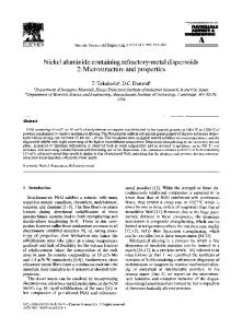
Figure 1 shows n (D) calculated for different μ values and D0 = 2 mm. The drop size distribution plays a very important role in the development of the general model because it affects both Doppler and polarization characteristics. Inertia of drops. The inertia of raindrops in a turbulent environment was estimated in Gorelik and Chernikov (1964). In the case of homogeneous and isotropic turbulence, the correlation function of turbulent wind pulsations was considered. Then the correlation function of drop velocities was derived from the solution of a linear equation for the component of drop velocity. The comparison of these two correlation functions yields the condition of obtaining an undistorted spectrum of turbulent pulsations from the drop velocities (Doppler velocities), assuming that the interaction of the drops with the medium is defined by the Stokes law. This consideration allowed Gorelik and Chernikov to derive the relaxation time T of a droplet with a given effective size D. The difficulty with this approach is the tran-

514

F. YANOVSKY

Fig. 1. Normalized gamma distribution of raindrops with D0 = 2 mm and μ = 0, 1, 2, and 3. D is given in mm.

Table 1. Relationship between raindrop diameter and relaxation time D, mm

6

5

4

3

2

1

0.5

0.1

T, s

19.8

19.5

18.8

17

14

8.65

4.38

0.538

sition from the Euler to the Lagrange scale. The relaxation time multiplied by the dimension factor Vw gives the appropriate spatial scale of turbulence. In Gorelik and Chernikov (1964), the value Vw = 10 ms – 1 was used as a typical parameter for the calculations. In the phenomenological model described below, the Vw can be changed during the adaptation. The relationship between the raindrop diameter D and its relaxation time T is summarized in Table 1 taken from Gorelik and Chernikov (1964). 3.3.2. Turbulence Scales of turbulence. The instantaneous velocity of the turbulent flow can be considered to result from the superposition of three-dimensional fluctuations and the average air motion. The turbulent velocity components follow a normal distribution with a zero mean (Dobrolensky 1969). Turbulence has an eddy nature with a wide spectrum of spatial scales L: from a minimum (inner) scale Linner up to a large (outer) scale Louter which may be comparable to the scale of the airflow as a whole. However, in our model, only the inertial subrange (Frisch 1995) of turbulence is taken into consideration. It includes all scales existing in the free atmosphere, from the smallest ones (several mm) up to about Louter (set to 1500 m). This scale range encompasses the characteristic size of the radar spatial resolution as well as the scales of turbulence dangerous for aircraft. Energy spectrum of turbulence. The turbulence energy spectrum S (Ω ) is the decomposition of the kinetic energy of turbulence in a Fourier series over wave


515

numbers Ω = 2π L (the spatial frequency). In the inertial subrange, where the conditions of homogeneity and local isotropy of turbulence are satisfied, the analytical expression for the spectrum is as follows: S (Ω ) = C ε 2 3 Ω −5 3 ,

(29)

where C is a dimensionless constant and ε is the eddy dissipation rate. The Ω is defined as Ω = | Ω | = 2π L , where Ω is the three-dimensional turbulence wave vector. The dimensionless constant C depends on the direction of the velocity vector component. The one-dimensional spectra Su, Sv, and Sw for the components u (along the basic flow) as well as v and w (across the basic flow) are also described by Eq. (29), but with different values of C. The longitudinal, Cu, and transversal, Cv and Cw, constants are related by Cv = Cw = 4Cu 3. According to experimental data (Vinnichenko et al. 1968), Cu approximately equals 0.50 with a 20% uncertainty. Taking into account that Cu ≈ 0.327C (Vinnichenko et al. 1968), we can derive Cu ≈ 0.40 − 0.60, Cv = Cw ≈ 0.53 − 0.80, and C ≈ 1.22 − 1.83. One can find different estimates of these constants in the literature, but they all have the same order of magnitude. Variance of turbulence velocity. Estimating the spatial spectrum S (Ω ) experimentally is very difficult. That is why simpler statistical parameters such as the velocity variance σ v2 are often used. The velocity variance due to turbulence in a given range of scales can be calculated from the energy spectrum S (Ω ) (Vinnichenko et al. 1968): Ω max

σ v2 =

∫ S (Ω ) dΩ ,

(30)

Ω min

where Ω min = 2π Lul and Ω max = 2π Lll correspond to the upper and lower limits of the turbulence scales considered. Substituting Eq. (29) into Eq. (30), integrating, and taking into account that the effect of Lll, which is much weaker than that of Lul, can be neglected, yields: σ v ≈ C 01 2ε 1 3 L1ul3 .

(31)

In our model, the upper scale Lul does not have to be identical to the outer scale of turbulence. Instead, it depends on the spatial resolution of the radar. Turbulence at scales much larger than the radar resolution does not affect the velocity variance, but changes the observed mean velocity. Turbulence intensity. The kinetic energy of turbulence is passed sequentially from larger scales to smaller ones and then dissipates at a scale L ≈ Linner . The latter process is quantified by the eddy dissipation rate ε , which is a fundamental parameter of turbulence characterizing its intensity. It does not depend on the scale of turbulence within the inertial subrange, which makes ε a convenient initial

516

F. YANOVSKY

Table 2. Turbulence classification based on the eddy dissipation rate ε , cm 2 s – 3

< 0.2

0.2 – 3.4

3.4 – 42.9

42.9 – 550

> 550

Intensity scale

negligible

light

moderate

heavy

severe

Fig. 2. Coordinates systems. X, Y, Z − main (radar) coordinates; XA, YA, ZA − antenna coordinates; η, ζ, ξ − particle coordinates; O – radar; ZA − antenna beam; θ − elevation; δ − particle canting angle; φ − polarization angle; and ξ − the symmetry axis of a spheroid.

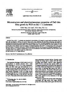
modeling parameter. The classification of turbulence from the standpoint of aircraft safety in terms of ε is shown in Table 2 (MacCready 1964). The value of ε in cumulonimbus clouds can reach 1000 cm 2 s – 3. The eddy dissipation rate ε and the spatial scale L are the only important parameters of turbulence in our model. They are used to calculate the effect of turbulence on the behavior of the particles in the radar volume. 3.3.3. Coordinates The coordinates of the mutual locations of the radar system, the moving antenna beam, and the scatterer are shown schematically in Fig. 2, in which: O is the point where the radar system is located; X, Y, and Z are the basic (radar) coordinates; ZA is the direction of the antenna beam; XA, YA, and ZA are coordinates associated with the antenna beam; θ is the antenna elevation (the angle between the OZA and XOY planes);


517

η, ζ , and ξ are the particle coordinates; δ is the particle canting angle; φ is the polarization angle; ξ is the axis of symmetry of the spheroid representing the particle.

3.4. Modeling velocity distribution of raindrops 3.4.1. Distribution of the drop fall velocity In the absence of winds, the drop fall velocity vector is directed straight down; the radar only measures the projection of this vector on the line of sight. Introducing the elevation angle θ in Eq. (22) yields v f ( D) = α − β e −0.6 D ,

(32)

where α = 9.65 sin θ and β = 10.3 sin θ . The drop fall velocity v f is assumed to be a function of the random parameter D, which obeys the known PDF as given by Eq. (28). According to Venttsel’ (1998), dividing Eq. (26) by the derivative | dvv dD | and substituting D(v f ) yields the analytical expression of the drop fall velocity distribution (Yanovsky et al. 2001):

N f (v f ) =

5 N 0 ⎛⎜ 5 β ln 3(α − v f ) ⎜⎝ 3 α − v f

μ

⎞ α − vf ⎡ ⎟ exp ⎢ 5(3.67 + μ ) ln ⎟ 3 β D 0 ⎣ ⎠

⎤ ⎥ , v f ≥ 0. ⎦

(33)

The PDF of the fall velocity can be obtained by normalization: n f (v f ) = N f ( v f )

∫N

f

(v f ) dv f .

(34)

The integration of Eq. (34) over v f can be done analytically (Yanovsky 1998a), but the resulting expressions are rather bulky and are not given here. The values of Eq. (34) for D0 =1.5 and θ = 45° are shown in Fig. 3. The calculations were done for different values of the spread parameter of the gamma size distribution: μ =1, 2, 5, 7. A significant effect of μ is obvious from these plots. The most probable fall velocity shifts to greater values when μ increases; however, the maximum velocity remains almost the same. 3.4.2. Drop turbulent velocity distribution The detection of turbulence in clouds and precipitation by a Doppler radar requires scatterers to respond instantly to the turbulent motion. However, scatterers such as raindrops may not respond perfectly due to inertia. In this section the velocity distribution of raindrops due to turbulence is calculated. Concept of a threshold turbulence scale. To make a raindrop move, a turbulent eddy must have enough energy; the larger the raindrop the more energy is needed.

518

F. YANOVSKY

Fig. 3. Radial drop fall velocity distribution for different drop size distributions and antenna elevations under the condition of constant volume of water in m3 (approximately the same rain rate); vf is given in m s – 1.

In Yanovsky (1996), a new approach was adopted to model the interaction of turbulence and raindrops with the purpose of accounting for the inertia in the simulation of the reflected signal. It was based on an earlier work by Fishman and Yanovsky (1983). In this approach, the key is the assumption that a threshold turbulent scale Lthres exists and is specific for a given mass (and size) of drops. According to this approach: • below a threshold scale, turbulent eddies do not affect raindrops of a certain size; this threshold scale Lthres corresponds to a raindrop size Dthres ; • turbulence at scales larger than the threshold scale Lthres affects all raindrops with sizes D < Dthres ; • turbulence at scales smaller than the threshold scale Lthres does not affect the raindrops with D ≥ Dthres ; • once raindrops are set into motion they act as perfect tracers of turbulence, i.e., the inertia does not play a role anymore. Thus each drop diameter Dthres corresponds to a unique value of the threshold spatial scale Lthres , i.e., Lthres and Dthres are functionally related values: Lthres = f ( Dthres ). General expression. Based on this concept, the drop turbulent velocity distribution for drops with a diameter D can be obtained as follows: Lul

pT (vT , D, ε ) =

∫ w (v T

Lthres ( D )

T

L, ε ) w ( L) dL ,

(35)


519

where wT (v T L , ε ) is the conditional probability density of turbulence velocity and w(L) is the probability density of spatial scales for given turbulence parameters. As follows from Section 3.2.2, any component of the random turbulent velocity field follows the normal distribution law with zero mean and the variance depending on the eddy dissipation rate ε and spatial scales L of turbulence according to Eq. (31):

wT (v T L , ε ) =

1 2π C0 ε 1 3 L1 3

⎛ ⎞ vT2 ⎟. exp ⎜⎜ − 23 23 ⎟ π ε C L 2 0 ⎝ ⎠

(36)

Turbulence scale distribution. Since L and ε are functionally related random variables (Venttsel’ 1998), we derive the function w(L) from w( L) =

S [Ω ( L)] , | dL dΩ |

where the PDF of the variable Ω is defined by Eq. (29) after appropriate normalization. Finally, the normalized density function w(L) can be written as follows (Yanovsky 1996): w( L) =

2 −1 3 − 2 3 L Lul . 3

(37)

Lul appears as the upper limit of integration over L and can be interpreted as the largest spatial scale of turbulence taken into account, the lower limit being set to zero.

Analytical solution. Substitution of Eqs. (36) and (37) into Eq. (35) yields: pT [vT Lthres ( D )] =

2 ε −1 3 L−ul2 3 3 πC 0

Lul

⎛ v 2ε − 2 3 L− 2 3 ⎞ ⎟ dL. L− 2 3 exp ⎜⎜ − 2π C0 ⎟⎠ ⎝ Lthres ( D )

∫

(38)

The integral in Eq. (38) can be expressed analytically in terms of the error function erf ( x ) (Venttsel’ 1998). Then the equation for pT [vT Lthres ( D )] is as follows (Yanovsky et al. 2001): pT [vT Lthres ( D)] =

[*] , 3 π 1 2 C0 L2outer ε2 3

(39)

where ⎛ ⎞ ⎛ ⎞ v2 v2 3 ⎟ [*] = 21 2 ε 1 / 3 L1ul3C01 2 exp ⎜⎜ − 2 3 2 3 ⎟⎟ − 21 2 ε 1 3 L1thres C01 2 exp ⎜⎜ − 2 3 2 3 ⎟ ⎝ 2ε Lul C0 ⎠ ⎝ 2ε LthresC0 ⎠ ⎞ ⎛ ⎞ ⎛ v v + π 1 2v erf ⎜⎜ 1 2 1 3 1 3 1 2 ⎟⎟ − π 1 2v erf ⎜⎜ 1 2 1 3 1 3 1 2 ⎟⎟ . ⎝ 2 ε LthresC0 ⎠ ⎝ 2 ε Lul C0 ⎠

520

F. YANOVSKY

Fig. 4. Partial distribution for different ε and D. Dotted curve: ε = 1 cm 2 s – 3 and D = 1 mm; solid curve: ε = 1 cm 2 s – 3 and D = 4 mm; dashed curve: ε = 100 cm2/s3 and D = 1 mm; dotdashed curve: ε = 100 cm 2 s – 3 and D = 4 mm.

Limits of integration. The lower integration limit in Eq. (35), Lthres (D), is the minimal spatial scale affecting all raindrops with equivolumetric diameters ≤ D. The numerical relationship between the diameter D and the relaxation time presented in Table 1 is used to determine Lthres (D). It can be approximated as follows: Lthres ( D ) = 21.17 ( 1 − e − 0.527 D ) Vw ,

(40)

where Vw is a constant having the dimension of velocity (ms – 1); it relates the droplet relaxation time with the scale of turbulence. Note that D and Lthres (D) in Eq. (40) are expressed in millimeters and meters, respectively. The upper integration limit Lul follows from the maximum spatial scale of turbulence contributing to random motion of scatterers in the radar volume (Yanovsky 1998b). It can be defined as the scale of turbulence that affects individual particles in a single resolution volume differently. Scales larger than Lul only influence the mean particle velocity. In fact, it is the largest characteristic size of a single resolution volume in radial or tangential direction: Lul = max( Rrad , Rtan ). Calculations. Equation (39) allows one to calculate the partial distribution of turbulence-induced velocity for raindrops of a given diameter D for the turbulence parameters C0 , Lul , and ε . Figure 4 shows the results for C0 = 1.5, Vw = 10 ms – 1, and Lul = 1000 m (Yanovsky et al. 2001). Two pairs of distributions can be seen. The pair of narrower distributions corresponds to light turbulence (ε = 1 cm 2 s – 3), while the pair of broader ones corresponds to heavy turbulence (ε = 100 cm 2 s – 3).


521

Fig. 5. Distribution of turbulent velocities of the drop ensemble.

Each pair depicts the results for two drop diameters: the upper curve corresponds to small drops (D = 1 mm), while the lower one corresponds to large drops (D = 4 mm). The integration of Eq. (39) over D yields the drop turbulent velocity distribution accounting for all the drops within the integration limits: Dmax

∫ p (v , D) N (D) dD,

N T (vT ) =

T

T

(41)

Dmin

where pT (vT, D) is defined by Eq. (38) or (39); N(D) is defined by Eq. (26); Dmin and Dmax are the bounding drop-diameter values. Figure 5 shows NT (vT) for the median drop size D0 = 1.6 mm, dispersion factor μ = 1, and three values of the eddy dissipation rate ε : 1, 10, and 100 cm 2 s – 3. The results demonstrate that the greater the eddy dissipation rate ε the broader the distribution caused by turbulence. N T (vT ) dvT is the number of raindrops in a unit volume with turbulent velocity component values between vT and vT + dvT provided that pT (vT, D) is normalized according to the following condition: ∞

∫ p (v , D) dv T

T

T

= 1.

−∞

3.4.3. Drop velocity distribution caused by both turbulence and gravity The separate velocity distributions Nf (vf ) and NT (vT) due to gravity and turbulence, respectively, were derived above. Expressing the total drop velocity as v = vf + vT and neglecting the correlation between the two components, the combined PDF can be determined by convolution. However, taking into account that the terminal fall velocity of a drop is unambiguously related to the drop diameter

522

F. YANOVSKY

Fig. 6. Radial drop velocity distribution in the Marshall – Palmer case for two values of ε and two antenna elevations θ.

according to Eq. (22), we can write the partial velocity distribution p p (v D) for a given drop by substituting vT = v − v f in Eq. (39) (Yanovsky et al. 2005). In this case the partial distribution for a given drop diameter D written in the form of a conditional distribution is as follows: p p (v D) = pT [(v − v f ) D],

(42)

where pT is given by Eq. (38) or (39). Integrating over all droplet diameters yields the distribution of radial velocities of the ensemble: Dmax

p Σ (v ) =

∫ p {[ v − v T

f

( D, θ )] D} N ( D) dD .

(43)

Dmin

After normalization, one obtains the PDF model for Doppler velocities of the drops in the resolution volume: ∞

p (v ) = p Σ (v )

∫p

Σ

(v) dv .

(44)

−∞

Figure 6 shows p(v) in the Marshall – Palmer case (μ = 0) for light (dashed curves) and heavy (solid curves) turbulence and two modes of sounding: (i) an-


523

Fig. 7. Radial drop velocity distribution for different μ (D0 = 2 mm, ε = 50 cm 2 s – 3, θ = 90°, Lul = 1000 m, and Vw = 3.5 ms – 1).

tenna is pointed towards zenith (θ = 90°) and (ii) the antenna elevation angle is 20°. The rest of the parameters are fixed: D0 = 2 mm, Lul = 350 m, and Vm = 3.5 ms – 1. It is seen that the θ = 90° curves are shifted to the right of the θ = 20° curves because the drop radial fall velocity is maximal when the antenna is pointed towards zenith. The maxima corresponding to heavy turbulence are significantly broader than those for light turbulence. The degree of broadening due to turbulence is more apparent at small elevation angles (θ = 20°) than at large elevation angles (θ = 90°). More positive velocities (relative to the radar) are seen in the case of zenith sounding, while more negative velocities occur in heavy turbulence. This figure demonstrates clearly that in the case of sufficiently strong turbulence, negative velocities appear in the convoluted velocity spectrum. These results will serve us as the basis for Doppler spectra calculations Figure 7 shows the behavior of the drop velocity distribution for different values of the dispersion factor μ of the drop size distribution. The curves become more symmetric when the parameter μ is increased. Increasing the turbulence eddy dissipation rate ε enhances the spread of the velocity distribution, as shown in Fig. 8 generated for μ = 3, D0 = 1.6 mm, θ = 30°, Lul = 1000 m, and Vw = 3.5 ms – 1. A similar effect occurs when Lul is increased, e.g., by enlarging the radar resolution cell. Finally, the parameter Vw has a rather weak effect on the resulting drop velocity distribution. Figure 9 shows the radial drop velocity PDF for different values of the antenna elevation θ while keeping other parameters constant (ε = 50 cm 2 s – 3, μ = 3, D0 = 1.6 mm, Lul = 1000 m, and Vw = 3.5 ms – 1). In the case of near-horizontal sounding (the left-hand curve), turbulence mainly contributes to the drop velocity distribution; the role of the gravitational fall velocity becomes more pronounced when the antenna points closer to the zenith.

524

F. YANOVSKY

Fig. 8. Radial drop velocity distribution for different ε.

Fig. 9. Radial drop velocity distribution for different θ.

3.5. Polarization parameter models The models developed in the previous section do not involve explicit assumptions regarding the shape of raindrops. In this section, the non-sphericity, or more specifically, the near-spheroidal shape of the particles is taken into account, thereby enabling one to model polarization parameters of the reflected signals. 3.5.1. Drop shape and orientation parameters affecting polarization In Section 3.2.1, the axial ratio ρ was introduced as a function of the axes a1 = a2 and a3 of a spheroid. Let us assume that the volume of the spheroid is


525

equal to that of a sphere with a diameter D. Then a1 ( D ) = 0.5 D [ ρ ( D )]−1 3 and a3 ( D) = a1 ρ ( D). According to De Wolf et al. (1990), the depolarization factors λ1 , λ 2 , and λ3 of the spheroid can be calculated via the following formulas: λ3 ( D) =

1 − [e( D)]2 [e( D)]2

⎡ 1 1 + e( D ) ⎤ 2 −2 −1 ln ⎢−1 + ⎥ , e = 1 − ρ , 0 < ρ < 1, (45) 2 ( ) 1 ( ) e D − e D ⎣ ⎦

λ3 ( D) =

1 + [ f ( D)]2 [ f ( D)]2

⎡ ⎤ 1 arctan f ( D)⎥ , ⎢1 − f ( D) ⎣ ⎦

λ1 ( D) =

1 − λ3 ( D ) , λ 2 ( D) = λ1 ( D). 2

f 2 = ρ −2 − 1, ρ −1 > 1,

(46) (47)

Taking into account the relative permittivity of water ε r , the shape factors of the spheroidal raindrop are as follows: Λi ( D) = [1 + λi ( D)(ε r − 1)]−1 , i = 1, 2, 3.

(48)

Thus, in the framework of the accepted model, the drop shape can be calculated for any drop equivolumetric diameter D. Let us now consider the orientation parameters affecting the polarization of the reflected signal. The particle azimuth α and canting δ angles, the antenna elevation angle θ , and the polarization angle φ can be considered parameters characterizing the mutual orientation of the particle and the sounding wave. Simple yet rather bulky formulas for the polarimetric orientation parameters Φ HH , ΦVV , and Φ HV for co-polar (HH, VV ) and cross-polar (HV ) signals were derived by Ruschenberg (1992): Φ HH = (sin δ cos α sin φ sin θ ) 2 + (sin δ sin α cos φ ) 2 1 2

+ (cos δ sin φ cos θ ) 2 − sin 2δ cos α sin 2 φ sin 2θ 1 2

(49)

1 2

− sin 2δ sin α sin 2φ cos θ + sin 2 δ sin 2α sin 2φ sin θ , ΦVV = (sin δ cos α cos φ sin θ ) 2 + (sin δ sin α sin φ ) 2 1 2

+ (cos δ cos φ cos θ ) 2 − sin 2δ cos α cos 2 φ sin 2θ 1 2

(50)

1 2

+ sin 2δ sin α sin 2φ cos θ − sin 2 δ sin 2α sin 2φ sin θ , 1 2

Φ HV = sin 2φ[(sin δ sin α ) 2 − (sin δ cos α sin θ ) 2 1 2

− cos 2 δ + sin 2δ cos α sin 2θ ] 1 2

1 2

− cos 2φ (sin 2α sin 2 δ sin θ + sin 2δ sin α cos θ ).

(51)

526

F. YANOVSKY

According to De Wolf et al. (1990) and Ruschenberg (1992), the combined parameters taking into account both the shape and the orientation of a drop are as follows: QHH ( D, δ , α, θ ) = {Λ1 ( D) + [Λ3 ( D) − Λ1 ( D)]Φ HH (δ , α, φ , θ )}2 ,

(52)

QVV [ D, δ , α, θ ] = {Λ1 ( D) + [Λ3 ( D) − Λ1 ( D)]ΦVV (δ , α, φ , θ )}2 ,

(53)

QHV ( D, δ , α, θ ) = {[Λ3 ( D) − Λ1 ( D)]Φ HV (δ , α, φ , θ )}2.

(54)

3.5.2. Radar cross section of spheroidal drops

The models of RCS calculation for raindrops with an equivolumetric diameter D in the Rayleigh approximation were considered by De Wolf et al. (1990). Using the notation introduced in Section 3.2, the RCS of a spheroidal drop with a relative permittivity ε r at a wavelength λ >> D is given by σ xy ( D) =

π 5D6 | ε r − 1|2 Qxy , x, y = h, v. 9λ4

(55)

Here, the complex parameter Qxy = Fxy ( Λ )Φ xy (δ , α ,θ )

(56)

is responsible for the polarization characteristics of the RCS. In Eq. (56), Fxy represents the particle shape (parameterized with a vector of shape parameters Λ ) according to Eqs. (56)−(58) and (45)−(47), while Φ xy takes into account the particle orientation (parameterized by the canting angle δ and azimuth angle α) and the radar elevation angle θ according to Eqs. (49)−(51). In the special case of a spherical particle, QHH = QVV = 9 | 2 + ε r |−2 and QHV = QVH = 0, and so σ HH = σ VV = π 5 D 6 λ−4 | ε r − 1|2 | ε r + 2 |−2 and σ HV = σ VH = 0, that is, Eq. (55) is reduced to the well-known result of Rayleigh scattering. 3.5.3. Polarization parameters of an ensemble of drops

In order to calculate the conventional polarization parameters of the signal reflected from an ensemble of drops located inside the resolution volume, the integration over all scatterers must be performed. Let us calculate the polarization parameters Zdr and Ldr assuming that pδ (δ ) is the PDF of the particle canting angle, the particle azimuth α is a fixed, and N (D) is the drop size distribution: δ max Dmax

Zdr = 10 log

∫ ∫σ

HH

( D, δ , α , θ ) N ( D, D0 , μ ) pδ (δ ) dD dδ

δ min Dmin δ max Dmax

∫ ∫σ

δ min Dmin

, VV


(57)


527

Fig. 10. Zdr and Ldr [dB] as functions of D0 for different antenna elevations θ. δ max Dmax

Ldr = 10 log

∫ ∫σ

HV


δ min Dmin δ max Dmax

∫ ∫σ

. HH

(58)


δ min Dmin

An example of Zdr and Ldr calculations as functions of the median equivolumetric drop diameter D0 using the Gaussian pδ (δ ) (see Section 3.3.1) for σ δ = 30°, μ = 0, Dmin = 0.1, Dmax = 8, δ min = 0, δ max = π , and different antenna elevation angles θ is given in Fig. 10. These dependencies are consistent with common sense and actual measurements. However, owing to the integration over D they cannot be used for modeling Doppler–polarimetric spectral functions such as sZdr (v). For the purpose of Doppler polarimetry, it is not sufficient to obtain the polarization parameters as functions of an integral drop size distribution parameter such as D0. The general concept of our model (Section 3.2) requires the polarization parameters as functions of the drop diameter taking into account statistical characteristics of particle orientations. 3.5.4. Averaging over particle orientations

General expressions for the orientation-averaged parameters Qxy , H , V , described by Eq. (56) are as follows: Qxy ( D, θ ) =

∫∫Q

xy ( D, δ , α , θ ) pα (α ) pδ

(δ ) dα dδ ,

x, y =

(59)

δ α

where pα (α ) is the drop azimuth distribution and pδ (δ ) is the drop canting distribution. The polarization angle φ in the initial expressions of Qxy can be assumed to be zero without loss of generality. The expressions (52)–(54) with nonaveraged values Φ xy , x, y = H , V , can be considered as sums of squares. There-

528

F. YANOVSKY

2 2 fore, the average values of orientation parameters Φ HH , Φ HH , ΦVV , ΦVV , and 2 Φ HV are needed; they were obtained analytically by Yanovsky (1998a). For example, some simple final expressions obtained are as follows:

1 4

Φ HH ≈ [1 − exp(−2σ δ2 )],

2 Φ HH =

3 2 (e −8σ δ 64

2

− 4e − 2σ δ + 3),

1 4

ΦVV ≈ [cos 2 θ + 3 cos 2 θ exp(−2σ δ2 ) − exp(−2σ δ2 ) + 1].

(60) (61)

One can see from the expressions (60) that there is no dependence on the antenna elevation in the case of the HH polarization. Physically, this is because the plane of polarization rotates around the H polarization axis when the elevation angle is changed. 3.5.5. Polarization parameters versus equivolumetric diameter in an ensemble of drops

The average shape– orientation parameters can be derived by combining the expressions (59) with Eqs. (52)– (54) as well as the average orientation parameters i , i = 1, 2 : Φ xy 2 QHH ( D, θ , σ δ ) = Λ21 + 2Λ1 (Λ3 − Λ 1 ) Φ HH + (Λ3 − Λ 1 ) 2 Φ HH ,

(62)

2 QVV ( D, θ , σ δ ) = Λ21 + 2Λ 1 (Λ3 − Λ1 ) ΦVV + (Λ3 − Λ 1 ) 2 ΦVV ,

(63)

2 QHV ( D, θ , σ δ ) = (Λ3 − Λ 1 ) 2 Φ HV .

(64)

Because no averaging over D is performed, it is not necessary to multiply QHH, QVV, and QHV by the radar cross section σ xy (D). Finally, the differential radar reflectivity and linear depolarization ratio can be calculated as functions of D via the following formulas: Zdr = 10 log

QHH ( D, σ δ ) , QVV ( D, θ , σ δ )

Ldr = 10 log

QHV ( D, θ , σ δ ) . QVV ( D, θ , σ δ )

(65)

These expressions yield quite realistic curves of Zdr and Ldr versus D for different θ and σ δ (Yanovsky 1998a). 3.6. Doppler–polarimetric characteristics Doppler–polarimetric spectra and Doppler–polarimetric parameters such as the spectral differential reflectivity introduced theoretically in Section 2 are considered here in more detail for the case of rain. 3.6.1. Polarimetric Doppler spectra

In accordance with our main concept (Section 3.2), in the frequency domain the complex model provides Doppler spectra for different combinations of polari-


529

Fig. 11. Generalized structure of the phenomenological model developed for the computation of Doppler spectra under different conditions.

zations for transmitted and received waves. Figure 11 shows the general structure of the model, which uses as input data the parameters of the drop size distribution (DSD; μ and D0 ), the antenna elevation (θ ), the polarization mode, the parameters of turbulence (ε and L), and the radar performance specifications (not shown). Based on the mathematical models described above, the model yields the drop fall velocity distribution (DFVD); drop turbulence velocity distribution (DTVD); and RCS for a given polarization mode, DSD, particle shape, antenna elevation, wavelength, etc. Finally, the requisite spectra and Doppler–polarimetric parameters are computed (Yanovsky 2002). In the case of the HV linear polarization basis, at least three functions, S HH (v), SVV (v), and S HV (v), are generated for given conditions. They are the models of Doppler energy spectra for different combinations of polarizations of transmitted and received waves, i.e., the Doppler–polarimetric spectra: Dmax

S xy (v) =

∫ p (v D , ε , θ ) σ

xy ( D

θ , ε ) N ( D D0 ) dD, x, y = H , V .

(66)

Dmin

An example of calculations for the same hypothetic rain event but for different polarizations is shown in Fig. 12 (left-hand panel). The upper curve corresponds to the HH spectrum, while the lower curve represents the VV case. In the case of a slant sounding of rain, the horizontal polarization provides more energy in the reflected signal due to predominantly horizontal orientation of the larger axes of spheroidal drops. In the absence of turbulence, the Doppler spectrum S xyf (v) is controlled only by the DFVD and is given by S xyf (v ) dv = N f (v) σ xy (v) dv,

while including turbulence yields:

(67)

530

F. YANOVSKY

Fig. 12. Generated Doppler spectra for horizontal and vertical polarizations (left-hand panel). Three sZdr (v) curves are computed for different turbulence intensities (negligible, light, and moderate) corresponding to eddy dissipation rates ε = 0.1, 1, and 10 mm 2 s – 3 as well as for two modes of the model (right-hand panel). ∞

S xyfT

(v ) =

∫S

f xy (v − vT

) N T (vT ) d vT ,

(68)

−∞

where xy denotes the polarization pair HH, HV, or VV, and σ xy (v) is the RCS of the particle with velocity v. Since turbulence produces different wind velocities at different locations in the radar volume, equal-sized raindrops will not appear in the same velocity bin of the Doppler spectrum. This trivial aspect is important when Doppler spectra are calculated for different polarizations, as will be shown later. 3.6.2. Polarization parameters of rain as functions of the Doppler velocity

Following the Doppler–polarimetric approach, one can construct different polarimetric characteristics, for example, those corresponding to Eqs. (13) −(16), but as functions of the Doppler velocity by using the elements of the spectral target covariance matrix (19) instead of the conventional covariance matrix (12). Using the models (66) according to the above discussion, one can calculate the radar observables (20), (21), etc. for different conditions. An example of calculating the spectral differential reflectivity in rain as a function of the Doppler velocity for different turbulence intensities ε and fixed remaining parameters is shown in Fig. 12 (left-hand panel). It is seen that the sZdr(v) curve flattens with increasing intensity of turbulence. In the case of negligible turbulence (ε = 0.1 cm 2 s – 3), the larger droplets are more oblate and fall faster than the smaller ones. If scatterers become more oblate then sZdr increases. This behavior changes in the case of substantial turbulence. Because of the turbulence-induced random mixing, particles with different shapes and velocities are mixed, resulting in a flattened sZdr (v) curve. In theory, the spectral linear depolarization ratio sLdr (v) behaves similarly; however, its values in rain are rather small, typically – 30 dB and even much smaller. Obviously, it is difficult to measure such values reliably.


531

Fig. 13. Definition of the slope of the sZdr (v) curve, SLP, as the tangent of the angle α.

3.6.3. Slope of sZdr(v)

Unlike the traditional Zdr parameter (13), the sZdr (v) (20) is a function (generally nonlinear) that in the case of a rain increases monotonously. To characterize a sZdr (v) curve, the slope of sZdr (SLP) was introduced (Yanovsky et al. 2005). The SLP is estimated as the slope ratio of the tangent at the inflection point, as explained in Fig. 13. The SLP is not the only parameter analyzed previously; another informative parameter is DELTA defined as the difference between the maximum and minimum of the sZdr (v) curve (Yanovsky et al. 2003a). However, the SLP is more sensitive to turbulence intensity. 3.6.4. Differential Doppler velocity

Another Doppler– polarimetric parameter is DDV defined as the difference between the mean Doppler velocities for horizontal and vertical polarizations: ΔV = V HH − VVV (Yanovsky et al. 2003b). It can be calculated using modeled Doppler spectra according to Dmax

ΔV =

∫

v S HH (v) dv −

Dmin

Dmax

∫ vS

VV

(v) dv.

(69)

Dmin

The actual DDV varies with elevation angle θ ; this pronounced dependence can be used to retrieve useful information by comparing measurement and model results. 4. Analysis of polarimetric parameters

In this section we consider analysis results based on computing Doppler–polarimetric parameters for different conditions with the help of the phenomenological complex model described above.

532

F. YANOVSKY

Fig. 14. Relationships between the Doppler-spectrum width σ v and the sZdr (v) slope, SLP, and the intensity of turbulence in rain defined by the eddy dissipation rate ε .

4.1. Relation of SLP and slope of sZdr (v) to turbulence intensity In the practice of radar meteorology, the main parameter traditionally used to retrieve information on turbulence intensity characterized by the eddy dissipation rate ε is the Doppler spectrum width σ v (Doviak and Zrnić 1993). Figure 14 shows the relationship between σ v (ε ) and SLP (ε ) computed on the basis of mathematical models and the computer realization of the complex phenomenological model. Figure 15 confirms the strong influence of turbulence on the behavior of the spectral differential reflectivity (left-hand panel) and the spectral linear depolarization ratio. These plots are calculated for eddy dissipation rates ε ranging from 0.1 up to 100 cm 2 s – 3, which implies a wide range of turbulence intensity from negligible to severe. Figure 16 shows the effect of the drop size distribution on the relationships between SLP and other parameters. More specifically, the left-hand panel depicts SPL as a function of ε for different values of the spread parameter μ of the gamma drop size distribution, while the right-hand panel shows the inverse value 1/SLP versus the Doppler spectrum width for the same μ . 4.2. Relation of DDV to turbulence intensity and rain microstructure The first study of DDV as a radar parameter for characterizing the microstructure of weather formation was performed by Wilson et al. (1997). Their paper contains a detailed analysis of the relationship between DDV and the hydrometeor size distributions under the assumption that turbulence does not affect the former. The effect of turbulence was taken into account by Yanovsky et al. (2003b). Figure 17 shows the relation of DDV for an antenna elevation of 45° to parameters of the drop size distribution for three values of turbulence intensity: ε = 0.1 cm2 s –3


533

Fig. 15. Spectral differential reflectivity (left-hand panel) and spectral linear depolarization ratio as functions of the Doppler velocity computed for different intensities of turbulence represented by a wide range of eddy dissipation rates ε from 0.1 up to 100 cm 2 s – 3.

Fig. 16. Relationships between SLP and ε (left-hand panel) and between 1/SLP and Doppler spectrum width for different spread parameters μ of the gamma drop size distribution.

(solid curve), ε = 10 (dotted curve), and ε = 100 (dashed curve). These results show a pronounced dependence of DDV on μ and D0. It is seen that the solid and dotted curves are close to each other on both panels, which implies that light turbulence does not affect the relationships significantly. However strong turbulence (dashed curves) is rather important. The direct dependence of DDV on the eddy dissipation rate is illustrated in Fig. 18 corresponding to θ = 30°, D0 = 1.5 mm, and μ = 5. One can see that the rate of change of the function DDV = f (ε ) is increasing with ε and then is almost constant for strong and severe turbulence.

534

F. YANOVSKY

Fig. 17. Dependence of DDV on the parameters of the drop size distribution (μ and D0) for three values of the turbulence intensity ε = 0.1 cm 2 s – 3 (solid curve), ε = 10 (dotted curve), and ε = 100 (dashed curve). The antenna elevation is 45°.

Fig. 18. Dependence of DDV on the eddy dissipation rate for θ = 30°, D0 = 1.5 mm, and μ = 5.

Additional analyses of the DDV parameter and its relation to other radar parameters and the object features have been presented by Glushko and Yanovsky (2009, 2010) and Yanovsky and Glushko (2010). 5. Measurements

The Doppler–polarimetric measurements with the radar TARA (Yanovsky et al. 1997; Heijnen et al. 2000) were used for the verification of the model described above. The combination of Doppler and polarimetric measurements is discussed in Unal and Moisseev (2004). Using the measured time series of scattering matrices, we perform the Fourier transforms (or Doppler processing) and calculate the second moments of the resulting spectral scattering matrices, which yields polarimetric spectrographs. Some results were discussed in Yanovsky et al. (2005, 2007).


535

Fig. 19. Comparison of different measures of turbulence.

Measurements were performed with different antenna elevations, including vertical (zenith) sounding, but mostly in the slant sounding mode (45° and 30°). In this chapter we will not discuss the details of signal processing, but it is useful to mention that the received signal was subjected to the procedures of unfolding, clipping, averaging, and smoothing. Moments and other parameters of the Doppler spectra were estimated as well as polarimetric parameters such as sZdr (v), SLP, DDV, etc. The turbulence eddy dissipation rate was retrieved from the Doppler spectrum width using the established methodology (Doviak and Zrnić 1993) and making the correction for the drop fall velocity variance as described in Yanovsky et al. (2005). 5.1. Comparison of different parameters Comparison of different measures of turbulence is presented in Fig. 19. One can identify the maxima of all parameters, except for SLP (Slope sZdr), occurring at ~1140 m; these maxima are perfectly collocated with the SLP minimum. Space and time distributions of different Doppler–polarimetric parameters are shown in Fig. 20. The horizontal axis is time and the vertical axis is height, while the value of each parameter is shown by color according to the color bar on the right-hand side of the respective panel. All fields were obtained by processing the same raw data of light overcast rain in The Netherlands (Yanovsky et al. 2003a, 2005). One can clearly see correlation between all these parameters. For example, small (blue) values of SLP (the stripe at the ~800 m altitude) correspond to large values of the Doppler spectrum width, the eddy dissipation rate, and the rms Doppler velocity. The behavior of DDV is similar to that of SLP, but it is less sensitive

536

F. YANOVSKY

Fig. 20. Comparison of space – time behavior of Doppler – polarimetric parameters.


537

Fig. 21. Comparison of modeled and measured data.

to the turbulence intensity. The measurements show that the above-mentioned correlation is observed not only in the space domain but also in time. 5.2. Comparison between the model and measurements As an example, in Fig. 21 the model results are shown together with the processed measurements. The former are represented by triangles connected by the dashed curve. The solid gray curve shows the best lest-squares fit. We processed a ~15-min measurement dataset accumulated for overcast rain. The key parameters of the model were chosen to maximally correspond to the parameters of the real event. Specifically, D0 = 1.023 mm is the average median drop diameter retrieved from the reflectivity and rain rate; Lul = 15 m is equal to the radar resolution; θ = 45° is equal to the antenna elevation. The remaining parameters of the model were derived from the best fit to the measured data. One can see that the model is in a rather good agreement with the measurements and not too far from the best-fit curve. 6. Discussion and applications

So far the model results and the Doppler–polarimetric measurements (reflectivity, Doppler spectrum, spectral differential reflectivity, DDV, SLP) have shown

538

F. YANOVSKY

Fig. 22. Combination of modeling and measurements.

consistency, thereby implying that the model can be used to estimate the microphysics of rain events. Several comparisons have been done for light stratiform rains, in which case it is necessary to consider medium or large rain intensity in order to verify the significant differentiation in the sZdr slope with the eddy dissipation rate. For light rain rates (see Fig. 18, where D0 is ~1 mm), the sensitivity of the sZdr curve to the eddy dissipation rate is weak when the turbulence starts to be moderate (eddy dissipation rates >3 cm 2 s – 3). With this example of measurements, we cover only the interval [0, 3] ms – 1 of radial drop velocities in Fig. 15, which is not sufficient to obtain significantly different sZdr slopes. From 5 ms – 1, there is a clear differentiation of the sZdr slope when the eddy dissipation rate varies. We need, therefore, moderate to high rain intensities for a further verification and to study whether the retrieval of the eddy dissipation rate from the sZdr slope is feasible. As follows from Fig. 21, the combination of modeling and measurements makes it possible to obtain much indirect information about the object of observation, specifically, on the microstructure of and turbulence in rain. The mathematical representation of the object described above and the relations between its components and the radar sounding waveform improve our understanding and allow the inference of the microstructure and turbulence properties of rain by comparing modeled and measured data and tuning the model to bring its results in agreement with the object. This is illustrated in Fig. 22. The approach developed can be used operationally to improve the quality of radar meteorological information. New parameters SLP, DDV, and other polarimetric characteristics are independent of the Doppler spectrum width and other conventional parameters and, therefore, can be used together to obtain more reliable and comprehensive information on the microstructure and turbulence of rain as well as for the retrieval of the hydrometeor type.


539

7. Conclusions

The Doppler–polarimetric radar is a powerful tool for remote sensing of rain. The potential of Doppler polarimetry exceeds significantly that of the sum of the Doppler technique and polarimetry used separately. Doppler– polarimetric techniques provide promising capabilities for data interpretation. However, the number of variables grows significantly and the mutual interrelations between them are rather complicated. The interpretation of Doppler–polarimetric measurements requires an adequate model capable of relating the Doppler–polarimetric observables to the parameters of precipitation. Such a model has been created and described in this chapter. The approach presented has facilitated the selection of certain Doppler– polarimetric parameters helping to retrieve turbulence parameters in precipitation as well as the microstructure of rain. The results of actual data processing using different approaches have demonstrated good agreement. The application of independent turbulence-related variables can improve the reliability and accuracy of radar retrievals in rain. Measurements of weather-related objects by Doppler–polarimetric radars can be very useful in solving the wave propagation problem for the tasks of microwave remote sensing, communications, and radar detection of targets embedded in intensely cluttered backgrounds. The continued research in this field should result in further improvements of models, the development of algorithms and devices for real-time measurements, more efficient processing, coverage of objects other than rain, optimal combination of different parameters, and adaptive methods of measurements and signal processing. Our approach to the Doppler–polarimetric modeling is promising, deserves further development, and may play an important role in radar remote-sensing data interpretation and signal processing. Acknowledgments

The project on Doppler polarimetry was supported in part by STW (the Dutch Technology Foundation). It was part of a joint project of the International Research Centre for Telecommunications and Radar (IRCTR) at TU-Delft and the National Aviation University in Kyiv. The author is grateful to H. Russchenberg, C. Unal, L. Ligthart, A. Yarovoy, O. Krasnov, and S. Heijnen for cooperation during collaborative work in TU-Delft. References Atlas, D., R. C. Srivastava, R. S. Sekhon, 1973: Doppler radar characteristics of precipitation at vertical incidence. Rev. Geophys. Space Phys. 11, 1–35. Bachmann, S., and D. S. Zrnić, 2006: Spectral density of polarimetric variables separating biological scatterers in the VAD display. J. Atmos. Oceanic Technol. 24, 1186−1198.

540

F. YANOVSKY

Beard, K. H., and C. Chuang, 1987: A new model for equilibrium shape of rain drops. J. Atmos. Sci. 44, 1509−1524. Bringi, V. N., and V. Chandrasekar, 2001: Polarimetric Doppler Weather Radar: Principles and Applications (Cambridge University Press, Cambridge, UK). Brussaard, G., 1976: A meteorological model for rain-induced cross polarization. IEEE Trans. Antennas Propag. 24, 5−11. De Wolf, D. A., H. W. J. Russchenberg, and L. P. Ligthart, 1990: Effective permittivity of and scattering from wet snow and ice droplets at weather radar wavelengths. IEEE Trans. Antennas Propag. 38, 1317−1325. Dobrolensky, Yu. P., 1969: Dynamics of Flight in Turbulent Atmosphere (Transport Press, Moscow) (in Russian). Doviak, R. J., and D. S. Zrnić, 1993: Doppler Radar and Weather Observations (Academic Press, San Diego). Fishman, B. E., and F. J. Yanovsky, 1983: To the theory of radar signals’ formation reflected from meteorological objects. Radiotekhnika, 56−57 (in Russian). Frisch, U., 1995: Turbulence: The Legacy of A. N. Kolmogorov (Cambridge University Press, Cambridge, UK). Foote, G. B., and P. S. du Toit, 1969: Terminal velocity of rain drops aloft. J. Appl. Meteorol. 8, 249–253. Glushko, D. N., and F. J. Yanovsky, 2009: DDV – novel Doppler – polarimetric technique for remote sensing of precipitation. In Proceedings of the 6th European Radar Conference (Rome), pp. 298−301. Glushko, D. N., and F. J. Yanovsky, 2010: Analysis of differential Doppler velocity for remote sensing of clouds and precipitation with dual-polarization S-band radar. J. Microwave Wireless Technol. 2, 391−398. Gorelik, A. G., and A. A. Chernikov, 1964: Some results of the radar investigation of the wind structure on heights 50 − 700 m. Trudy (Proc.) Central Aerological Observ. 57, 3−17 (in Russian). Heijnen, S. H., L. P Ligthart, and H. W. J. Russchenberg, 2000: First measurements with TARA; an S-Band transportable atmospheric radar. Phys. Chem. Earth. B 25, 995−998. Kezys, V., E. Torlaschi, and S. Haykin, 1993: Potential capabilities of coherent dual polarization X-band radar. In Proceedings of the 26th International Conference on Radar Meteorology (American Meteorological Society, Boston), pp. 106–108. Kozlov, A. I., L. P. Ligthart, and A. I. Logvin, 2002: Mathematical and Physical Modelling of Microwave Scattering and Polarimetric Remote Sensing (Kluwer, Dordrecht). Kubesh, R. J., and K. V. Beard, 1993: Laboratory measurements of spontaneous oscillations for moderate-size raindrops. J. Atmos. Sci. 50, 1089−1098. Kwiatkowski, J. M., A. B. Kostinski, and A. R. Jameson, 1995: The use of optimal polarizations for studying the microphysics of precipitation: nonattenuating wavelengths. J. Atmos. Oceanic Technol. 12, 96–114. Ligthart, L. P., and L. R. Nieuwkerk, 1980: FM-CW Delft atmospheric research radar. Proc. IEE F 127, 421−426. MacCready, P., 1964: Standardization of gustiness values from aircraft. J. Appl. Meteorol. 3, 439−449. Pruppacher, H. R., and K. V. Beard, 1970: A wind tunnel investigation of the internal circulation and shape of water drops falling at terminal velocity in air. Quart. J. R. Meteorol. Soc. 96, 247–256. Pruppacher, H. R., and J. D. Klett, 1997: Microphysics of Clouds and Precipitation (Kluwer, Dordrecht).


541

Pruppacher, H. R., and R. L. Pitter, 1971: A semi-empirical determination of the shape of cloud and rain drops. J. Atmos. Sci. 28, 86−94. Rogers, R. R., 1990: The early years of Doppler radar in meteorology. In D. Atlas, Ed., Radar in Meteorology (American Meteorological Society, Boston), pp. 122−129. Russchenberg, H. W. J., 1992: Ground-based remote sensing of precipitation using a multipolarized FM-CW Doppler radar. PhD Thesis (Delft University, Delft). Russchenberg, H. W. J., 1994: Combined radar measurements of the Doppler spectrum and the linear depolarization ratio of rain: a turbulence-canting model. In Proceedings of the 3rd International Symposium on Tropospheric Profiling (Hamburg), pp. 456−459. Ryzhkov, A. V., 2001: Interpretation of polarimetric radar covariance matrix for meteorological scatterers: theoretical analysis. J. Atmos. Oceanic Technol. 18, 315−328. Seliga, T. A., and V. N. Bringi, 1976: Potential use of radar differential reflectivity measurements at orthogonal polarizations for measuring precipitation. J. Appl. Meteorol. 15, 69–76. Seliga, T. A., R. G. Humphries, and J. I. Metcalf, 1990: Polarization diversity in radar meteorology: early developments. In D. Atlas, Ed., Radar in Meteorology (American Meteorological Society, Boston), pp. 109−114. Shupiatsky, A. B., 1959: Radar scattering by non-spherical particles. Trudy (Proc.) Central Aerological Observ. 30, 39−52 (in Russian). Tokay, A., and K. V. Beard, 1996: A field study of raindrop oscillations. Part I: Observation of size spectra and evaluation of oscillation causes. J. Appl. Meteorol. 35, 1671− 1687. Unal, C. M. H., D. N. Moisseev, F. J. Yanovsky, and H. W. J. Russchenberg, 2001: Radar Doppler polarimetry applied to precipitation measurements: introduction of the spectral differential reflectivity. In Proceedings of the 30th International Conference on Radar Meteorology (American Meteorological Society, Boston), pp. 316–318. Unal, C. M. H., and D. N. Moisseev, 2004: Combined Doppler and polarimetric radar measurements: correction for spectrum aliasing and nonsimultaneous polarimetric measurements. J. Atmos. Oceanic Technol. 21, 443–456. Venttsel’, E. S., 1998: Probability Theory (Vysshaya Shkola, Moscow) (in Russian). Vinnichenko, N. K., N. Z. Pinus, C. M. Shmeter, and G. N. Shur, 1968: Turbulence in Free Atmosphere (Gidrometeoizdat, Leningrad) (in Russian). Wilson, R., A. J. Illingworth, and T. M. Blackman, 1997: Differential Doppler velocity: a radar parameter for characterizing hydrometeor size distributions. J. Appl. Meteorol. 36, 649–663. Yadong, W., X. Xiao, and T.-Y. Yu, 2008: Spectral analysis of dual-polarization radar signals in a tornadic supercell storm. In Proceedings of the 24th Conference on Severe Local Storms (Savannah, GA), pp. 1–10. Yanovsky, F. J., 1996: Simulation study of 10 GHz radar backscattering from clouds and solution of the inverse problem of atmospheric turbulence measurements. Comput. Electromagn. IEE CP 420, 188–193. Yanovsky, F. J., 1998a: Model of the relationship between Doppler and polarization parameters of the radar signal from precipitation. Report No. IRCTR-S-002-98 (Technical University, Delft). Yanovsky, F. J., 1998b: Simulation of the processes of interaction between radar signal and turbulized meteorological object. Visnyk KMUTSA 1, 125–136 (in Ukrainian). Yanovsky, F. J., 2002: Phenomenological models of Doppler – polarimetric microwave re-

542

F. YANOVSKY

mote sensing of clouds and precipitation. IEEE Int. Geosci. Remote Sens. Symp. IGARSS-02, Vol. 3, pp. 1905–1907. Yanovsky, F. J., and D. N. Glushko, 2010: Simulation study of relationships between Doppler polarimetric parameters at microwave remote sensing of precipitation. In Proceedings of the 7th European Radar Conference (Paris), pp. 148–151. Yanovsky, F. J., and L. P. Ligthart, 2000: Microwave remote sensing of dangerous meteorological phenomena. In Proceedings of the XIII International Conference on Microwave, Radar and Wireless Communications, Vol. 3, pp. 70–82. Yanovsky, F. J., L. P. Ligthart, and H. W. J. Russchenberg, 1997: Analysis of transportable atmospheric radar (TARA) possibilities for the remote sensing of dangerous meteorological phenomena. In PIERS (Cambridge, MA), p. 116. Yanovsky, F. J., H. W. J. Russchenberg, and L. P. Ligthart, 2001: Doppler – polarimetric models of microwave remote sensing of rain. In Proceedings of the 11th Conference on Microwave Technique (University of Pardubice, The Czech Republic), pp. 47–62. Yanovsky, F. J., C. M. H. Unal, and H. W. J. Russchenberg, 2003a: Doppler – polarimetric radar measurements of turbulence in rain. Report IRCTR-S-006-03 (Technical University, Delft). Yanovsky, F. J., C. M. H. Unal, and H. W. J. Russchenberg, 2003b: Relationship between differential Doppler velocity and turbulence intensity in rain: modeling and measurements. In Proceedings of the 6th International Symposium on Tropospheric Profiling (Leipzig), pp. 306–308. Yanovsky, F. J., H. W. J. Russchenberg, and C. M. H. Unal, 2005: Retrieval of information about turbulence in rain by using Doppler – polarimetric radar. IEEE Trans. Microwave Theory Tech. 53, 444–450. Yanovsky, F. J., C. M. H. Unal, H. W. J. Russchenberg, and L. P. Ligthart, 2007: Doppler – polarimetric weather radar: returns from wide spread precipitation. Telecommun. Radio Eng. 66, 715–727. Zrnić, D., and D. Boren, 2008: Weather radar – recent developments and trends. In Proceedings of the Microwaves, Radar and Remote Sensing Symposium (Kiev), pp. 174– 179.

From left to right: Adrian Doicu, Sergey Savenkov, and Felix Yanovsky.

Inferring microstructure and turbulence properties in rain ... - CiteSeerX

Inferring microstructure and turbulence properties in rain ... - CiteSeerX

Suggest Documents

Microstructure, mechanical and functional properties of ... - CiteSeerX

Microstructure and properties of nanocrystalline copper - CiteSeerX

Microstructure and mechanical properties of Polypropylene - CiteSeerX

Rain-induced turbulence and air-sea gas transfer - CiteSeerX

Microstructure and properties

MICROSTRUCTURE AND MECHANICAL PROPERTIES

Microstructure and Mechanical Properties

Relationship between Microstructure and Mechanical Properties in ...

Microstructure, Mechanical Properties and in vitro

Microstructure and Mechanical Properties in Progressively Drawn ...

Microstructure and superconducting properties in air ...

Inferring low-dimensional microstructure representations using ...

Inferring Atmospheric Turbulence Structure Using Synthetic Aperture ...

linking meteorology, turbulence, and air chemistry in the amazon rain

Microstructure, soft magnetic properties and

Microstructure and photoluminescence properties of

Rheological properties and microstructure ...

Material properties and microstructure from

MICROSTRUCTURE AND MECHANICAL PROPERTIES OF ...

MICROSTRUCTURE AND MECHANICAL PROPERTIES OF ...

Microstructure, optical properties, and catalytic

Material properties and microstructure from

rock elastic properties: dependence on microstructure - CiteSeerX

improved accuracy in inferring the fine scale properties of rain rate