Infinite Petri Nets: Part 1, Modeling Square Grid Structures - Wolfram

Infinite Petri Nets: Part 1, Modeling Square Grid Structures Dmitry A. Zaitsev

Vistula University Warsaw, Poland Ivan D. Zaitsev

Ershov Institute of Informatics Systems Novosibirsk, Russia Tatiana R. Shmeleva

National Academy of Telecommunications Odessa, Ukraine A composition and analysis technique was developed for investigation of infinite Petri nets with regular structure, introduced for modeling networks, clusters and computing grids, that also concerns cellular automata and biological systems. A case study of a square grid structure composition and analysis is presented. Parametric description of Petri nets, parametric representation of infinite systems for the calculation of place/transition invariants, and solving them in parametric form allowed the invariance proof for infinite Petri net models. Complex deadlocks were disclosed and a possibility of network blocking via ill-intentioned traffic revealed.

1. Introduction

Grid computations [1, 2] allow considerable extending of the tasks that are solvable in a reasonable time; that in some cases is the crucial point for new technology development. The cost of supercomputing is extremely high, which makes the cost of errors high as well, both in protocols and in their hardware and software implementations. Reallife grid computing is closely connected with numerical methods of solving systems of differential and integral equations in sophisticated application areas such as weather forecasting and nuclear physics. A Petri net is a bipartite directed graph with a dynamic process defined on it [3]. One part of the vertices is named places and drawn as circles; another part of the vertices is named transitions and drawn as bars (rectangles). Arcs could be multiple, and their multiplicity is represented by integer numbers. Dynamic elements are named tokens and drawn as dots; they are situated inside places and move within the net. https://doi.org/10.25088/ComplexSystems.26.2.157

158

D. A. Zaitsev, I. D. Zaitsev and T. R. Shmeleva

Petri nets [3, 4], which were successfully applied for verification of telecommunication protocols [5–8], are a prospective formalism for grid analysis. Petri nets and their extensions [9, 10] find wide application in manifold other domains [11–15]. As far as the results are appreciated in the form applicable for grids of any size, for their verification infinite Petri nets with regular structure were introduced for the first time by the authors of the present paper. The progress is indicated by the dimension and form of the studied structures: linear, treelike, square and hypercube [16–18]. In the mentioned works, the only edge condition studied, except open edges, was the attachment of plug devices, which could be considered as a primitive model of some terminal device (computer). As real-life grid computing is closely connected with numerical methods, on some surface for flat grids, various realistic edge conditions were investigated as well [8]; for instance, closing the edges of a rectangle gives a torus surface. The present paper is focused on the analysis of square grid models via the technique of proving p-invariance, because p-invariant Petri nets are structurally conservative and bounded, which are the properties of ideal systems models. Moreover, other forms of grids on planes and in space are considered. The most significant result is obtained for a hypercube structure of arbitrary size with an arbitrary number of dimensions. The presented results are supplied with software generators of Petri net models of grid structures, and models of grids of a given size are constructed in an automated way to acknowledge the obtained results and gain a series of results for inductive conclusions on grid properties. However, at the present stage of research it is rather difficult to obtain a generalized technique of composition for infinite Petri nets with regular structure [19] similar to [20]. Recently, infinite Petri nets have found wide application for modeling cellular automata [21] and representing a canvas of cell connections in a generalized neighborhood [22] that spans the range between von Neumann’s and Moore’s neighborhoods; software generators of the canvas are available on github.com/dazeorgacm/hmn. All the models presented in the paper were constructed and analyzed in the system TINA [23], supplied with plug-ins Deborah and Adrian [16], and are available for free download on the website of the first author, member.acm.org/~daze.

2. Basic Notions and Definitions

A Petri net is a bipartite directed graph on which a discrete dynamic process is defined. The first part of the vertices, named places, is depicted by circles; the second part of the vertices, named transitions, Complex Systems, 26 © 2017

Infinite Petri Nets: Part 1, Modeling Square Grid Structures

159

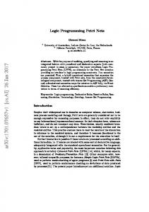
is depicted by bars (rectangles); dynamic elements, named tokens, are depicted by dots situated inside places. Tokens are consumed and produced by transitions as result of their firing. A transition is fireable if each input place contains at least a token. The behavior of a net is a step-by-step process; on each step, an arbitrary fireable transition fires. When firing, a transition consumes a token from each input place and puts a token into each output place. In Figure 1, an example of the transition firing is shown, along with a graph of reachable markings (GRM) of a Petri net, which is a complete formal description of its behavior. In the general case, GRM is infinite, which requires developing special methods of Petri net analysis.

(a)

( b)

(c) Figure 1. Behavior of a Petri net: (a) initial marking; (b) next marking;

(c)�GRM.

A Petri net occupies a unique position within the hierarchy of discrete systems: it is more powerful than a finite automaton and less powerful than a Turing machine. Thus, it provides instruments of the system’s behavior specification inaccessible in the formalism of finite automata. In addition, a series of the system’s properties analysis tasks are decidable problems, in contrast to Turing machines. As basic Petri net properties, boundedness, conservativeness and liveness are considered. A bounded Petri net has a finite GRM; conservativeness consists in preserving a weighted sum of tokens; in a live Petri net, each transition can fire in a trace starting from any reachable marking. There are two basic approaches to analysis of finite Petri nets: the first based on state-space analysis using graphs of reachable and coverable markings; the second based on the state equation and invariants. Moreover, there are two basic auxiliary techniques: reduction— decreasing Petri net size while preserving its properties, and decomposition—dividing the Petri net into parts of certain forms. https://doi.org/10.25088/ComplexSystems.26.2.157

160


Matrix methods of Petri net analysis are based on application of the Petri net state equation (Murata equation) Δμ  C · σ, where Δμ is a difference of the initial and final markings, C is the incidence matrix of a Petri net and σ is a vector that counts firings of transitions. Integer non-negative solutions x (y) of homogeneous system x · C  0 (C · y  0) are named invariants of places or p-invariants (of transitions or t-invariants). An invariant Petri net, having an invariant with all natural components, is a bounded and conservative net under any initial marking; moreover, a transition’s firing sequence could be constructed so that it leads to the initial marking.

3. Composition of Clans

Components, used for composition of infinite structures, are functional subnets (clans) of Petri nets [16], which have been well studied when investigating the usual (finite) models, for instance, in the process of protocol TCP verification. Input places of a clan have only outgoing arcs and output places only incoming arcs. The composition of a protocol TCP model from its clans is represented in Figure 2.

(a)

Complex Systems, 26 © 2017


161

(b) Figure 2. Composition of protocol TCP model: (a) clans of protocol TCP

model; (b) model of protocol TCP.

Compositional analysis [16] allowed speedup of the verification processes of complex networking protocols because of solving a sequence of linear systems built on the net topology, with lesser dimension, which is essential when finding solutions in the non-negative domain (monoid) for Diophantine systems (ring).

4. Linear Infinite Structure

Marsan’s model [24] of a workstation for the Ehernet network with common bus architecture (Figure 3(a)) requires composition of an a priori indefinite number of devices for complete verification of technology, but not a definite given net. An example of a bus with four devices is represented in Figure 3(b). In [16], the task of computing linear invariants for the Marsan model was solved via calculation of the clans’ invariants and their composition in parametric form for obtaining a parametric solution. As a parameter of the linear structure, the number of workstations on a bus was used. As far as the final solution possesses definite properties for any natural value of the parameter, it is convenient to name the general approach an investigation of infinite Petri nets with regular structure.

https://doi.org/10.25088/ComplexSystems.26.2.157

162


(a)

(b) Figure 3. Models of the Ethernet network with common bus architecture:

(a) workstation; (b) network with four workstations.

Regularity of structure consists in the fact that a single component (clan) was used and the rules of composition of the model from a linear sequence of components were defined based on the operation of fusion (union) of contact places of neighboring clans. Afterward, methods were developed for components that are subnets with contact places of general form (without subdivision into input and output), as well as providing usage of a few different components. The structure of the component’s connections is given by a graph, either directed for clans or undirected in the general case when abstracting from the directions of arcs.

5. A Generalized Model of a Communication Device

Communication devices of the packet-switching networks, such as switches and routers, consist of a finite number of ports and implement the forwarding of the arrived (from a port) packet to the destinaComplex Systems, 26 © 2017


163

tion port. Packet header information and a switch/router address table are used for the calculation of the destination port number. The device implements either the compulsory buffering of packets into its internal buffer or cut-through possibilities. Even cut-through devices employ buffering when the destination port is busy. Ports work in fullduplex mode, providing two channels for receiving and sending packets; moreover, ports have their own buffers for each channel with the capacity available for the storing of, usually, one packet. In the present paper, we abstract from packet headers and address tables and consider devices with compulsory buffering only. All the capacities are measured in the number of packets. Computer networks are built via connection of communication and terminal devices; as communication devices, either active or passive equipment is used; switches and routers are the basic active equipment. The generalized model of a communication device takes into consideration such peculiarities of the packet-switching network’s functioning as the full-duplex mode of work, forwarding packets among ports and buffering with limited capacity of buffers. An example of a communication device model with four ports, which is used later for composition of the rectangular grid, is represented in Figure 4. Because the model was constructed in the TINA system, which does not provide subscript symbols, an index is written as a suffix after the underscore character “_” in TeX-like notation. For instance, ti1,3 looks like {ti_1,3}. An internal buffer of a device is represented by the five following central places: pbl, limitation of the buffer capacity; pb1 , pb2 , pb3 , pb4 , sections of the buffer for storing packets redirected to ports 1, 2, 3, 4, respectively. Models of each port are the same and represented by four places and four transitions. For instance, places pi1 , pil1 of the first port model the input buffer of the port and limitation of its capacity, respectively; places po1 , pol1 model the output buffer of the port and limitation of its capacity, respectively. The port output channel is modeled by transition to1 , which extracts a packet from the section of the internal buffer pb1 and inserts a packet into the port buffer po1 ; in addition to that, the available space of the internal buffer pbl is incremented by unit and the available space of the port buffer pol1 is decremented by unit. The port input channel is modeled by three alternative transitions ti1,2 , ti1,3 , ti1,4 , which define the possible variants of the packet switching; from the input port buffer pi1 a packet is forwarded into one of the internal buffer sections, pb2 , pb3 or pb4 . The buffer sizes are measured in the number of packets; the port buffer sizes are chosen equal to unit, which is in accord with the majority of real-life devices. https://doi.org/10.25088/ComplexSystems.26.2.157


164

Figure 4. Model of a communication device with four ports.

In the subsequent composition of models, both in this paper and in Part 2, forthcoming, the number of the device’s ports varies; that is why it is reasonable to represent the model in the following parametric form with a parameter np equal to the number of ports. A Petri net specification via enumerating its transitions is convenient; note that for a connected Petri net, it provides the enumeration of all its places as well: tou : pbu , polu → pou , pbl tiu,v : piu , pbl → pbv , pilu , v  1, np, v ≠ u

, u  1, np .

(1)

A row of a transition description has the form t : pi , … , pi → pj , … , pj , where the transition name is written 1

x

1

y

before a semicolon symbol: on the left of the symbol “→”, its input places are listed, and on the right, its output places. The loop-like notation u  1, np means using integer values sequentially in the specified range from 1 to np. Application of indexing and aggregation of rows allow the description of sets of transitions. So for instance, the Complex Systems, 26 © 2017


165

first row of the expression in equation (1) describes np transitions and the second row describes np · np - 1 transitions. The parametric description allows the representation of infinite systems of equations for calculating Petri net invariants. Besides, it is possible to construct a dual parametric description that enumerates the places of a Petri net; such a parametric description is convenient for calculation of the transition’s invariants.

6. A Rectangular Infinite Structure

Let us consider the composition of an open rectangular communication grid. Devices’ models with this form, shown in Figure 5, are situated in the cells of a rectangular matrix and are indexed using two upper indices; a square matrix of size k > 0 was chosen. Neighboring devices are connected via fusion (union) of contact places; places are situated in the order, shown in Figure 4, that provides connection of the output port channel of a device with the input port channel of a neighboring device and vice versa. Thus, a device Ri, j , 0 < i < k, 0 < j < k is connected to the following neighbors: Ri, j-1 to the left, Ri, j+1 to the right, Ri-1, j to the top and Ri+1, j to the bottom, in such

Figure 5. Composition of an open rectangular grid.


166


a way that port 1 is connected to port 3 of the upper device and port�4 is connected to port 2 of the left device. As a result of this composition, fusion places have duplicate notation with respect to each of the �neighbor devices. For instance, places poi,1 j , poli,1 j , pii,1 j , pili,1 j of j j j j the device Ri, j coincide with places pii-1, , pili-1, , poi-1, , poli-1, 3 3 3 3 of the device Ri-1, j , respectively. For unambiguous notation of contact places, the indices of the left port 4 and upper port 1 are used; as a result, the pending contact places of the right and bottom edges of the grid contain index k + 1 of nonexistent neighbor devices. An example of a grid of size 2⨯2 is represented in Figure 6.

Figure 6. Composition of the open square grid model of size 2 ⨯ 2.

The parametric description of the obtained grid has the following form. Each port is described with two rows; the first row corresponds to the port output channel and describes a single transition of the current device; the second row corresponds to the port input channel and describes three transitions of the current device indexed via internal parameter v: Complex Systems, 26 © 2017


167

i, j toi,1 j : poli,1 j , pbi,1 j → poi,j 1 , pbl , i, j i, j → pili, j , pbi, j , tii,j 1, v : pi1 , pbl 1 v v  2, 3, 4, j j toi,3 j : pili+1, , pbi,3 j → pii+1, , pbli, j , 1 1 i+1, j j , pbli, j → poli+1, , pbi,v j , tii,j 3, v : po1 1 v  1, 2, 4,

toi,4 j : poli,4 j , pbi,4 j → poi,4 j , pbli, j ,

, i  1, k, j  1, k .

(2)

tii,4,jv : pii,4 j , pbli, j → pili,4 j , pbi,v j , v  1, 2, 3, toi,2 j : pili,4 j+1 , pbi,2 j → pii,4 j+1 , pbli, j , tii,2,jv : poi,4 j+1 , pbli, j → poli,4 j+1 , pbi,v j , v  1, 3, 4 In the rows 1, 2 and 5, 6, corresponding to ports 1 and 4, the contact places of the current device Ri, j are written. In the rows 3, 4 and 7, 8, corresponding to ports 2 and 3, the contact places of a neighboring device are written: for port 2 to port 4 of the neighboring to the right device, Ri, j+1 ; for port 3 to port 1 of the neighboring to the bottom device, Ri+1, j . Moreover, the port channel is altered to the opposite: the input i to the output o and the output o to the input i, which corresponds to the grid composition rules. The parameter of the description in equation (2) is the size of the square grid k; to represent a rectangular grid, two parameters could be considered as well. The open square grid structure of size k is denoted as Sk . In Figure 3 and others showing the models obtained via the system TINA and software generators, the notation of the net element’s names avoids subscript and superscript symbols; the grid node index is written as a suffix in TeX-like notation: the lower index after the underscore character “_” and the upper index after the hat character 7 “^”. For instance, ti5, 1, 3 looks like {ti_1,3^5,7}.

7. Edge Conditions

The built grid model could be employed for the design of commutation matrices of networking devices, investigation of computer grids and supercomputers devised for solving boundary value problems of big size and other application domains. The model of an open grid in Figure 6 is a base for constructing https://doi.org/10.25088/ComplexSystems.26.2.157


168

definite closed models. The following varieties of the edge conditions of the grid’s models were studied: ◼ terminal (customer) device, Figure 7 ◼ truncated communication device, Figure 8 ◼ connection of (opposite) edges, Figure 9

7.1 A Grid with Terminal Device on Edges

The communication devices may be attached to each other, constituting a communication structure, but they are created only for packet transmission among the terminal devices: workstations and servers. In this paper, the client-server technique of interconnection is not studied, so the types of terminal devices are not distinguished. An abstract terminal device provides at least two basic functions: send packet and receive packet. These basic functions are provided by the models represented in Figure 7. To stress the difference between terminal and communication devices’ elements, different symbols are used to denote places and transitions of the terminal device models: symbol q for places and symbol s for transitions.

(a)

( b)

Figure 7. Models of a terminal device: (a) simple reflection of packets;

(b) with the packet’s buffering.

Figure 7(a) gives the simplest model that only reflects the arrived packets from the input to the output via transition s; names of the places are given with respect to the places of a communication device port. So the model of a terminal device may be attached by the fusion of the places with the same names. The model in Figure 7(b) contains an internal buffer of the packets qb; transition si models the input of the packets, while transition so models the output. To distinguish terminal devices attached to the upper, right, bottom and left edges, the lower index with the numbers 1, 2, 3 and 4 of the corresponding port is used; for instance, s21 means transition of the terminal device of the upper edge (port 1) attached to the device R1, 2 . An example of the communication matrix with attached terminal devices (type a) is represented in Figure 8(a).



169

(a)

(b) Figure 8. An example of the rectangular grid with specific edge conditions:

(a) with attached terminal devices on the edges; (b) with truncated devices on edges.


170


Simple models of terminal devices (Figure 7) could be developed in more detail when investigating the computational aspects of grid functioning, and supplied by subnets modeling the processes of solving the task. The obtained parametric description of the square grid with terminal device of type Figure 7(a) has the following form: toi,1 j : poli,1 j , pbi,1 j → poi,1 j , pbli, j , tii,1,jv : pii,1 j , pbli, j → pili,1 j , pbi,v j , v  1, 4, v ≠ 1, j j toi,3 j : pili+1, , pbi,3 j → pii+1, , pbli, j , 1 1 j j tii,3,jv : poi+1, , pbli, j → poli+1, , pbi,v j , 1 1

v  1, 4, v ≠ 3, toi,4 j : poli,4 j , pbi,4 j → poi,4 j , pbli, j , tii,4,jv : pii,4 j , pbli, j → pili,4 j , pbi,v j , v  1, 4, v ≠ 4,

, i  1, k, j  1, k .

(3)

toi,2 j : pili,4 j+1 , pbi,2 j → pii,4 j+1 , pbli, j , tii,2,jv : poi,4 j+1 , pbli, j → poli,4 j+1 , pbi,v j , v  1, 4, v ≠ 2, j 1, j 1, j 1, j sj1 : po1, 1 , pil1 → pi1 , pol1 , j j j j sj3 : pik+1, , polk+1, → pok+1, , pilk+1, , 1 1 1 1

si4 : poi,4 1 , pili,4 1 → pii,4 1 , poli,4 1 , si2 : pii,4 k+1 , poli,4 k+1 → poi,4 k+1 , pili,4 k+1  Comparing the parametric description of the open grid in equation�(2), four rows were appended to the end, describing transitions of attached terminal devices in the following order: sj1 (upper-edge devices), sj3 (bottom-edge devices), si4 (left-edge devices) and si2 (rightedge devices). Upper and left terminal devices use contact places of the neighbor communication device, while bottom and right terminal devices use their own contact places according to the composition agreements. The square grid structure of size k with attached terminal devices is denoted as STk .



171

7.2 Grid with Truncated Communication Devices on Edges

Truncated devices on edges (Figure 8(b)) is the most realistic variety of model for the grid nodes combining packet switching with packet processing. Edge ports are truncated together with other Petri net vertices that suppose usage of absent ports. Thus, eight types of boundary devices appear, which are shown in Figure 8(b) on the grid example of size 3⨯ 3. The concept of the truncated device consists in removing all the pendent ports on the edges of the grid, including their contact places, incidental transitions and the corresponding partitions of the internal buffer. Thus, while removing port u of the current device, all the places and transitions with index u are removed. An example for a square grid of size 3 is shown in Figure 8(b), where only the central device coincides with Figure 4 and edge devices are truncated: two ports are removed for corner devices and one port for the rest of the edge devices. There are eight types of truncated devices Ri, j depending on their location: left (j  1, i ≠ 1, i ≠ k)—without port 4; left-upper (i  1, j  1)—without ports 4, 1; upper (i  1, j ≠ 1, j ≠ k)—without port 1; right-upper (i  1, j  k)—without ports 1, 2; right (j  k, i ≠ 1, i ≠ k)—without port 2; right-bottom (i  k, j  k)—without ports 2, 3; bottom (i  k, j ≠ 1, j ≠ k)—without port 3; left-bottom (i  k, j  1)—without ports 3, 4. For the composition of the square grid in the following, the same parametric description of the device in equation (1) at np  4 is used; the Petri net model is named SUk . The edge ports are truncated, including all their places and transitions via additional limitations for indices of definite ports: i ≠ 1 for port 1, i ≠ k for port 3, j ≠ 1 for port 4, j ≠ k for port 2. Moreover, some input transitions tii,u,jv are truncated for v, equaling absent ports; corresponding transitions are present at: i > 1 for v  1, j < k for v  2, i < k for v  3, j > 1 for v  4:


172


toi,1 j : poli,1 j , pbi,1 j → poi,1 j , pbli, j , i ≠ 1, tii,1,j2 : pii,1 j , pbli, j → pili,1 j , pbi,2 j , i ≠ 1, j < k, tii,1,j3 : pii,1 j , pbli, j → pili,1 j , pbi,3 j , i ≠ 1, i < k, tii,1,j4 : pii,1 j , pbli, j → pili,1 j , pbi,4 j , i ≠ 1, j > 1, j j toi,3 j : pili+1, , pbi,3 j → pii+1, , pbli, j , 1 1 i ≠ k, j j tii,3,j1 : poi+1, , pbli, j → poli+1, , pbi,1 j , 1 1 i ≠ k, i > 1, j j tii,3,j2 : poi+1, , pbli, j → poli+1, , pbi,2 j , 1 1 i ≠ k, j < k, j j tii,3,j4 : poi+1, , pbli, j → poli+1, , pbi,4 j , 1 1 i ≠ k, j > 1,

toi,4 j : poli,4 j , pbi,4 j → poi,4 j , pbli, j , j ≠ 1, tii,4,j1 : pii,4 j , pbli, j → pili,4 j , pbi,1 j , j ≠ 1, i > 1, tii,4,j2 : pii,4 j , pbli, j → pili,4 j , pbi,2 j , j ≠ 1, j < k, tii,4,j3 : pii,4 j , pbli, j → pili,4 j , pbi,3 j , j ≠ 1, i < k, toi,2 j : pili,4 j+1 , pbi,2 j → pii,4 j+1 , pbli, j , j ≠ k, tii,2,j1 : poi,4 j+1 , pbli, j → poli,4 j+1 , pbi,1 j , j ≠ k, i > 1, tii,2,j3 : poi,4 j+1 , pbli, j → poli,4 j+1 , pbi,3 j , j ≠ k, i < k, tii,2,j4 : poi,4 j+1 , pbli, j → poli,4 j+1 , pbi,4 j , j ≠ k, j > 1


, i  1, k, j  1, k .

(4)


173

The grid composition uses the names of the left and upper ports (4 and 1) only; that is why contact places with port numbers 2 and 3 do not appear in equation (4). For instance, the transitions of the third port are described as j j , pbi,3 j → pii+1, , pbli, j toi,3 j : pili+1, 1 1

instead of the obvious toi,3 j : poli,3 j , pbi,3 j → poi,3 j , pbli, j . The square grid structure of size k with truncated communication devices is denoted as SUk . 7.3 A Grid with Connected Opposite Edges (Torus)

Connection of the grid edges allows us to obtain various surfaces, frequently used for solving practical tasks. For instance, the opposite edges connection of the open rectangular grid (Figure 9) leads to obtaining a torus widely applied in nuclear physics.

(a)

(b)

(c)

Figure 9. Connection of opposite edges: (a) open grid; (b) connection of edges

1, 3; (c) connection of edges 2, 4.

The parametric description of the grid is represented by the following and named SCk :



174

toi,1 j : poli,1 j , pbi,1 j → poi,1 j , pbli, j , tii,1,jv : pii,1 j , pbli, j → pili,1 j , pbi,v j , v  1, 4, v ≠ 1, j j toi,3 j : pili+1, , pbi,3 j → pii+1, , pbli, j , 1 1 i ≠ k, j j , pbli, j → poli+1, , pbi,v j , tii,3,jv : poi+1, 1 1

i ≠ k, v  1, 4, v ≠ 3, toi,4 j : poli,4 j , pbi,4 j → poi,4 j , pbli, j , tii,4,jv : pii,4 j , pbli, j → pili,4 j , pbi,v j , v  1, 4, v ≠ 4, toi,2 j : pili,4 j+1 , pbi,2 j → pii,4 j+1 , pbli, j , j ≠ k,

, i  1, k, j  1, k .

(5)

tii,2,jv : poi,4 j+1 , pbli, j → poli,4 j+1 , pbi,v j , j ≠ k, v  1, 4, v ≠ 2, j 1, j k, j 1, j k, j tok, 3 : pil1 , pb3 - > pi1 , pbl , j 1, j k, j → pol1, j , pbk, j , tik, 3, v : po1 , pbl 1 v

v  1, 4, v ≠ 3, toi,2 k : pili,4 1 , pbi,2 k → pii,4 1 , pbli, k , tii,2,kv : poi,4 1 , pbli, k → poli,4 1 , pbi,v k , v  1, 4, v ≠ 2 Comparing to equation (2), descriptions for ports of the right and bottom edges (i  k, j  k) are separated at the foot of equation (4), and corresponding transitions use contact places of the opposite edge (i  1, j  1). For instance, on the right edge instead of toi,2 j : pili,4 j+1 , pbi,2 j → pii,4 j+1 , pbli, j the description toi,2 k : pili,4 1 , pbi,2 k → pii,4 1 , pbli, k is used. Note that, comparing to equation (3), all the input transitions tii,u,jv of the same port u are grouped in a single line (because separate truncating conditions are not required) and the parameter v  1, 4 is added.



175

The square grid structure of size k with connected opposite edges is denoted as SCk .

8. An Infinite System of Equations and Dual Parametric Description

The matrix form x · C  0 of the system representation for the places invariants calculation is inconvenient for the infinite systems construction. Sometimes in the literature, the structure of matrix C is considered and simple rules of the system equation’s composition are formulated: an equation is constructed for each transition and represents an equality of sums for input and output places of a transition. Applying this rule to the parametric description of the grid Sk in equation (2), we obtain this infinite system equation: toi,1 j : -xpoli,1 j - xpbi,1 j + xpoi,1 j + xpbli, j  0, tii,1,jv : -xpii,1 j - xpbli, j + xpili,1 j + xpbi,v j  0, v  2, 3, 4, j j toi,3 j : -xpili+1, - xpbi,3 j + xpii+1, + xpbli, j  0, 1 1 j j tii,3,jv : -xpoi+1, - xpbli, j + xpoli+1, + xpbi,v j  0, 1 1 v  1, 2, 4,

toi,4 j : -xpoli,4 j - xpbi,4 j + xpoi,4 j + xpbli, j  0,

(6)

tii,4,jv : -xpii,4 j - xpbli, j + xpili,4 j + xpbi,v j  0, v  1, 2, 3, toi,2 j : -xpili,4 j+1 - xpbi,2 j + xpii,4 j+1 + pbli, j  0, tii,2,jv : -xpoi,4 j+1 - xpbli, j + xpoli,4 j+1 + xpbi,v j  0, v  1, 3, 4 ; i  1, k, j  1, k. It is required to find a solution for an arbitrary natural value of the parameter k that allows calling the system infinite. It is supposed that a finite parametric specification of the solution will be obtained that contains the parameter k. The system is a Diophantine one; that is, it contains integer values of coefficients; moreover, it is required to find its solutions in the monoid of non-negative integer numbers. For the present time, universal methods of solving such systems are unknown. A system of equations (6) for calculation of the place invariants is composed directly on the parametric description of the grid. Construction of analogous systems for the transition invariants requires application of a dual parametric description of the grid, because an equation is constructed for each place and represents an equality of sums for input and output transitions of a place. The (direct) parametric description of infinite Petri nets with regular structure developed and successfully applied in Sections 4–6 conhttps://doi.org/10.25088/ComplexSystems.26.2.157


176

sists of lines with the following form: ti : pinj * apinj , … → poutj * apoutj , …; indices_range, k

k

l

l

where ti is the described transition, pinj its input places, poutj its outk

l

put places and apinj , apoutj denotes the multiplicity of correspondk

l

ing arcs; multiplicity equal to unit is omitted. Thus, for the ordinary Petri net, the following notation is used: ti : pinj , … → poutj , … ; indices_range. k

l

The direct parametric description is very useful for composition of infinite systems of linear algebraic equations of the form of equation�(6) for calculating p-invariants of infinite Petri nets with regular structure. The equation of the system constructed on it has the form -xpinj · apinj - ⋯ + xpoutj · apoutj + ⋯  0; indices_range, k

k

l

where xpinj , xpoutj k

l

l

are unknowns corresponding to Petri net

places. But the direct parametric description does not help much at calculating t-invariants of infinite Petri nets with regular structure because in the system for calculating t-invariants, equations correspond to places and unknowns correspond to transitions. And constructing such a system on the direct parametric description is not a trivial task. That is why other methods were applied for calculating t-invariants that are based on explicitly constructing cyclic transitions firing sequences. Let us introduce the dual parametric description of infinite Petri nets with regular structure that consists of lines with the following form: pj : tini * atini , … → touti * atouti , …; indices_range, k

k

l

l

where pj is the described place, tini its input transitions, touti its k

l

output transitions, and atini , atouti denotes the multiplicity of correk

l

sponding arcs; multiplicity equal to unit is omitted. Thus, for the ordinary Petri net, the following notation is used: pj : tini , … → touti , …; indices_range. k

l

To calculate t-invariants, closed grids should be studied, since the open models are not consistent. The simplest closed model ST1 is obtained via attaching terminal devices shown in Figure 7(a) to the sides of the internal device shown in Figure 4. Attached edge transitions are named su , where index u equals the number of the internal device port. The dual parametric description of a closed node ST1 has the following form: Complex Systems, 26 © 2017


177

(pou : tou → su ), polu : su → tou , piu : su → tiu, v , v  1, 4, v ≠ u,

, u  1, 4

pilu : tiu, v , v  1, 4, v ≠ u → su ,

.

(7)

pbu : tiu, v , v  1, 4, v ≠ u → tou  pbl : tou , u  1, 4 → tii,u,jv , v  1, 4, v ≠ u, u  1, 4 A problem arises regarding the duplicate naming of contact places that are merged in the process of grid composition. In Section 4, the problem was solved using the names of upper and left ports only (number 1 and 4, respectively). The same solution is used here. For j is written, and instance, instead of using pii,3 j , the place name poi-1, 1 instead of using pii,2 j , the place name poi,4 j-1 is written; it is the case for internal devices of grid only with the indices i > 1, j > 1. So the edge devices should be described separately. Note that devices on the bottom and right borders of the grid use indices of nonexistent devices with the value k + 1, since only the names of ports 4 and 1 are considered. The dual parametric description of the closed square grid in equation (3) has the form represented further part-by-part for clearness. 1. The open grid nodes without the upper row and left column: j poi,1 j : toi,1 j → tii3,-1, v , v  1, 4, v ≠ 3, i,j j poli,1 j : tii3,-1, v , v  1, 4, v ≠ 3 → to1 ,

pii,1 j : toi3-1, j → tii,1,jv , v  1, 4, v ≠ 1, pili,1 j : tii,1,jv , v  1, 4, v ≠ 1 → toi3-1, j , poi,4 j : toi,4 j → tii,2,jv-1 , v  1, 4, v ≠ 2, poli,4 j : tii,2,jv-1 , v  1, 4, v ≠ 2 → toi,4 j , , i  2, k, j  2, k .

(8)

pii,4 j : toi,2 j-1 → tii,4,jv , v  1, 4, v ≠ 4, pili,4 j : tii,4,jv , v  1, 4, v ≠ 4 → toi,2 j-1 , pbi,u j : tii,u,jv , v  1, 4, v ≠ u → toi,u j ,

u  1, 4, pbli, j : toi,u j , u  1, 4 → tii,u,jv , v  1, 4, v ≠ u, u  1, 4



178

The sequel of expressions is constructed on equation (8) having some peculiarities: with different values of indices i, j; with different transitions of neighboring node on one or two ports; without internal part contained in some other expression. 2. The upper border nodes and terminal devices: poi,1 j : toi,1 j → sj1 , poli,1 j : sj1 → toi,1 j , pii,1 j : sj1 → tii,1,jv , v  1, 4, v ≠ 1, pili,1 j : tii,1,jv , v  1, 4, v ≠ 1 → sj1 , poi,4 j : toi,4 j → tii,2,jv-1 , v  1, 4, v ≠ 2, poli,4 j : tii,2,jv-1 , v  1, 4, v ≠ 2 → toi,4 j ,

, i  1, j  2, k .

(9)

pii,4 j : toi,2 j-1 → tii,4,jv , v  1, 4, v ≠ 4, pili,4 j : tii,4,jv , v  1, 4, v ≠ 4 → toi,2 j-1 , pbi,u j : tii,u,jv , v  1, 4, v ≠ u → toi,u j ,


3. The left border nodes and terminal devices: j poi,1 j : toi,1 j → tii3,-1, v , v  1, 4, v ≠ 3, i, j j poli,1 j : tii3,-1, v , v  1, 4, v ≠ 3 → to1 ,

pii,1 j : toi3-1, j → tii,1,jv , v  1, 4, v ≠ 1, pili,1 j : tii,1,jv , v  1, 4, v ≠ 1 → toi3-1, j , poi,4 j : toi,4 j → si4 , poli,4 j : si4 → toi,4 j , pii,4 j : si4 → tii,4,jv , v  1, 4, v ≠ 4, pili,4 j : tii,4,jv , v  1, 4, v ≠ 4 → si4 , pbi,u j : tii,u,jv , v  1, 4, v ≠ u → toi,u j ,



, i  2, k, j  1 .

(10)


179

4. The upper-left corner node and terminal devices: poi,1 j : toi,1 j → sj1 , poli,1 j : sj1 → toi,1 j , pii,1 j : sj1 → tii,1,jv , v  1, 4, v ≠ 1, pili,1 j : tii,1,jv , v  1, 4, v ≠ 1 → sj1 , poi,4 j : toi,4 j → si4 , poli,4 j : si4 → toi,4 j ,

, i  1, j  1 .

pii,4 j : si4 → tii,4,jv , v  1, 4, v ≠ 4,

(11)

pili,4 j : tii,4,jv , v  1, 4, v ≠ 4 → si4 , pbi,u j : tii,u,jv , v  1, 4, v ≠ u → toi,u j ,


5. The bottom border terminal devices: j poi,1 j : sj3 → tii3,-1, v , v  1, 4, v ≠ 3, j j poli,1 j : tii3,-1, v , v  1, 4, v ≠ 3 → s3 ,

pii,1 j : toi3-1, j → sj3 ,

, i  k + 1, j  1, k .

(12)

, i  1, k, j  k + 1 .

(13)

pili,1 j : sj3 → toi3-1, j ,

6. The right border terminal devices: poi,4 j : si2 → tii,2,jv-1 , v  1, 4, v ≠ 2, poli,4 j : tii,2,jv-1 , v  1, 4, v ≠ 2 → si2 , pii,4 j : toi,2 j-1 → si2 , pili,4 j : si2 → toi,2 j-1 ,

Parametric description equations (8)–(13) could be aggregated in the united one-piece description and even condensed using additional internal parameters, but it makes the representation form more sophisticated. Parametric systems for calculating t-invariants of Petri nets are composed easily on their dual parametric description. As an equation corresponds to a place and states the balance of arcs connecting it with its input and output transitions, the equation constructed on (2) has the form -ytini · atini - ⋯ + ytouti · atouti + ⋯  0; indices_range. k

k

l

l



180

The unknowns are traditionally named y, with the suffix corresponding to the name of a transition. The system composed on the dual parametric description equation (7) of ST1 has the following form: -ytou + ysu  0 -ysu + ytou  0 -ysu +



ytiu, v  0

v1,4,v≠u

. , u  1, 4 -



ytiu, v + ysu  0

.

(14)

v1,4,v≠u

-



ytiu, v + ytou  0

v1,4,v≠u

-  ytou + u1,4



ytiu, v  0

u1,4,v1,4,v≠u

This system contains a finite number of equations. But when composing a system on the parametric descriptions, a system is obtained with the number of equations depending on the value of the parameter k.

9. Analysis of Infinite Nets

For the present time, three groups of research methods were developed for investigating infinite Petri nets with regular structure: ◼ via solving infinite systems of linear Diophantine equations in non-nega-

tive integer numbers for calculation of Petri net invariants ◼ via explicit construction of cyclic transitions firing sequences ◼ via auxiliary graphs of packets transmission and possible blockings of

devices 9.1 Solving Infinite Systems of Equations

For finding Petri net invariants, infinite homogeneous systems of linear Diophantine equations (6) are applied, which should be solved in non-negative integer numbers. A heuristic ad hoc technique was devel-



181

oped to compose the parametric solutions. Then, it is strictly proven that the parametric specification describes solutions of equation (6). Composition of solutions and proofs is done individually for each variety of grid. 9.1.1 Open Grid

The universal methods for solving the infinite systems of the linear equations under the rings (integer numbers), especially into semigroups (non-negative integer numbers), are unknown. We applied a heuristic method of a general solution construction in the parametric form. The general solution of equation (6) for grid Sk may be represented as: pii,1 j , pili,1 j , i  1, k + 1, j  1, k; poi,1 j , poli,1 j , i  1, k + 1, j  1, k; pii,4 j , pili,4 j , i  1, k, j  1, k + 1; poi,4 j , poli,4 j , i  1, k, j  1, k + 1; pbi,1 j , pbi,2 j , pbi,3 j , pbi,4 j , pbli, j , i  1, k, j  1, k; pili,1 j , poli,1 j , pili,4 j , poli,4 j , pbli, j , i  1, k, j  1, k;,

.

(15)

j pili,4 k+1 , poli.k+1 , i  1, k, pilk+1, , polk+1.j , j  1, k 1 1 4

pii,1 j , poi,1 j , pii,4 j , poi,4 j , pbi,u j , u  1, 4;, i  1, k, j  1, k;, j , i  1, k, pik+1, , pok+1.j , j  1, k pii,4 k+1 , poi.k+1 1 1 4

The way the solutions are described is common enough for sparse vectors and especially for the Petri net theory. Only nonzero components are mentioned by the name of a corresponding place. The nonzero multiplier 1 is omitted; in case it is not the unit, the notation p * x is used, where x is the value of the invariant for place p. Such notation is adopted in the TINA software, which was used for obtaining the Petri net figures in this paper. A line of the matrix in equation�(15) gives us a set of lines according to the indices i and j, except the last two lines, which contain a variable number of components given by indices. The total number of solutions is  5 · k2 + 4 · k + 2. Npinv k We did not manage to prove that equation (15) is the basis of nonzero solutions of equation (6), but it is possible to prove that each



182

line of equation (15) is a solution of equation (6). And this fact allows the proof of p-invariance for the net Sk . Lemma 1.

Each line of the matrix in equation (15) is a solution of equa-

tion (6). Proof. Let us substitute each parametric line of equation (15) into each parametric equality of equation (6). This gives us the correct statement. For instance, let us substitute the first line of equation (15) ′

′

′

′

pii1 , j , pili1 , j , i′  1, k, j′  1, k + 1 into the second equality of equation (6) xpii,1 j + xpbli, j  xpili,1 j + xpbi,2 j , i  1, k, j  1, k. We obtain: ◼ When i′ ≠ i or j′ ≠ j: 0 + 0  0 + 0 and further 0  0. ◼ When i′  i and j′  j: 1 + 0  1 + 0 and further 1  1.

In the same way, all the 16⨯7 combinations may be checked. □ Theorem 1.

The net Sk is a p-invariant Petri net for an arbitrary natural

number k. Proof. Let us consider the sum of the sixth and seventh lines of equation (15), which represents the solutions of equation (6) according to Lemma 1: pii,1 j , poi,1 j , pii,4 j , poi,4 j , pbi,1 j , pbi,2 j , pbi,3 j , pbi,4 j , i  1, k, j  1, k, j j pii,4 k+1 , poi,4 k+1 , i  1, k, pik+1, , pok+1, , j  1, k 1 1

plus pili,1 j , poli,1 j , pili,4 j , poli,4 j , pbli, j , i  1, k, j  1, k, j j pili,4 k+1 , poli,4 k+1 , i  1, k, pilk+1, , polk+1, , j  1, k 1 1

equals pii,1 j , pili,1 j , poi,1 j , poli,1 j , pii,4 j , pili,4 j , poi,4 j , poli,4 j , pbi,1 j , pbi,2 j , pbi,3 j , pbi,4 j , pbli, j , i  1, k, j  1, k, pii,4 k+1 , pili,4 k+1 , poi,4 k+1 , poli,4 k+1 , i  1, k, j j j j pik+1, , pilk+1, , pok+1, , polk+1, , j  1, k. 1 1 1 1


(16)


183

As all the Npk  13 · k2 + 8 · k places are mentioned in this invariant, the Petri net Sk is a p-invariant net for an arbitrary natural number k. Moreover, as each component of equation (16) equals the unit, the net Sk is a conservative and bounded Petri net for an arbitrary natural number k. □ As the p-invariance was proven for an arbitrary natural number k, we say that the invariants of infinite Petri nets with the regular structure were studied. The proof that equation (15) is a basis of equation (6) solutions is appreciated. But this fact was only substantiated by the calculation experiments for the sequence k  1, … , 10. Solutions given by equation (15) were compared with the basis obtained via the Adriana software [16] for the matrix structure with definite k. The results are illustrated with invariants of the 2⨯2 grid (Figure 6) generated by the software described in Part 2. 9.1.2 Grid with Terminal Device on Edges

Place invariants of the closed grid STk defined by equation (3) with attached terminal devices, shown in Figure 7(a), have the same form of equation (15) as for the open grid Sk . The results could be represented formally in the following way. Each line of equation (15) is a p-invariant of the grid STk defined by equation (3). Lemma 2.

Theorem 2. The net STk is a p-invariant Petri net for an arbitrary natural number k.

The proofs could be composed in the same way as the proofs of Lemma 1 and Theorem 1, respectively. Additionally, the last four equations of the system constructed on equation (3) should be taken into consideration. 9.1.3 Grid with Truncated Communication Devices on Edges

The obtained parametric solution for the grid with truncated communication devices on edges SUk defined by equation (4) has the following form:


184


pii,1 j , pili,1 j , i  2, k, j  1, k; poi,1 j , poli,1 j , i  2, k, j  1, k; pii,4 j , pili,4 j , i  1, k, j  2, k; poi,4 j , poli,4 j , i  1, k, j  2, k; 1 1, 1 1,1 pb1, 2 , pb3 , pbl  k 1, k 1, k  pb1, 3 , pb4 , pbl 1 k, 1 k, 1  pbk, 1 , pb2 , pbl k k, k k, k  pbk, 1 , pb4 , pbl

pbi,1 1 , pbi,2 1 , pbi,3 1 , pbli, 1 , i  2, k - 1; pbi,1 k , pbi,3 k , pbi,4 k , pbli, k , i  2, k - 1; j 1, j 1, j 1, j pb1, 2 , pb3 , pb4 , pbl , j  2, k - 1;

.

(17)

j k, j k, j k, j pbk, 1 , pb2 , pb4 , pbl , j  2, k - 1;

pbi,1 j , pbi,2 j , pbi,3 j , pbi,4 j , pbli, j , i  2, k - 1, j  2, k - 1; pili,1 j , poli,1 j , i  2, k, j  1, k; pili,4 j , poli,4 j , i  1, k, j  2, k; pbli, j , i  1, k, j  1, k; pii,1 j , poi,1 j , i  2, k, j  1, k; pii,4 j , poi,4 j , i  1, k; j  2, k; pbi,1 j , i  2, k, j  1, k; pbi,2 j , i  1, k, j  1, k - 1; pbi,3 j , i  1, k - 1, j  1, k; pbi,4 j , i  1, k, j  2, k; Note that equation (17) contains 15 solutions and 11 of them are parametric. Solutions 4–8 contain definite indices of the grid corners and have no parameters. Solutions 9–12 list places of edge devices for upper, right, left and bottom edges (except corners), respectively. Solution 13 lists places of internal devices. In contrast to solutions 1–13, which define series of rows with a fixed number of nonzero (unit) components, each of solutions 14, 15 defines a single row with a series of nonzero (unit) components. The parametric matrix equation (17) specifies p-invariants of net SUk defined by equation (4).

Lemma 3.

Proof. Substitute each parametric solution of equation (17) into each parametric equation for p-invariants of net equation (4) and obtain a Complex Systems, 26 © 2017


185

true equality. For instance, let us substitute the first solution from equation (17) into each equality taken from equation (4). The vector denoted as pii,1 j , pili,1 j  contains units in components pii,1 j , pili,1 j and zeros in other components. Variables pii,1 j , pili,1 j appear only in equations 2, 3, 4, 5: pii,1 j + pbli, j  pili,1 j + pbi,2 j , pii,1 j + pbli, j  pili,1 j + pbi,3 j , pii,1 j + pbli, j  pili,1 j + pbi,4 j , j j pili+1, + pbi,3 j  pii+1, + pbli, j . 1 1

For them we obtain 1 + 0  1 + 0 and further 1  1. For the rest of the equations constructed on equation (4), we obtain 0  0 because pii,1 j , pili,1 j do not enter these equations and the rest of the variables are equal to zero. In the same way, all the 15⨯16 combinations are verified. □ Theorem 3.

Petri net SUk is a p-invariant net at any natural k.

Proof. A p-invariant net is named a net having an invariant with all components greater than zero. There is a p-invariant with all the natural components, for instance, the sum of solutions 14 and 15: pii,1 j , pili,1 j , poi,1 j , poli,1 j , i  2, k, j  1, k; pii,4 j , pili,4 j , poi,4 j , poli,4 j , i  1, k, j  2, k; pbli, j , i  1, k, j  1, k; pbi,1 j , i  2, k, j  1, k; pbi,j 2 , i  1, k, j  1, k - 1; pbi,3 j , i  1, k - 1, j  1, k; pbi,4 j , i  1, k, j  2, k; which lists all the places of the model. Note that incomplete enumeration from 2 and to k - 1 corresponds to the truncated (absent) ports on edges. Moreover, as the components of the invariant are equal to unit, the net is strictly conservative and preserves the total sum of tokens. □ 9.1.4 Grid with Connected Opposite Edges (Torus)

The obtained parametric solution for p-invariants of the grid with connected opposite edges SCk defined by equation (5) has the following form. The sparse matrix contains seven parametric solutions, which are specified via enumeration of nonzero values (in the considered https://doi.org/10.25088/ComplexSystems.26.2.157


186

example, all nonzero values are equal to unit): pii,1 j , pili,1 j , i  1, k, j  1, k; poi,1 j , poli,1 j , i  1, k, j  1, k; pii,4 j , pili,4 j , i  1, k, j  1, k; poi,4 j , poli,4 j , i  1, k, j  1, k; pbi,1 j , pbi,2 j , pbi,3 j , pbi,4 j , pbli, j , i  1, k, j  1, k;

.

(18)

pili,1 j , poli,1 j , pili,4 j , poli,4 j , pbli, j , i  1, k, j  1, k; pii,1 j , poi,1 j , pii,4 j , poi,4 j , pbi,u j , u  1, 4;, i  1, k, j  1, k; To explain the parametric form of the solution’s representation, definite values of place invariants of the grid with size 3 ⨯3 are written in Table 1 on the matrix of parametric solutions equation (18). The first five solutions define sets of rows with a certain number of nonzero (unit) elements; each of the last two solutions defines a single row with a variable number of nonzero (unit) elements. Parametric matrix in equation (18) specifies p-invariants of net SCk defined by equation (5). Lemma 4.

Theorem 4.

Petri net SCk is a p-invariant net for any natural k.

The proofs of Lemma 4 and Theorem 4 are similar to Lemma 3 and Theorem 3, respectively. 9.2 Explicit Construction of Cyclic Transitions Firing Sequences

The construction of a system for calculating the t-invariant is more difficult because the parametric description equation (2) lists transitions with their incidental places. An alternative dual parametric description of the grid, considered in Section 8, is required, which lists places with their incidental transitions. The transition invariant represents a count vector of the transition firing sequences leading to the initial marking—stationary repetitive. To find the transition invariants, a method of explicit constructing of cyclic transitions firing sequences was offered. The method is based on the application of an auxiliary graph of packets transmission, represented in Figure 10(a), that defines possible directions of packets transmission among the ports of neighboring devices; each arc of the graph corresponds to a few transitions of the Petri net. Finding loops of the packet transmission graph allows us to obtain stationary repetitive transitions firing sequences. Complex Systems, 26 © 2017


1 1 pi1, 1 ,

pil11, 1 

2 1 po1, 1 ,

pol11, 1 

3 1 pi1, 4 ,

pil41, 1 

187

4 1 po1, 4 ,

pol41, 1 

5 1 pb1, 1 ,

1 pb1, 2 ,

1 pb1, 3 ,

1 1, 1  pb1, 4 , pbl

2 1, 2 pi1, 1 , pil1 

2 1, 2 po1, 1 , pol1 

2 1, 2 pi1, 4 , pil4 

2 1, 2 po1, 4 , pol4 

2 1, 2 1, 2 1, 2 1, 2  pb1, 1 , pb2 , pb3 , pb4 , pbl

3 1, 3 pi1, 1 , pil1 

3 1, 3 po1, 1 , pol1 

3 1, 3 pi1, 4 , pil4 

3 1, 3 po1, 4 , pol4 

3 1, 3 1, 3 1, 3 1, 3  pb1, 1 , pb2 , pb3 , pb4 , pbl

1 2, 1 pi2, 1 , pil1 

1 2, 1 po2, 1 , pol1 

1 2, 1 pi2, 4 , pil4 

1 2, 1 po2, 4 , pol4 

1 2, 1 2, 1 2, 1 2, 1  pb2, 1 , pb2 , pb3 , pb4 , pbl

2 2, 2 pi2, 1 , pil1 

2 2, 2 po2, 1 , pol1 

2 2, 2 pi2, 4 , pil4 

2 2, 2 po2, 4 , pol4 

2 2, 2 2, 2 2, 2 2, 2  pb2, 1 , pb2 , pb3 , pb4 , pbl

3 2, 3 pi2, 1 , pil1 

3 2, 3 po2, 1 , pol1 

3 2, 3 pi2, 4 , pil4 

3 2, 3 po2, 4 , pol4 

3 2, 3 2, 3 2, 3 2, 3  pb2, 1 , pb2 , pb3 , pb4 , pbl

1 3, 1 pi3, 1 , pil1 

1 3, 1 po3, 1 , pol1 

1 3, 1 pi3, 4 , pil4 

1 3, 1 po3, 4 , pol4 

1 3, 1 3, 1 3, 1 3, 1  pb3, 1 , pb2 , pb3 , pb4 , pbl

2 3, 2 pi3, 1 , pil1 

2 3, 2 po3, 1 , pol1 

2 3, 2 pi3, 4 , pil4 

2 3, 2 po3, 4 , pol4 

2 3, 2 3, 2 3, 2 3, 2  pb3, 1 , pb2 , pb3 , pb4 , pbl

3 3, 3 pi3, 1 , pil1 

3 3, 3 po3, 1 , pol1 

3 3, 3 pi3, 4 , pil4 

3 3, 3 po3, 4 , pol4 

3 3, 3 3, 3 3, 3 3, 3  pb3, 1 , pb2 , pb3 , pb4 , pbl

6 pil11, 1 , pol11, 1 , pil41, 1 , pol41, 1 , pbl1, 1 , pil11, 2 , pol11, 2 , pil41, 2 , pol41, 2 , pbl1, 2 , pil11, 3 , pol11, 3 , pil41, 3 , pol41, 3 , pbl1, 3 , pil12, 1 , pol12, 1 , pil42, 1 , pol42, 1 , pbl2, 1 , pil12, 2 , pol12, 2 , pil42, 2 , pol42, 2 , pbl2, 2 , pil12, 3 , pol12, 3 , pil42, 3 , pol42, 3 , pbl2, 3 , pil13, 1 , pol13, 1 , pil43, 1 , pol43, 1 , pbl3, 1 , pil13, 2 , pol13, 2 , pil43, 2 , pol43, 2 , pbl3, 2 , pil13, 3 , pol13, 3 , pil43, 3 , pol43, 3 , pbl3, 3  7 1 1, 1 1, 1 1, 1 1, 1 1, 1 1, 1 1, 1 1, 2 1, 2 1, 2 1, 2 pi1, 1 , po1 , pi4 , po4 , pb1 , pb2 , pb3 , pb4 , pi1 , po1 , pi4 , po4 , 2 1, 2 1, 2 1, 2 1, 3 1, 3 1, 3 1, 3 1, 3 1, 3 1, 3 1, 3 pb1, 1 , pb2 , pb3 , pb4 , pi1 , po1 , pi4 , po4 , pb1 , pb2 , pb3 , pb4 , 2, 1 2, 1 2, 1 2, 1 2, 1 2, 1 2, 1 2, 1 2, 2 2, 2 2, 2 2, 2 pi1 , po1 , pi4 , po4 , pb1 , pb2 , pb3 , pb4 , pi1 , po1 , pi4 , po4 , 2 2, 2 2, 2 2, 2 2, 3 2, 3 2, 3 2, 3 2, 3 2, 3 2, 3 2, 3 pb2, 1 , pb2 , pb3 , pb4 , pi1 , po1 , pi4 , po4 , pb1 , pb2 , pb3 , pb4 , 3, 1 3, 1 3, 1 3, 1 3, 1 3, 1 3, 1 3, 1 3, 2 3, 2 3, 2 3, 2 pi1 , po1 , pi4 , po4 , pb1 , pb2 , pb3 , pb4 , pi1 , po1 , pi4 , po4 , 2 3, 2 3, 2 3, 2 3, 3 3, 3 3, 3 3, 3 3, 3 3, 3 3, 3 3, 3 pb3, 1 , pb2 , pb3 , pb4 , pi1 , po1 , pi4 , po4 , pb1 , pb2 , pb3 , pb4 

Table 1. Solutions of equation (18) for k  3.

(a)

( b)

Figure 10. The transmission graph of a communication device: (a) without terminal devices (S1 ); (b) with attached terminal devices (ST1 ).



188

For the calculation of t-invariants, the same approach may be applied. It yields that the Petri net Sk is not t-invariant, but this is not a surprise because the modeled system is open, as the terminal devices are not attached. The simplest way to prove it is the consideration of the border places without the input arcs (places without the output arcs as well). So let us consider the net STk , which is obtained from the net Sk by attaching the terminal devices represented in Figure�10(b). But due to the explosion of the basis even for a small enough k  3, the general parametric solution was not constructed. This fact may be easily substantiated by the consideration of all the consistent firing sequences of transitions. At first we prove that the net STk is t-invariant. For this purpose, the consistent firing sequence that contains all the transitions is constructed. We create a transmission graph of the communication matrix. The graph is composed of the cells corresponding to the devices. The cells have the form shown in Figure�10. Each arc of the graph corresponds to firing a pair of transitions supplying the movement of a packet to the corresponding port. For instance, the arc (pi1 , po4 ) represents the sequence ti1, 4 , to4 , and so on. For the graph shown in Figure 10(b), the following loop may be constructed, which contains all the arcs: pi1 , po2 , pi2 , po4 , pi4 , po3 , pi3 , po1 , pi1 , po4 , pi4 , po2 , pi2 , po3 , pi3 , po4 , pi4 , po1 , pi1 , po3 , pi3 , po2 , pi2 , po1 . This loop corresponds to the following firing sequence of transitions: ti1, 2 , to2 , si2 , so2 , ti2, 4 , to4 , si4 , so4 , ti4,3 , to3 , si3 , so3 , ti1, 3 , to1 , si1 , so1 , ti1,4 , to4 , si4 , so4 , ti4,2 , to2 , si2 , so2 , ti2, 3 , to3 , si3 , so3 , ti3, 4 , to4 , si4 , so4 , ti4, 1 , to1 , si1 , so1 , ti1, 3 , to3 , si3 , so3 , ti3, 2 , to2 , si2 , so2 , ti2, 1 , to1 , si1 , so1 , which contains each transition at least once. So the net ST1 is a t-invariant and moreover, consistent Petri net. The cells are gathered into the matrix and supplied with the arcs that correspond to the actions of terminal devices for the net STk . An example of the graph for k  2 is represented in Figure 11(a). The net STk is a t-invariant Petri net for an arbitrary natural number k. Theorem 5.

Proof. We prove the theorem in a constructive way using the structure of the transmission graph for the net STk . We construct the consistent firing sequence that contains all the transitions of the net on Complex Systems, 26 © 2017


189

the base of the loop of the transmission graph that contains all its arcs. Let us construct the main loop as the composition of loops on the following directions: horizontal, vertical, primary diagonal, collateral diagonal: 1. horizontal loops: +1 pii,4 j → pii,4 j+1 , j  1, k, pii,k → poi,4 k+1 , 4

poi,4 j+1 → poi,4 j , j  k, 1, poi,4 1 → pii,4 1 , i  1, k;

2. vertical loops: pii,1 j → pii1+1, j , i  1, k, pik1+1, j → pok1+1, j , j 1, j poi1+1, j → poi,1 j , i  k, 1, po1, 1 → pi1 , j  1, k;

3. primary diagonal loops: left-bottom triangle: piv4+u-1, u → piv1+u, u , piv1+u, u → piv4+u, u+1 , u  1, k - v, k-v+1 pik, → pik1+1, k-v+1 , 4 k-v+1 pik1+1, k-v+1 → pok1+1, k-v+1 , pok1+1, k-v+1 → pok, , 4

pov4+u, u+1 → pov1+u, u , pov1+u, u → pov4+u-1, u , u  k - v, 1, 1 1 → piv, pov, 4 4 , v  1, k;

right-upper triangle: v+u-1 v+u v +u piu, → piu, , piu, → piu1+1, v+u , u  1, k - v, 1 4 4

pik1-v+1, k → pik4-v+1, k+1 , pik4-v+1, k+1 → pok4-v+1, k+1 , pok4-v+1, k+1 → pok1-v+1, k , v +u v+u v+u-1 pou1+1, v+u → pou, , pou, → pou, , u  k - v, 1, 4 4 1 v 1, v → pi  , v  1, k; po1, 1 1

4. collateral diagonal loops: left-upper triangle: piv4-u+1, u → piv1-u+1, u , piv1-u+1, u → piv4-u, u+1 , u  1, v - 1, v v → po1, pi1, 4 1 , v v 1, v v po1, → pi1, → po1, 1 1 , pi1 4 ,

pov4-u, u+1 → pov1-u+1, u , pov1-u+1, u → pov4-u+1, u , u  v - 1, 1, 1 1 → piv, pov, 4 4 , v  1, k;



190

right-bottom triangle: pok1-u+2, v+u-1 → pik4-u+1, v+u ,

pik4-u+1, v+u → pok1-u+1, v+u , u  1, k - v, k+1 pov1+1, k → piv, , 4 k+1 k+1 k+1 piv, → pov, , pov, → piv1+1, k , 4 4 4

pik1-u+1, v+u → pok4-u+1, v+u , pok4-u+1, v+u → pik1-u+2, v+u-1 ,

u  k - v, 1, pik1+1, v → pok1+1, v , v  1, k.

On the described loops, firing sequences of transitions may be unambiguously constructed. For instance, the loops for the rightbottom triangle have the following form: v+u-1 v+u-1 v+u v+u , tok-u+1, , tik-u, , tok-u, , tik-u+1, 3, 2 2 4, 1 1

u  1, k - v, k v, k v,k v, k v v tiv, 3, 2 , to2 , si2 , so2 , ti2, 3 , to3 , v+u v+u v+u-1 v+u-1 tik-u, , tok-u, , tik-u+1, , tok-u+1, , . 1, 4 4 2, 3 3

u  k - v, 1, siv3 , sov3 , u  1, k It is easy to check that the sum of all the firing sequences corresponding to the described loops contains each transition of the net STk at least once and preserves the initial marking. So the net STk is a t-invariant and moreover, consistent Petri net for an arbitrary natural number k. □ 9.3 Auxiliary Graphs of Packet Transmission and Possible Blocking of Devices

In spite of the fact that the Petri net STk is t-invariant and provides the transmission of packets among each pair of terminal devices with redundancy, it contains deadlocks. Deadlocks may occur in the pairs of communication devices, but we are more interested in complex deadlocks involving an arbitrary number of communication devices. Each pair of neighbor communication devices may fall into a local deadlock, for instance, when the device Ri, j got l packets directed to the device Ri, j+1 and the device Ri, j+1 got l packets directed to the device Ri, j and moreover, the input and output buffers of their common port are occupied with the packets; remember that l is the buffer’s capacity. Such a situation constitutes a t-dead marking for the transitions of both devices, while other transitions of the net STk are potentially live.



191

In Figure 12, the full deadlock for the net STk is shown. It involves all four communication devices of the matrix. For the description of the deadlock structures of the net STk , the graph of possible blockings shown in Figure 11(b) is constructed.

(a)

( b)

Figure 11. Auxiliary graphs (examples for the net STk ): (a) the transmission

graph; (b) the graph of possible blockings.

The directed loops of the graph (Figure 11(b)) correspond to the deadlocks of the communication matrix STk . Each arc connecting a ′

′

pair of neighbor devices Ri, j , Ri , j , i - i′   1 ⋁ j - j′   1 means that ′ ′ Ri, j may block itself if and only if it got l packets directed to Ri , j , its ′ ′ output buffer of the port connecting Ri, j with Ri , j contains a packet, ′ , j′ i is also blocked. We may construct a simple chain and the device R of arcs, and the real deadlock occurs when it is closed in a loop. So deadlocks of the communication matrix may be described as loops of the graph of possible deadlocks. A full deadlock involving all the devices (and all the transitions) occurs when the loop contains all the devices in the matrix. Let us notice that it requires at least l + 1 · k2 packets, which should be provided by the terminal devices. Such a deadlock may be easily constructed for an even k using, for instance, the detours of the graph shown in Figure 12(a). For an odd k, the loop may contain only k2 - 1 devices, but in this case we can make one device isolated by the loop that yields to the full deadlock. So the structure of the deadlocks is more complicated because, besides the deadlock caused by a cycle of blockings, isolated communication devices may occur with all four neighbors belonging to the cycle. This case is rather simple for k  3 and illustrated with a full deadlock instance for k  7, shown in Figure 12(b).



192

(a)

( b)

Figure 12. The detours of the graphs of possible blockings: (a) for an even k; (b) for odd k  7.

Thus, the three following kinds of complex deadlocks are revealed: loop of blockings, isolation of a vertex and a chain of blockings with its end at an early blocked chain. The occurrence of deadlocks leads to considerable decrease of the communication grid performance (bandwidth). In spite of the fact that rather sophisticated square communication matrices were studied, the described deadlocks in the cycles of blockings and isolations are hard-nosed for real-life communication graphs where devices with compulsory buffering are used. We believe that these deadlocks may be purposely inflicted by the specially situated generators of the peculiar traffic. In real-life networks, blocking of the devices is overcome with time-out mechanisms causing the cleaning of the buffers, but it leads to a considerable fall of network performance as soon as the situation is repeated by the special generators of perilous traffic. Recently the results have been acknowledged using timed colored Petri nets [25].

10. Conclusion

Thus, in the present paper, the technique of the linear invariants calculation for parametric Petri nets with regular structure was presented. The technique was studied on series of computing grids, the most abstract of which is a communication hypercube of an arbitrary size with an arbitrary number of dimensions. The application of the technique allowed the analysis of transmissions, involving an arbitrary number of communicating devices. The modeled telecommunication device constitutes a generalized router/switch with the compulsory buffering of packets. Such positive properties of the communication structure as conservativeness and



193

consistency were obtained using the linear invariants of infinite Petri nets. It was proven that the compulsory buffering of the packets inevitably leads to the possible blockings of communicating devices. The structure of the complex deadlocks involving an arbitrary number of communicating devices caused by both the chain (cycle) of blockings and isolation was studied. Though in real-life networks the deadlocks are overcome by the cleaning of the buffers via the time-out mechanism, it leads to a considerable decrease of network performance and moreover, might be inflicted by ill-intentioned traffic. Such specific edge conditions as truncated devices and connection of edges were studied on the Petri net models of square grids. Though p-invariants of grids with various edge conditions differ, the properties are the same: the model is a p-invariant Petri net for a grid of any size. Thus, the net is conservative and bounded, which are the properties of ideal systems models. The technique was refined that allows its easy application for analysis of any infinite Petri net with regular structure given by its parametric description. The dual parametric description of infinite Petri nets with regular structure was introduced and applied to compose infinite linear systems for calculating t-invariants on an example of a closed square computing grid model. The technique is applicable for any given infinite Petri net with regular structure. The technique of constructing software generators of Petri nets with regular structure on the basis of their parametric description was presented. The technique was applied successfully to testing modules Deborah and Adriana for compositional analysis of Petri nets, verification of Ethernet protocols and analysis of flat computing grids and computing structures of hypercubes. The application of the technique allowed us to draw conclusions regarding the properties of infinite Petri nets whose necessity of use is demanded by the development of computer and communication technology considering the interaction of an unlimited number of devices. The technique could be employed as well in a wide range of Petri net application domains, including automated manufacture, business processes, programming and systems biology.

Acknowledgments

The work was partially supported by NATO grant ICS.NUKR. CLG982689.


194


References [1] Information Resources Management Association, Grid and Cloud Computing: Concepts, Methodologies, Tools and Applications, Hershey, PA: Information Science Reference, 2012. [2] N. P. Preve, ed., Grid Computing: Towards a Global Interconnected Infrastructure, London: Springer-Verlag, 2011 p. 312. [3] J. L. Peterson, Petri Net Theory and the Modeling of Systems, Englewood Cliffs, NJ: Prentice-Hall, 1981. [4] T. Murata, “Petri Nets: Properties, Analysis and Applications,” Proceedings of the IEEE, 77(4), 1989 pp. 541–580. doi:10.1109/5.24143. [5] G. Berthelot and R. Terrat, “Petri Nets Theory for the Correctness of �Protocols,” IEEE Transactions on Communications, 30(12), 1982 pp. 2497–2505. doi:10.1109/TCOM.1982.1095452. [6] D. Burdett, Internet Open Trading Protocol—IOTP, Version 1.0E, RFC 2801, April, 2000 p. 290. [7] M. Diaz, “Modeling and Analysis of Communication and Cooperation Protocols Using Petri Net Based Model,” Computer Networks, 6(6), 1982 pp. 419–441. doi:10.1016/0376-5075(82)90112-X. [8] D. A. Zaitsev, “Verification of Computing Grids with Special Edge Conditions by Infinite Petri Nets,” Automatic Control and Computer Sciences, 47(7), 2013 pp. 403–412. doi:10.3103/S0146411613070262. [9] W. van der Aalst and C. Stahl, Modeling Business Processes: A Petri Net-Oriented Approach, Cambridge, MA: MIT Press, 2011. [10] K. Jensen and L. M. Kristensen, Coloured Petri Nets: Modelling and Validation of Concurrent Systems, New York: Springer, 2009 p. 384. [11] E. Best, R. Devillers and M. Koutny, Petri Net Algebra, New York: Springer, 2001. [12] C. Girault and R. Valk, Petri Nets for Systems Engineering: A Guide to Modeling, Verification, and Applications, New York: Springer, 2003. [13] I. Koch, W. Reisig and F. Schreiber, eds., Modeling in Systems Biology: The Petri Net Approach, New York: Springer, 2011. [14] Z. W. Li and M. C. Zhou, Deadlock Resolution in Automated Manufacturing Systems: A Novel Petri Net Approach, London: Springer Verlag London Ltd., 2009. [15] Z. W. Li and A. M. Al-Ahmari, eds., Formal Methods in Manufacturing Systems: Recent Advances, Hershey, PA: Engineering Science Reference, 2013. [16] D. A. Zaitsev, Clans of Petri Nets: Verification of Protocols and Performance Evaluation of Networks, Lambert Academic Publishing, 2013.



195

[17] T. R. Shmeleva, D. A. Zaitsev and I. D. Zaitsev, “Verification of Square Communication Grid Protocols via Infinite Petri Nets,” in MESM 2009: 10th Middle Eastern Simulation Multiconference, Beirut, Lebanon, 2009, pp. 53–59. [18] D. A. Zaitsev and T. R. Shmeleva, “Verification of Hypercube Communication Structures via Parametric Petri Nets,” Cybernetics and Systems Analysis, 46(1), 2010 pp. 105–114. doi:10.1007/s10559-010-9189-y. [19] D. A. Zaitsev, I. D. Zaitsev and T. R. Shmeleva, “Infinite Petri Nets as Models of Grids,” Encyclopedia of Information Science and Technology, 3rd ed. (M. Khosrow-Pour, ed.), IGI-Global: USA, 2015 pp. 187–204. doi:10.4018/978-1-4666-5888-2.ch019. [20] W. Reisig, The Universal Net Composition Operator, Humboldt University, Berlin, 2009. [21] D. A. Zaitsev, “Simulating Cellular Automata by Infinite Petri Nets,” Journal of Cellular Automata, 12, 2017, forthcoming. [22] D. A. Zaitsev, “A Generalized Neighborhood for Cellular Automata,” Theoretical Computer Science, 666, 2017 pp. 21–35. doi:10.1016/j.tcs.2016.11.002. [23] B. Berthomieu, P.-O. Ribet and F. Vernadat, “The Tool TINA: Construction of Abstract State Spaces for Petri Nets and Time Petri Nets,” International Journal of Production Research, 42(14), 2004 pp. 2741–2756. doi:10.1080/00207540412331312688. [24] M. A. Marsan, G. Chiola and A. Fumagalli, “An Accurate Performance Model of CSMA/CD Bus LAN,” in Concurrency and Nets: Advances in Petri Nets (K. Voss, H. J. Genrich and G. Rozenberg, eds.), New York: Springer-Verlag, 1987 pp. 146–161. doi:10.1007/3-540-18086-9_ 24. [25] D. A. Zaitsev, T. R. Shmeleva, W. Retschitzegger and B. Pröll, “Security of Grid Structures under Disguised Traffic Attacks,” Cluster Computing, 19(3), 2016 pp. 1183–1200. doi:10.1007/s10586-016-0582-9.


Infinite Petri Nets: Part 1, Modeling Square Grid Structures - Wolfram

Infinite Petri Nets: Part 1, Modeling Square Grid Structures - Wolfram

Suggest Documents

Modeling Grid Workflows with Colored Petri Nets - id=start

MODELING OF TURNAROUND PROCESS USING PETRI NETS

Modeling Firewalls Using Hierarchical Colored Petri Nets

COLORED DECISION PROCESS PETRI NETS: MODELING

Petri Nets as Fuzzy Modeling Tool - irafm

Modeling Software Contention Using Colored Petri Nets

Controller Synthesis By Petri Nets Modeling

Petri Nets for Modeling and Analyzing Biochemical

Modeling clinical guidelines through Petri Nets

Modeling E-service Orchestration through Petri Nets

Modeling Elevator System With Coloured Petri Nets

Resource Equivalences in Petri Nets - Petri Nets 2017

Agents and Petri Nets 1 Introduction - CiteSeerX

Agents and Petri Nets 1 Introduction - CiteSeerX

From Coloured Petri Nets to Object Petri Nets

Petri Nets 2000 - PURE

Petri Nets 2000 - PURE

Abridged Petri Nets

Petri nets and resource bisimulation 1. Introduction

Stochastic Petri Nets - CiteSeerX

Stochastic Petri Nets

Petri Nets 2000 Conference

Generalized stochastic Petri nets

Logic Programming Petri Nets