SPECIAL ARTICLE
Inflation Targeting amidst Structural Change Some Analytics for Developing Economies Subhasankar Chattopadhyay
The interconnection between relative price movements, structural change, and inflation targeting in a developing economy like India is studied through a simple macroeconomic model. Different sectors of a developing economy belong to distinctly different stages of development and grow at different rates. It is argued that changes in relative price and structural change are endogenously determined by imbalances in sectoral growth rates.
The author gratefully acknowledges the comments received from Amitava Bose on a different version of this article and detailed comments from an anonymous referee. Subhasankar Chattopadhyay (
[email protected]) teaches at Indian Institute of Management, Indore. Economic & Political Weekly
EPW
january 14, 2017
vol liI no 2
W
hat are the interconnections between the dynamics of relative price and structural change in a developing economy? This question is of interest for developing economies, in general, and for India, in particular. If relative price movements are intrinsically linked to structural change, it may offer insights on how the dynamics of the real side of the economy affect the position of “glide path” associated to inflation targeting (RBI 2014). Further, if structural change in developing economies is an outcome of persisting imbalance between sectors (like that between agriculture and manufacturing), one needs to exercise caution in understanding the oft-debated policy issue of the growth–inflation tradeoff. This article argues that changes in relative price and structural change are endogenously determined by imbalances in sectoral growth rates. The growth gap is closed through continuous changes in relative prices that clear the market, leading to changes in output composition and to structural change. The dynamics of relative price and structural change over time characterise the complete growth path of an economy. Therefore, discussions of inflation targeting and growth–inflation trade-off cannot escape such analytics. “Structure” is usually interpreted in terms of output composition: the share of agriculture, manufacturing, and services in total output of an economy. Structural change is the change in such output composition over time. This change is accompanied by alterations in demand composition due to Engel’s law. The question is: what drives structural change? In developing economies, structural change could be due to factors other than those which usually explain this phenomenon in developed economies. Mainstream macroeconomics mostly considers an economy with “homogenous” characteristics. Developing economies are distinctly “heterogeneous” as different parts or sectors of the economy belong to different stages of development. For example, the distinction in terms of being “modern” and “backward,” “formal” and “informal,” “urban” and “rural” or “agriculture” and “manufacturing.” The organisation of production may be entirely different across sectors. As a result, different sectors may grow at different rates. Effect of such distinct structure on macroeconomy is well-known since the work of Kalecki (1955). Macroeconomic models for developing economies must look into the question of structural change by exploring the link between the nature of production, demand and the consequent nature of growth in different sectors. These factors might generate “unbalanced” growth in the economy in the 79
SPECIAL ARTICLE
Structural Change in India: Observations
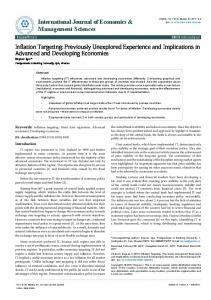
The following are observations on structural change in the Indian economy (involving agriculture and manufacturing) and would be well known. The data is extracted from the EPW Research Foundation database which reports time series data from sources like Central Statistics Office, Annual Survey of Industries, etc. We will also mention exact variables whenever required. The observations should be treated as broad indicators of structural change. The objective is to look at trends in the data. Supply side: The following chart (Figure 1) shows structural change from the supply side. The gross domestic product (GDP) is at factor cost (2004–05 series) at constant prices. Observations from Figure 1 form an empirical regularity across both developing (Verma 2012) and developed countries (for recent literature see World Economic and Social Survey 2006: Chapter 2, Memedovic 2009; Acemoglu 2009: Chapter 20). It is interesting to note that the manufacturing sector share has “crossed over” agricultural sector share very recently in India. 80
Figure 1: Evolution of Share of Agriculture and Manufacturing in GDP 0.5
A/Y
0.4 0.3 0.2
M/Y
0
1951 1954 1956 1959 1962 1964 1967 1970 1972 1975 1978 1980 1983 1986 1988 1991 1994 1996 1999 2002 2004 2007 2010 2012
0.1
Source: National Accounts Statistics of India, Sectoral GDP at Factor Cost (2004–05 series, at constant prices).
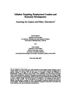
Let us also look at the sectoral growth rates over time in the last two decades and the simple averages of growth rates (Figure 2). The gap between the growth rates of manufacturing and agricultural sectors, on average, is 4.3% during 1994– 2013. The growth gap is approximately 2.9% post-independence and is 2.9% again during 1971–2013. Therefore, the growth gap has increased significantly in the last two decades. We will later use this fact to understand the relative price path over time using a simple macroeconomic model. Figure 2: Sectoral Growth Rate of Growth: Agriculture and Manufacturing 20
Manufacturing
15 Manufacturing average
10 5 0
2013
2011
2012
2010
2009
2007
2008
2005
2006
2003
2004
2001
2002
1999
2000
1997
1998
1996
1995
-10
Agriculture average
Agriculture
-5 1994
short- to medium-run, which in turn, would affect the structure of the economy over time. Inflation (as defined in subsection on “relative price change and inflation” later in this article) in developing economies then can be viewed as an intertemporal “equilibrating” variable that tries to achieve “balanced” growth across sectors in the long-run. Accordingly, inflation may be modelled either in terms of “equilibrium” dynamics (Bose 2011) or “disequilibrium” dynamics (Kalecki 1955; Cardoso 1981; Basu 2010) of the economy. The primary aim of this article is to link long-run movement in relative price to structural change in developing economies by using the method of “equilibrium dynamics” and to its implications for inflation targeting and the growth–inflation trade-off. Such an approach has not been explored in the recent literature that evaluates inflation targeting (Azad and Das 2013; Chandrasekhar 2014; Correa 2014; Kohli 2015; Mahajan, Saha and Singh 2014; Moorthy and Kolhar 2011; Nachane 2014; Patnaik 2014; Singh 2014), structural change (BinswangerMkhize 2013; Cortuk and Singh 2011, 2015; Reddy 2015; Verma 2012), and linkages between inflation and sectoral performances/dynamics (Guha and Tripathi 2014; Mishra and Roy 2011; Nair and Eapen 2015) in the Indian context. To motivate the discussion, the article first looks at structural change in India in the recent past: movement of output share, demand composition over time, relative price movement, and relative investment in agriculture and manufacturing sectors. We do not explore services sector here so as to focus on relative price movement between agriculture and manufacturing sectors. Next, the article builds a simple model to understand the link between relative price movements and associated structural change in a developing economy. Finally, the article comments on two contemporary issues: growth– inflation trade-off and inflation targeting in India by using the results of the models.
Source: National Accounts Statistics of India, Sectoral GDP at Factor Cost (2004–05 series, at constant prices).
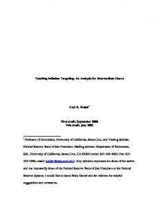
Demand side: Engel’s law in its simplest form says that a greater proportion of income is spent on non-agricultural goods and less is spent on necessities like food as household incomes rise. As a result, the ratio of expenditure on food to manufactured goods will decline over time. To get an estimate of expenditure shares, we have used private final consumption expenditure (PFCE) by object at constant prices (2004–05 series). For food consumption, the component “food” is taken from the head “food, beverages and tobacco” and for manufacturing consumption, we have added expenditures on “clothing and footwear” to that on “furniture, furnishing and appliances.” We expect income elasticity of “clothing and footwear” to be higher than that of “food” but lower than that of other manufactured goods. Since we are looking at two sectors, we have clubbed “clothing and footwear” with other manufactured goods. From Figure 3 (p 81), one can easily observe the manifestation of Engel’s law in India. In fact, food still occupies a considerable proportion of total expenditure (computed as manufacturing + food). Relative price movement: We define the relative price as the ratio of price of agricultural goods to that of manufactured january 14, 2017
vol liI no 2
EPW
Economic & Political Weekly
SPECIAL ARTICLE Figure 3: Expenditure Shares in India Structural Change: Demand Side 7
Food/Total
6 Food/Manufacture (right scale)
5
0.6
4 3
0.4
2
Manufacture/Total 0.2
0
Source: National Accounts Statistics of India, Domestic Savings, Capital Formation and Consumption.
Figure 4: Movement of Relative Price of Agriculture (1971–2014) 2 1.6 1.2 0.8
2013
2011
2009
2007
2003
2005
1999
2001
1997
1995
1991
1993
1987
1989
1985
1983
1979
1981
1975
1977
1971
1973
0.4
Source: Price Indices, WPI (base 2004–05).
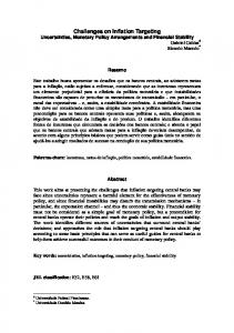
Figure 5: Movement of Relative Price of Agriculture (1994–2015) 2 1.6 1.2
p = 0.0041e 0.0001 t R² = 0.9422
0.8 0.4
April 2004 September 2004 February 2005 July 2005 December 2005 May 2006 October 2006 March 2007 August 2007 January 2008 June 2008 November 2008 April 2009 September 2009 February 2010 July 2010 December 2010 May 2011 October 2011 March 2012 August 2012 January 2013 June 2013 November 2013 April 2014 September 2014 February 2015
0
Source: Price Indices, WPI (base 2004–05).
Relative investment: One would expect that rising agricultural price at the margin would fetch more investment into the Economic & Political Weekly
EPW
january 14, 2017
vol liI no 2
1 0.8 0.6 0.4
2011
2013
2007
2009
2005
2001
2003
1997
1999
1995
1991
1993
1987
1989
1983
1985
1979
0
1981
0.2
1975
goods. This may also be called agricultural terms of trade. The data is obtained by dividing the Wholesale Price Index (base 2004–05) of food articles by that of manufactured products (Figure 4: 1971–2014, yearly data and Figure 5: 1994–2015, monthly data). Figure 4 shows that relative price started rising in the early 1980s. It is clear from Figure 5 that relative price has moved considerably in favour of agriculture in the time period 1994–2015. We have also added a trend line (Figure 5) to get a preliminary idea on the nature of change. The trend line seems to suggest an exponential path. Similar observations have been noted and the underlying factors have been discussed by Rajan (2014) and Krishnaswamy and Rajakumar (2015). One of the obvious factors is the rise in minimum support price (MSP). However, such a secular trend may also be an outcome of sectoral growth gap noted in an earlier subsection “supply side.”
0
1.2
1977
2011
2013
2007
2009
2005
2001
2003
1997
1999
1995
1991
1993
1987
1989
1983
1985
1979
1981
1975
1977
1971
0
1973
1
Figure 6: Relative Investment in Agricultural Sector Investment in Agriculture/Investment in Manufacture
1971
0.8
1973
1
sector. We compare gross fixed capital formation (GFCF) in agriculture to that in manufacturing (registered and unregistered) at constant prices (2004–05 series). Figure 6 shows that, relative investment in agriculture fell considerably in India. Therefore, it seems that relative price movement fails to explain relative investment.
Source: National Accounts Statistics of India, Domestic Savings, Capital Formation and Consumption.
Theories of Structural Change
The explanation of structural change requires description of alterations in the share of production, demand and employment from agriculture to manufacturing and then to services (Kuznets 1973). The models of structural change must be built around “non-balanced” growth at the sectoral level, but aggregate variables must follow a balanced growth path to be consistent with Kaldor’s facts such as long-run constancy of factor income share, interest rate and so on. The literature on structural change has tried to address nonbalanced growth from the demand and supply sides. The demand-side factors essentially incorporate Engel’s law through non-homothetic utility function (Kongsamut, Rebelo and Xie 2001), assuming that no imbalances feed in from the supply side. The supply-side explanation goes back to the work of Baumol (1967), who emphasised that “uneven growth” (nonbalanced growth) will be a general feature of growth process because different sectors will grow at different rates owing to different rates of technological progress. The price of goods in the sector growing at a higher rate would decline, inducing a substitution effect in favour of the same sector. A detailed discussion on the variation of these models can be found in Acemoglu (2009). Two recent studies in the Indian context are Verma (2012) and Binswanger-Mkhize (2013). However, structural change in developing economies like India probably comprises more than changes in sectoral share alone: production itself may be constrained by some “rigidity.” For instance, agricultural production may be affected by fragmented land, therefore, even if agricultural terms of trade were improving because of MSP (or for some other reason), investment in land will not increase production or productivity. In fact, because of rising MSP on foodgrain, farmers may not want to grow other commercial crops (Rajan 2014). However, a rising income (because of higher MSP and higher terms of trade) will (as per Engel’s law) cause a demand shift towards 81
SPECIAL ARTICLE
protein rich food (and towards other commercial crops) and a rise in their prices. This will lead to an overall increase in prices for necessities, a fall in real wages, and a further increase in MSP and/or nominal wages in the manufacturing sector. This may lead to what is known as wage–price spiral. If the manufacturing sector is able to pass the rising wage cost to the customer, then inflation in agricultural sector will percolate quickly to the entire economy. If the manufacturing sector is not able to pass the cost, then profit will be squeezed and investment in manufacturing sector will diminish hurting overall growth in the economy. Therefore, structural change in a developing economy like India must be understood keeping such distinguishing factors in mind. The production conditions of the agricultural sector and manufacturing sector may be quite different. It may not be possible to smoothly substitute capital for labour (or vice versa) in agriculture. This article picks up one particular issue amongst many that deserve attention: the issue of rising relative price of agricultural good in India and what that implies for inflation targeting. This is tested through a simple macroeconomic model, a model that is not specific to India but should be of general analytical interest. A Simple Macroeconomic Model
Supply and demand conditions: There are two sectors in the closed economy, industry (Y-sector) and agriculture (A-sector). There is surplus labour in A-sector, which produces food for self-consumption and for Y-sector. Let the food available for Ysector after netting out self-consumption be X, also known as “marketed surplus.” This surplus is fixed in the short-run. Let the relative price of food be p (=PA /PM). Marketed surplus, X, is consumed by Y-sector. The proceeds pX go to landowners and big traders of A-sector and is used to buy capital goods from Y-sector. This means that a rise in p (and hence in pX) does not cause this group to demand more food, thereby causing a fall in marketed surplus in the same period. If that happens, p would increase further, leading to explosive price path. Such possibility is ruled out by the assumption that demand for food by this group has already been satisfied and there are no further income and relative price effects on food demand. Let us assume that investment in A-sector increases productivity/output in such a manner that marketed surplus grows at a fixed rate X, the rate does not explicitly depend on relative price p. This may not be an unreasonable assumption as investment in agriculture does not seem to respond to relative price in India (Figure 6). Industry produces capital goods (I) and consumer durables (C). Output in the industrial sector is produced using constant returns to scale (CRS) technology: Y=F (K, L)=L ρ K 1 – ρ=K η ρ; where η = (L/K), the labour–capital ratio. Note also that Y = C + I, C and I are perfect substitutes and the relative price between C and I is unity. We assume that the product wage rate “w” (that is, the marginal product of labour) is fixed. In a general equilibrium framework, one expects wages to be driven down to zero with 82
surplus labour (the “complementary slackness” condition), but that is unlikely to be acceptable “socially” or “institutionally.” A fixed and positive wage (may beat a low level) is an accepted assumption in literature. Profit maximisation implies, MPL = w (product wage) 1
w 1
or, ρ η ρ – 1 = w, from which we get η =
As long as w is constant, (i) labour–capital ratio is constant, (ii) the rate of return to capital “r” is constant, and (iii) income share ratio wL/rK (in units of Y-goods) is constant. Now by property of CRS technology, Y/K=F(1, L/K)=F(1, η) = some constant, say B. Therefore, industrial output function can be written as Y=BK …(1) Since K is given historically in the short run, supply of industrial goods is fixed in the short run. Foregoing discussion also shows that income in Y-sector is given in the short run. Let a fraction “s” of industrial sector income Y be saved (S = sY) and reinvested back to Y-sector. So, growth rate of Y is given by:
g Y = Y K = I/K = sY/K = sB Y K
…(2)
Note: The dot over a variable’s notation implies time rate of change in the variable. Since, Y and K both grow at the same rate “sB,” by CRS technology, L also grows at the rate “sB.” This is the rate at which surplus labour is sucked out of A-sector. However, this rate is not constant, as “s” is not constant (see later subsection “Relation between p and industrial growth rate”). Let a fraction “α” of industrial sector income Y (production is equal to income in equilibrium) be spent on food (so fraction (1 – α – s) is spent on consumer durables). Demand for food from industrial sector is given by αY. Market clearing in the short run: In the short run, demand– supply balance for food is given by: αY = pX or (α/p) = X/Y …(3) The left-hand side is the relative demand for food and the right-hand side is relative supply of food. The relative demand is a downward sloping schedule in p, with the usual assumptions that demand for food is price and income inelastic. Note that, at any given period, the relative supply of food (X/Y) is fi xed, because both X and Y are fi xed in the short run. So p must change to clear the market in the short run. This balance determines short-run relative price (Figure 7, p 83). Relation between p and industrial growth rate: Consider the effect of a rise in p on industrial growth rate. What happens to the total expenditure on food (X) and consumer durables (C) when p rises? Rise in p (say caused by a rise in price of food) causes demand for X to contract. Demand for X is price inelastic, so expenditure on X increases. A fall in demand for X causes rise in demand for C (that is, cross-price elasticity is not zero, which is possible only with “non-homothetic” utility function). At the same price of C, expenditure on C increases, leading to an increase in total expenditure on X and C, given january 14, 2017
vol liI no 2
EPW
Economic & Political Weekly
SPECIAL ARTICLE Figure 7: Short-run Price Determination p
p0
Į(p) α/p
X/Y
Relative demand and supply of food
by (C + pX). With a given level of income in Y-sector, saving reduces. So s = s(p) with s′(p) < 0. Therefore, gY is a decreasing function of p. A rise in p slows down the growth rate of Y-sector. This relation can be written as: gY = s(p)B; s′(p) < 0 …(4) Relative price change and inflation: Note that this model does not have money explicitly, the focus is on the real side of the economy. Usually, inflation is defined as a rise in prices in terms of money; therefore we must now define what inflation in our model is. The equilibrium price in the short run is established (starting from “any” price) through movement along relative demand and supply curves. This is the usual Marshallian price adjustment to maintain demand–supply balance in the short-run. Assuming that the adjustment is stable, the market will clear in the same period (adjustment is instantaneous). Such one shot or instantaneous adjustments in relative price is not treated as inflation in this article. The other type of price adjustment involves changes in the equilibrium relative price. The market clearing relative price may increase or decrease over time because of shifts in the relative demand and supply curves over time due to changes in the parameters that are exogenous in the short run. Such a sustained rise in equilibrium relative price is treated as inflation in this article. There are examples of macro-models that are concerned with inflation without explicitly introducing money or separate money market equilibrium. For instance, in Kalecki (1955), inflation can be viewed as falling real wages of workers. In our model, the product wage rate in Y-sector is fixed, and hence, a rise in p causes real wages in terms of food to decrease. Another example is Cardoso (1981), in which there is no explicit money or money market. There, inflation is a continuous change in relative price arising out of structural disequilibrium captured through “disequilibrium dynamics” (also see Basu 2012: ch 4). Long-run p and structural change: Figure 7 shows the static balance in the economy at a point in time. What happens to Economic & Political Weekly
EPW
january 14, 2017
vol liI no 2
the economy over time? Is the short-run p the long-run p as well? It depends on what happens to relative demand and supply curves over time. The relative demand curve already captures any changes in p (movement along the curve). The relative supply curve would shift depending on relative growth rates of X and Y. If agricultural output is growing (g X) faster than industrial output (g Y ), then (X/Y) would rise and vice versa. A rise in (X/Y) causes short-run p to fall, whereas a fall in (X/Y) causes short-run p to rise. Which case is more likely? Figure 2 shows that the manufacturing sector (industrial sector in the model) on the average is growing at a faster rate in India. Therefore initially we have gY > g X. This growth gap causes relative supply of food (X/Y) to fall over time and p to rise over time. A rise in p causes industrial growth to slow down (equation 4) with g X = X . This leads to closing of the initial growth gap over time. Once the gap is completely closed, p reaches its long run value, say p . This sustained rise in short-run market clearing p (from p0 to p ) is treated as inflation here. At p , g Y = g X = X, that is, all the sectors grow at the exogenously given growth rate of marketed surplus of food. This is nothing but the “balanced” growth result. Since overall growth rate of the economy is the weighted average of sectoral growth rates, in the long run, economy’s growth rate converges to the “slow” growing sector. This result also highlights the fact that, even if the economy starts with a high growth rate in industrial sector, long run growth rate cannot remain above agricultural growth rate. More the growth gap (= gY – gX) to begin with, faster is the rise in p and quicker is the fall in relative supply (X/Y) initially. As the growth gap closes, the rate of rise in p decreases and p asymptotically reaches to its long-run value p . Consequently, (X/Y) also reaches a stable value. The fall in (X/Y), that is, falling share of agriculture is nothing but “structural” change. The overall growth rate of the economy being a weighted average of industrial and agricultural growth rates, overall growth rate is higher than agricultural growth rate initially and gradually decreases with a rise in p, finally approaching asymptotically to agricultural rate of growth. Therefore, starting with an initial growth gap, economy achieves balanced growth through continuous adjustment in market clearing price over time which in turn gives rise to structural change. Relative price movement and structural change are endogenously determined in the model. Figures 8, 9 and 10 (p 84) capture these results. One can now easily compare the actual relative price path noted in Figures 4 and 5 to that of price path (initial stages) in Figure 10. Discussion
Growth–inflation trade-off? Overall growth rate in the economy is a weighted average growth rate of industrial and agricultural sector growth rates. Now, the rate of rise in p (inflation) is an increasing function of growth gap. A one-shot rise in agriculture sector growth rate (at any date) increases overall growth rate, reduces the growth gap and reduces 83
SPECIAL ARTICLE Figure 8: Long-run Price Determination and Structural Change
Figure 10: Behaviour of Relative Price and Output Composition (Y/X) Over Time
p
X
p, Y/X
p, (Y/X)*
2 leading to rise in shortrun p
1 Growth gap causes (X/Y) to fall
p p0
t (X/Y)*
X/Y
Relative demand and supply of food
Figure 11: Effect of a Rise in Sectoral Growth Rates on Price Path p
Figure 9: Adjustment of p to Its Long-run Value and Structural Change p
Agri-sector
p high higher gYY higher
α/p Į(p)
p
p p0 Initial growth Initial growthgap gap X/Y
(X/Y)*
X
Industrial sector Growth rates
relative price inflation at any subsequent date. In Figure 9, the agricultural sector growth curve shifts right, reducing the growth gap at any given p. The long-run p would be lower now, with the new price path having a gentler slope (Figure 11). In this case, there is no “trade-off” between growth and inflation. Note also that, since the economy achieves balanced growth by approaching the slow-growing sector, a rise in the growth rate of the slow-growing sector (here agricultural sector) would permanently raise overall growth rate at all dates. On the other hand, an attempt to raise industrial growth rate increases the overall growth rate, but increases the growth gap as well. This causes long-run p to increase with the new price path having a steeper slope resulting in increased inflation (Figure 11). Further, the rise in the overall growth rate is only temporary. There exists the growth–inflation trade-off when an attempt is made to increase overall growth of the economy by pushing up the growth rate of the faster growing sector. Therefore, overall growth can be increased without any adverse consequence on inflation if the growth bottleneck of the slow-growing sector is alleviated. Inflation targeting: Reserve Bank of India (RBI) adopted the Consumer Price Index (combined) as the nominal anchor for conducting monetary policy in February 2015. The basis for this was laid out in the RBI report (2014) titled “Revise and Strengthen the Monetary Policy Framework” (popularly known as the Urjit Patel Committee Report). The recommended target is 4% inflation with a band of +/– 2% which is to be achieved in the next two years through a “glide path” (RBI 2014: 20). The glide path essentially shows the downward movement of intermediate inflation targets over time. We use the properties of the model to make a few comments on such glide path for a developing economy. 84
higher ggXX higher
p low
t Figure 12: The Glide Path and Effect of Higher Sectoral Growth Rates on Inflation
ʌ ʌ0
gY gX
t It may be noted that the objective here is not to evaluate whether inflation targeting as a policy is appropriate for India, but to understand how glide path may be derived from the dynamics of the real side of the economy and to perform simple comparative static exercises graphically. We emphasise that there is a “real” side to the glide path, apart from the monetary side story. Inflation targeting may be viewed here as targeting a particular level of relative price at a given date. There is however one important difference; glide path is “chosen” by the RBI, whereas in our case, it is an endogenous property of the model. From the price path (Figure 10), a glide path is derived from the slope of .the price path at each point in time (noting that p inflation is p ). A rise in agricultural growth rate (the slowgrowing sector) generates a favourable glide path, while a rise in industrial growth rate generates an unfavourable glide path. This can be derived from Figure 11 (also see Figure 12, inflation is denoted by ). Our model shows that, any policy that aims to increase the growth rate of the industrial sector widens the growth gap bet ween industrial and agricultural sectors, accelerates inflation and pushes up the intermediate target of inflation. january 14, 2017
vol liI no 2
EPW
Economic & Political Weekly
SPECIAL ARTICLE
The lesson is clear: unless something is done to increase agricultural growth rate, an attempt to raise industrial growth rate alone will render the job of inflation targeting difficult. Conclusions
This article has tried to establish that relative price inflation, growth and structural change in developing economies are intrinsically connected. In developing economies, some sectors may have rigid production structures or prices may adjust faster in some sectors than in other sectors. Further, unlike the standard models of structural change, it cannot be assumed that all the sectors will have standard neoclassical production functions with smooth factor substitution. Developing economies have underdeveloped financial markets and resale markets for capital goods. Labour laws do not permit a substitution with capital for an existing productive activity. Agricultural production also does not keep pace with changing consumption baskets, partly because of controlled prices for foodgrains. The results of our simple model show that the price path is related to the dynamics arising out of initial imbalances in sectoral growth rates. The short-run market clearing price achieves the usual demand–supply balance at a point in time. The changes in market clearing price over time is an outcome
References Acemoglu, Daron (2009): Introduction to Modern Economic Growth, New Jersey: Princeton University Press. Azad, Rohit and Anupam Das (2013): “Inflation Targeting in Developing Countries: Barking Up the Wrong Tree,” Economic & Political Weekly, Vol 48, No 41, pp 39–45. Basu, Kaushik (2012): Analytical Development Economics: The Less Developed Economy Revisited, New Delhi: Oxford University Press. Baumol, William J (1967): “Macroeconomics of Unbalanced Growth: The Anatomy of Urban Crisis,” American Economic Review, Vol 57, pp 415–26. Binswanger-Mkhize, Hans P (2013): “The Stunted Structural Transformation of the Indian Economy,” Economic & Political Weekly, Vol 48, Nos 26 and 17, pp 5–13. Bose, Amitava (2011): “Inflation and Growth: Long Run Pulls,” Unpublished Manuscript, IIM Calcutta. Cardoso, Eliana (1981): “Food Supply and Inflation,” Journal of Development Economics, Vol 8, No 3, pp 269–84. Chandrasekhar, C P (2014): “Off-target on Monetary Policy,” Economic & Political Weekly, Vol 49, No 9, pp 27–30. Correa, Romar (2014): “And a Little Child Shall Lead You: Through the Thicket of the Urjit Patel Report,” Economic & Political Weekly, Vol 49, No 9, pp 30–32. Cortuk, Orcan and Nirvikar Singh (2011): “Structural Change and Growth in India,” Economics Letters, Vol 110, pp 178–81. — (2015): “Analysing the Structural Change and Growth Relationship in India State-level Evidence,” Economic & Political Weekly, Vol 50, No 24, pp 91–98, Guha, Atulan and Ashutosh Kr Tripathi (2014): “Link between Food Price Inflation and Rural Wage Dynamics,” Economic & Political Weekly, Vol 49, Nos 26 and 17, pp 66–73. Economic & Political Weekly
EPW
january 14, 2017
of the maintenance of dynamic balance (by shift in relative supply curve) over the long run. The convergence of sectoral growth rates drives the structural change. Achieving dynamic balance depends on how sectoral supply curves respond to relative price change. In our model, the industrial sector’s growth responds negatively to an increase in relative price. In developing economies, the agricultural sector has a large share to begin with, and the model shows how such an initial imbalance leads to eventual rise in relative price of agriculture and accompanying structural change. Since price change is required to achieve dynamic balance over long run, study of inflation must go beyond the usual short-run analysis of output–inflation trade-off. One can of course study short-run properties of the price path due to change in exogenous parameters, like changes in MSP, etc. However, a one shot change in exogenous parameter cannot stop increase in the relative price as long as sectoral growth imbalances persist. Short-run policy must, therefore, be consistent with growth path of the real sectors, driven by underlying economic structure. Our finding is that the dynamics of the real sector play a paramount role in changes in relative price and thus in structural change. Policies that attempt to rectify sectoral imbalances are as important as monetary policies that tackle inflation in developing economies.
Kalecki, Michael (1955): “The Problem of Financing of Economic Development,” Indian Economic Review, Vol 2, No 3, pp 1–22. Kohli, Renu (2015): “Inflation Targeting as Policy Option for India Evaluating the Risks,” Economic & Political Weekly, Vol 50, No 2, pp 10–14. Kongsamut, Piyabha, Sergio Rebelo, and Danyang Xie (2001): “Beyond Balanced Growth,” Review of Economic Studies, Vol 48, pp 869–82. Krishnaswamy, R and Dennis J Rajakumar (2015): “Recent Trends in Inter-Sectoral Terms of Trade,” Economic & Political Weekly, 50, No 5, pp 82–84. Kuznets, S (1973): “Modern Economic Growth: Findings and Reflections,” American Economic Review, 63, 247–58. Mahajan, Saakshi, Souvik Kumar Saha and Charan Singh (2014): “Inflation Targeting in India,” Indian Institute of Management Bangalore Working Paper: 449. Memedovic, Olga (2009): “Structural Change in the World Economy: Main Features and Trends,” United Nations Industrial Development Organization, Working Paper No 24. Mishra, Prachi and Devesh Roy (2011): “Explaining Inflation in India: The Role of Food Prices,” http://www.prachimishra.net/mishra_roy_reviseddraft_ipf_oct25’. Moorthy, Vivek and Shrikant Kolhar (2011): “Rising Food Prices and India’s Monetary Policy,” Indian Institute of Management Bangalore Working Paper: 325.
Nachane, D M (2014): “Flawed Cartography? A New Road Map for Monetary Policy,” Economic & Political Weekly, Vol 49, No 9, pp 24–26. Nair, Sthanu R and Leena Mary Eapen (2015): “Agrarian Performance and Food Price Inflation in India: Pre- and Post-economic Liberalisation,” Economic & Political Weekly, Vol 50, No 31, pp 49–60. Patnaik, Prabhat (2014): “On Controlling Inflation,” Economic & Political Weekly, Vol 49, No 45, pp 44–48. Rajan, Raghuram (2014): “Fighting Inflation,” RBI Monthly Bulletin, March, pp 11−20. Reddy, Amarender (2015): “Growth, Structural Change and Wage Rates in Rural India,” Economic & Political Weekly, Vol 50, No 2, pp 56–65. RBI (2014): “Report of the Expert Committee to Revise and Strengthen the Monetary Policy Framework,” Reserve Bank of India, Mumbai. Singh, Charan (2014): “Inflation Targeting in India: Select Issues,” Indian Institute of Management Bangalore Working Paper: 475. Verma, Rubina (2012): “Structural Transformation and Jobless Growth in the Indian Economy,” The Oxford Handbook of the Indian Economy, Chetan Ghate (ed), New York: Oxford University Press. World Economic and Social Survey (2006): “Diverging Growth and Development,” United Nations.
EPW Index An author-title index for EPW has been prepared for the years from 1968 to 2012. The PDFs of the Index have been uploaded, year-wise, on the EPW website. Visitors can download the Index for all the years from the site. (The Index for a few years is yet to be prepared and will be uploaded when ready.) EPW would like to acknowledge the help of the staff of the library of the Indira Gandhi Institute of Development Research, Mumbai, in preparing the index under a project supported by the RD Tata Trust. vol liI no 2
85