Modelling and Simulation in Materials Science and Engineering, Vol. 17, no. 4, 045004 (2009)
Influence of representative volume element size on predicted elastic properties of polymer materials P K Valavala1, G M Odegard1 and E C Aifantis2 1
Department of Mechanical Engineering-Engineering Mechanics, Michigan Technological University, Houghton, MI 2 College of Engineering, Michigan Technological University, Houghton, MI E-mail:
[email protected] Abstract. Molecular dynamics (MD) simulations and micromechanical modeling are used to predict the bulk-level Young’s modulus of polycarbonate and polyimide polymer systems as a function of representative volume element (RVE) size and force field type. The bulk-level moduli are determined using the predicted moduli of individual finite-sized RVEs (microstates) using a simple averaging scheme and an energy-biased micromechanics approach. The predictions are compared to experimental results. The results indicate that larger RVE sizes result in predicted bulk-level properties that are in closer to the experiment than the smaller RVE sizes. Also, the energy-biased micromechanics approach predicts values of bulk-level moduli that are in better agreement with experiment than those predicted with simple microstate averages. Finally, the results indicate that negatively-valued microstate Young’s moduli are expected due to nanometer-scale material instabilities, as observed previously in the literature.
1. Introduction Nanostructured materials have received significant attention in recent years due to their potential to provide gains in specific stiffness and specific strength relative to traditional materials for engineering applications. The efficient development of these materials requires simple and accurate structure-property relationships that are capable of predicting the bulk mechanical properties of as a function of the molecular structure and interactions. Modeling techniques spanning over multiple length scales must be used to establish these structure-property relationships. At the atomistic length scale, molecular dynamics (MD) has been shown to be a powerful technique for predicting the equilibrated molecular structures of polymer-based materials for a given thermodynamic state [1-6]. The mechanical behavior of such material systems can be studied with the aid of a representative volume element (RVE) that is capable of quantitatively depicting the macro-scale characteristics. RVEs have been extensively used in the constitutive modeling of both crystalline and amorphous materials [7-11]. However, central to this methodology is the choice of the RVE that can accurately capture the material’s bulk-scale mechanical behavior. The optimal choice of an RVE for an amorphous nanostructured material remains a challenge. Although traditional methodologies have been applied to continuous materials [8], selection of nanometer-sized RVEs for discrete polymer structures has not been rigorously addressed [12]. Ostoja-Starzewski has proposed establishing a statistical volume element (SVE) that approaches an RVE under certain limiting conditions [9, 10]. A multiscale modeling approach has been recently developed to account for a range of conformational microstates of a polymeric network must be accounted for [13], where a microstate refers to a single equilibrated nanometer-sized RVE with a unique molecular structure (polymer network). In these studies, physically-motivated statistical weighting of properties obtained from individual microstates for each polymer were utilized to establish
1
Modelling and Simulation in Materials Science and Engineering, Vol. 17, no. 4, 045004 (2009) bounds of the predicted moduli and are subsequently compared to experimentally-measured values of moduli for these materials. The mechanical response of polymers is a consequence of the short- and long-range interactions of the constituent molecular chain network. The finite-chain network can only sample a small portion of the conformational space of the bulk polymer. As a result, the physical properties of a polymer can vary substantially on the nanometer length-scale [14-23]. Similarly, the RVE size can influence the predicted mechanical properties of a polymer [24] using multiscale modeling techniques. Increasing the RVE size of a modeled polymer establishes predicted physical properties over a larger conformational space. The effect of the molecular RVE size on predicted polymer properties in multiscale models of polymers needs to be rigorously investigated. In this study, a multiscale modeling technique has been used to predict the bulk elastic moduli of polyimide and polycarbonate material systems using different RVE sizes and two different force fields. Multiple microstates for each RVE size were considered. The calculated weighted average for the microstates of each RVE size was found to be in good agreement with the experimentally measured properties. Also, it was found that increasing the RVE size provided evidence for a convergence to limiting values, as expected from data from bulk-scale experiments. The results of this study demonstrate this conclusion for the first time using a statistical-based multiscale modeling method [13]. 2. Molecular Modeling Figure 1 shows the polymer repeat units for the two polymer materials used in the current study. MD simulations were carried out on two polymer materials, a polyimide and a polycarbonate. Three different RVE sizes were modeled for the two polymer materials. Nine independently-established thermallyequilibrated structures were obtained for each polycarbonate RVE size. For polycarbonate, the smallest RVE consisted of 3,972 atoms with 6 polymer chains; the medium-sized RVE had 5,958 atoms with 9 polymer chains and the largest RVE had 7,944 atoms with 12 polymer chains. All polycarbonate chains for the different RVE sizes had 20 repeat units per chain. Each of the nine structures for each RVE size represents a microstate for the polycarbonate system. For the polyimide system, the smallest RVE consisted of 4,244 atoms with 7 polymer chains; the medium sized RVE consisted of 6,622 atoms with 11 polymer chains, and the largest RVE consisted of 8,248 atoms with 14 polymer chains. Each polyimide chain consisted of 10 repeat units per chain. A total of nine RVEs were established for the small and the large models of polyimide and seven for the medium-sized RVE. Similar to polycarbonate, each polyimide model represented a single microstate for the corresponding RVE size. The chain lengths were chosen to be the same as used previously [13]. The above-described procedure was identically used for both the AMBER and OPSL-AA force fields, as implemented in the TINKER modeling package. The functional forms of these force fields are described in greater detail elsewhere [6]. The published values of Tg for the polycarbonate and polyimide systems are 145 and 211°C, respectively [25, 26]. All RVE structures were initially prepared in a gas-like phase with extremely low densities. For each RVE sample, the polymer chains were placed in a simulation box with random conformations and orientations. Energy minimization simulations were conducted initially without periodic boundary condition to relax individual chains. Afterwards, the periodic boundary conditions were applied and a series of minimizations were carried out at gradually-increasing densities. The MINIMIZE and NEWTON subroutines of the TINKER modeling package were used for these minimizations, which correspond to a quasi-Newton L-BFGS method [27] and a truncated Newton energy minimization method [28], respectively. The minimizations were performed to RMS gradients of 1×10⁻² and 1×10⁻⁵ kcal/mole/Å, respectively.
2
Modelling and Simulation in Materials Science and Engineering, Vol. 17, no. 4, 045004 (2009) Once each of the RVEs were established with the approximate solid bulk density, a series of MD simulations were used to establish thermally-equilibrated solid structures in the following order at 300 K: (1) a 50 ps simulation with the NVT (constant number of atoms, volume, and temperature) ensemble to prepare the structure for further equilibration, (2) a 100 ps simulation with the NPT (constant number of atoms, pressure, and temperature) ensemble at 100 atm to evolve the system to higher densities as the structure was prepared from a low density structure, (3) a 100 ps NPT simulation at 1atm to reduce the effects of high-pressure simulations and to let the system evolve to a state of minimal residual stresses, and (4) a 100 ps NVT simulation to allow the system to equilibrate at the simulated temperature and density for a specific microstate. The DYNAMIC subroutine of the TINKER modeling package was used for the MD simulations with periodic boundary conditions. Examples of the molecular models that were established in a manner described above are shown in Figure 1. The final specific weight of each RVE was approximately between 1.1 and 1.2. A total of 115 RVEs were modeled for the current study. These simulations were all conducted at 300 K for two reasons. First, stable amorphous structures of the polymers could be established at this temperature. Second, because it is expected that the glass transition temperature of these two systems is much higher than 300 K, the calculated elastic properties should not be significantly influenced by the thermal history of the system. It is important to note that although engineering polymers are subjected to loads on time scales that are orders of magnitude above 1 second in engineering practice, limited computational resources restricted simulation times for establishing molecular structures on the order of hundreds of picoseconds.
Polyimide Polyimide
Polycarbonate Polycarbonate
Figure 1. Schematics of the polymeric chain repeat units and the corresponding representative volume elements for polyimide and polycarbonate.
3. Equivalent-Continuum Properties An equivalent-continuum modeling approach was used to determine the equivalent-continuum mechanical properties of each RVE (microstate). A hyperelastic-continuum constitutive relation [6] was used to model the elastic behavior of the equivalent-continuum material models. The constitutive relationships of these models had the following characteristics: (1) isotropic material symmetry due to the amorphous molecular structures, (2) finite-deformation framework, (3) expressed in terms of volumetric (shape preserving) and isochoric (shape changing) contributions, and (4) established using a thermodynamic potential. The assumed form of the equivalent-continuum strain energy is Ψ c = ψ vol + ψ iso
where
3
(1)
Modelling and Simulation in Materials Science and Engineering, Vol. 17, no. 4, 045004 (2009)
ψ vol = c1Ω1 ψ iso = c2 Ω 2
(2)
and Ω1 = ( I 3 − 1)
2
⎛ I ⎞ I3 Ω2 = ⎜ 11 3 + 22 − 30 ⎟ I I 3 ⎝ 3 ⎠
(3)
The parameters Ω1 and Ω2 in Equation (3) represent the volumetric and isochoric components of the strain-energy density; c1 and c2 are constants which represent material properties; and I1, I2, and I3 are the scalar invariants of the right Cauchy-Green deformation tensor, C. The second Piola-Kirchhoff stress tensor is therefore [6] S=
⎛ I1 ⎛ 1 I 23 ⎞ ⎤ −1 I1 I 2 2 ⎞ I 22 2⎡ ⎢6c1 I 3 ( I 3 − 1) − c2 ⎜ 1 3 + 6 2 ⎟ ⎥ C + 2c2 ⎜ 1 3 + 3 2 ⎟ I − 6c2 2 C 3 ⎢⎣ I 3 ⎠ ⎥⎦ I3 ⎠ I3 ⎝ I3 ⎝ I3
(4)
where I is the identity tensor. Equation (4) contains material parameters c1 and c2 which were evaluated for each microstate by equating the equivalent-continuum strain energy and the molecular potential energy for a set of identical deformation fields applied to the equivalent continuum and the molecular models [29]. For the molecular models, the strain-energy densities are computed from the force field using
Ψm =
1 Λ m − Λ 0m ) ( V0
(5)
where, Λ 0m and Λ m are the molecular potential energies before and after application of the deformations, which are directly computed from the force field, and V0 is the volume of the simulation box in the undeformed state. Two sets of finite deformations were applied to each of the RVEs and the equivalent-continuum in incremental steps. The molecular potential energy was calculated for each deformation using molecular statics. Specifically, for each deformation, an energy minimization was performed with periodic boundary conditions. The MINIMIZE and NEWTON subroutines of the TINKER modeling package were used for the energy minimization in the same manner as described above. For the volumetric deformation, volumetric strains (E11= E22 = E33 where E is the Green strain tensor) of 0.1%, 0.2%, 0.3%, 0.4% and 0.5% were applied. For the isochoric deformations, three-dimensional shear strain levels of γ23 = γ13 = γ12 = 0.1%, 0.2%, 0.3%, 0.4% and 0.5% (γij = 2Eij when i ≠ j) were applied. By equating the energies of deformation for the RVEs and the equivalent continuum for each of the two deformation types, the elastic properties were determined as described in detail elsewhere [6]. 4. Effective Polymer Properties The equivalent-continuum properties of each RVE obtained as described in the previous section was used to determine effective bulk properties of the polymer materials for each of the RVE sizes. The equivalentcontinuum properties represent the deformation response of the particular chain arrangements associated with the RVEs. It is expected that the approach described in the previous section will generally yield
4
Modelling and Simulation in Materials Science and Engineering, Vol. 17, no. 4, 045004 (2009) different predicted properties for different RVEs (for a given RVE size). Each of the RVEs is of the order of a few nanometers in length. However, the bulk-polymer response is an average mechanical response of the large number of RVEs that are statistically probable for a given polymer system. Due to the computational time and cost associated with establishing every possible conformational microstate for a polymer system, the modeling procedure described herein approximates the bulk material behavior with only a finite number of RVEs obtained as described in Section 2. To this end, the bulk polymer elastic behavior of each polymer system was determined using a physically-motivated weighted-averaging scheme. The details of this scheme have been described in detail elsewhere [13], but are briefly discussed below in the context of the current study for completeness. The Voigt model (rule-of-mixtures) assumes that the strains in all of the phases of a composite material are the same for a given bulk-level deformation. As a result, the predicted properties of a composite from the Voigt model corresponds to the upper bound of possible bulk elastic properties [30]. This approach provides a simple estimate of the expected properties for a material composed of phases or microstates of varying properties. The Voigt model prediction for a material with arbitrary number of constituents is given by, N
LV = ∑ cr L r
(6)
r =0
where LV are the effective stiffness tensor associated with the Voigt estimate; L r is the stiffness tensor components of phase r ; N is the total number of microstates considered; and cr is the volume fraction of phase r where N
∑c r =0
r
=1
(7)
Although better estimates for multi-phase materials have been established for composite materials [31], these generally assume a more specific geometry of the phases, such as fibrous or spherical reinforcements. Because the exact geometric shapes of the microstates considered herein are unknown, Equation (6) was utilized to estimate the bulk mechanical properties of the two polymer systems. The evaluation of the properties based on the Voigt approach is dependent on the volume fractions of the constituent microstates, as indicated by Equation (6). However, the distribution of microstates in a polymer material is generally unknown. A simple approach for selecting the relative volume fractions of the phases was recently proposed [13]. For this approach, it is assumed that the volume fraction of a particular microstate is equal to the probability of its existence so that cr in Equation (6) is replaced by the probability pr . Because there are no well-established distribution functions that describe pr for an amorphous polymer material, assumed forms of the function have been proposed [13]. For the research described herein, it was assumed that pr is determined using a physically-intuitive distribution that is biased based on the equilibrium potential energy of a particular microstate. Many engineering polymers operate much below the glass transition temperature, and thus exist in a glassy state. Due to the statistical nature of the growth of polymer networks during polymerization of addition polymers [32], the networks do not crystallize due to steric hindrance. It is expected that the lower-energy microstates are thermodynamically favored, with a higher probability than high-energy microstates. This approach has been shown to provide accurate estimates for the mechanical properties of polymers [13]. Motivated by this argument, a probability distribution function that satisfies this requirement is
5
Modelling and Simulation in Materials Science and Engineering, Vol. 17, no. 4, 045004 (2009)
pr =
Λ r −1 N
∑ (Λs )
−1
(8)
s =1
where N is the total number of different microstates considered and Λ r is the potential energy of microstate r calculated using the functional forms of each force field [6]. The definition in Equation (8) satisfies the requirement analogous to (7) N
∑p r =1
r
=1
(9)
More detail on this modeling approach can be found elsewhere [13]. Although the resulting distribution predicted by Equation (8) is similar to that predicted by the Boltzmann distribution, Equation (8) has been chosen to more accurately represent the modeled systems. The Boltzmann distribution describes the probability of occurrence of different states for a single given temperature. However, the peculiar nature of the energy landscape of polymer glasses is the presence of high energy barriers that may restrict transitions from higher energy basins to lower energy basins. These high energy barriers are due to the presence of significant steric hindrances in the network. Computationally, the high energy barriers can be further exaggerated due to the limited time steps that can be efficiently performed with MD techniques. In effect, this leads to a modeled material with configurations that would thermodynamically correspond to higher temperatures than that of the ambient reservoir. As a result, the actual distribution of microstates in a glassy polymer can be modeled as having a more even distribution along different energy levels than that described by the Boltzmann distribution. Therefore, the more distributed distribution described by Equation (8) is more appropriate for the polymer systems modeled herein. 5. Results and Discussion Tables 1-12 summarize the results obtained for each microstate for the two different polymers for OPLSAA and AMBER force fields. For each microstate, the methodology outlined in Section 3 was utilized for homogenization to predict the equivalent-continuum properties. It was found that there was a significant variation in the predicted properties for the various microstates. The deformation response for a polymer system is a consequence of the elaborate molecular chain network. As these microstates sample different conformational space in the molecular models, it is expected that they exhibit a wide range of properties. A previous study also indicated a large variation in the local mechanical properties of amorphous polymers [12]. It was also reported that there was a strong correlation between the size of the simulated model and the variation in the predicted properties with a wider distribution in properties observed at smaller RVE sizes. It is important to note that the method that was used to build the molecular models may have an influence on this observed behavior. As explained above, the preparation of the samples was via a random placement of chains in the simulation box. Because of the bulky aromatic rings in the polymer chains, there is an increased likelihood of significant steric hindrances preventing the microstates from achieving lower energy states. While other approaches to establishing molecular structures have been used, such as hybrid Monte Carlo-MD techniques and the simulated growth of polymer chains from the monomeric melt, it is still unclear how the method of preparation might lead to more consistent network models and thus predicted mechanical properties.
6
Modelling and Simulation in Materials Science and Engineering, Vol. 17, no. 4, 045004 (2009) Table 1. Microstate properties for the small RVE size of polycarbonate with AMBER Young’s Shear Density Λr Microstate modulus modulus (kcal/mole) (g/cc) (GPa) (GPa) 482.91 1.14 26.60 9.75 1 3872.13 1.14 6.22 2.15 2 23001.84 1.14 20.10 7.25 3 25470.26 1.13 11.50 3.99 4 27832.29 1.14 4.90 1.68 5 30000.92 1.10 4.87 1.66 6 31939.19 1.11 1.29 0.43 7 33221.32 1.14 6.57 2.24 8 36176.15 1.13 -1.92 -0.64 9 23555.67 1.13 8.90 3.17 Average 12780.03 0.02 9.12 3.34 Std. Dev. Table 2. Microstate properties for the medium-sized RVE of polycarbonate with AMBER Young’s Shear Density Λr Microstate modulus modulus (kcal/mole) (g/cc) (GPa) (GPa) 13,706.69 1.09 2.29 0.78 1 13,722.27 1.12 5.14 1.77 2 15,905.73 1.07 2.01 0.68 3 18,093.05 1.11 12.00 4.21 4 21,674.48 1.15 20.90 7.65 5 23,372.80 1.11 0.09 0.03 6 38,850.61 1.12 5.69 1.95 7 50,629.76 1.09 7.08 2.44 8 55,728.69 1.03 1.65 0.56 9 27964.89 1.10 6.32 2.23 Average 16250.79 0.03 6.55 2.39 Std. Dev. Table 3. Microstate properties for the large RVE size of polycarbonate with AMBER Young’s Shear Density Λr Microstate modulus modulus (kcal/mole) (g/cc) (GPa) (GPa) 16523.09 1.02 0.97 0.32 1 32070.92 1.04 6.54 2.28 2 35512.99 1.05 2.31 0.78 3 36568.99 1.08 6.54 2.24 4 37445.09 1.11 9.33 3.25 5 37548.48 1.04 14.3 5.34 6 45790.31 1.10 3.44 1.17 7 56070.49 1.11 8.06 2.80 8 68552.23 1.12 1.90 0.64 9 40675.84 1.07 5.92 2.09 Average 14838.23 0.04 4.28 1.59 Std. Dev.
7
Modelling and Simulation in Materials Science and Engineering, Vol. 17, no. 4, 045004 (2009) Table 4. Microstate properties for the small RVE size of polycarbonate with OPLS-AA Young’s Shear Density Λr Microstate modulus modulus (kcal/mole) (g/cc) (GPa) (GPa) 297.58 1.17 3.27 1.10 1 2123.78 1.16 1.55 0.53 2 21236.35 1.15 -0.12 -0.04 3 27204.39 1.15 11.50 3.98 4 30984.07 1.15 3.01 1.01 5 33364.17 1.15 1.08 0.36 6 33826.32 1.12 7.32 2.52 7 35127.00 1.14 4.20 1.42 8 39157.65 1.16 1.40 0.47 9 24823.48 1.15 3.69 1.26 Average 14310.28 0.01 3.64 1.26 Std. Dev. Table 5. Microstate properties for medium-sized RVE of polycarbonate with OPLS-AA Young’s Shear Density Λr Microstate modulus modulus (kcal/mole) (g/cc) (GPa) (GPa) 12398.52 1.15 3.80 1.28 1 12492.38 1.09 5.16 1.76 2 17059.73 1.11 3.81 1.30 3 19048.08 1.09 8.11 2.82 4 24761.87 1.12 3.91 1.28 5 25743.50 1.15 7.67 2.63 6 44663.33 1.13 0.06 0.02 7 56942.82 1.09 3.11 1.06 8 59766.92 1.04 0.62 0.20 9 30319.68 1.11 4.03 1.38 Average 18625.79 0.03 2.73 0.94 Std. Dev. Table 6. Microstate properties for the large RVE size of polycarbonate with OPLS-AA Young’s Shear Density Λr Microstate modulus modulus (kcal/mole) (g/cc) (GPa) (GPa) 13530.63 1.12 2.65 0.89 1 30914.25 1.11 0.70 0.23 2 31583.09 1.07 -0.22 -0.07 3 34535.60 1.14 3.63 1.23 4 36451.64 1.13 13.4 4.81 5 37015.12 1.13 2.97 1.01 6 45468.66 1.11 7.60 2.61 7 53327.23 1.13 8.24 2.83 8 71084.22 1.12 6.17 2.12 9 38555.22 1.12 5.02 1.74 Average 16105.17 0.02 4.29 1.53 Std. Dev.
8
Modelling and Simulation in Materials Science and Engineering, Vol. 17, no. 4, 045004 (2009) Table 7. Microstate properties for the small RVE size of polyimide with AMBER Young’s Shear Density Λr Microstate modulus modulus (kcal/mole) (g/cc) (GPa) (GPa) 15743.83 1.16 4.75 1.63 1 51174.15 1.04 17.60 6.93 2 53526.26 1.07 4.51 2.66 3 55058.21 1.06 -1.17 -0.38 4 55516.97 1.10 -0.15 -0.05 5 55557.35 1.10 1.83 0.61 6 60056.82 1.01 7.73 2.84 7 75161.14 1.05 7.67 2.76 8 78308.80 0.99 5.11 1.81 9 55567.06 1.06 5.32 2.09 Average 17786.53 0.05 5.56 2.18 Std. Dev. Table 8. Microstate properties for the medium-sized RVE of polyimide with AMBER Young’s Shear Density Λr Microstate modulus modulus (kcal/mole) (g/cc) (GPa) (GPa) 42,788.42 1.16 0.02 0.01 1 52,780.01 1.16 0.24 0.08 2 79,859.22 1.14 4.71 1.64 3 84,264.01 1.12 11.10 4.14 4 84,682.77 1.11 3.82 1.31 5 85,469.25 1.11 10.20 3.66 6 97,465.05 1.14 16.70 6.44 7 75329.83 1.13 6.68 2.47 Average 19782.24 0.02 6.19 2.37 Std. Dev. Table 9. Microstate properties for the large RVE size of polyimide with AMBER Young’s Shear Density Λr Microstate modulus modulus (kcal/mole) (g/cc) (GPa) (GPa) 15452.11 1.18 7.15 2.49 1 71639.58 1.15 3.88 1.33 2 75685.30 1.12 1.88 0.64 3 76987.37 1.14 2.80 0.95 4 81381.59 1.14 0.97 0.32 5 84809.88 1.14 7.87 2.79 6 88712.45 1.09 0.74 0.25 7 95048.65 1.12 0.98 0.33 8 101785.90 1.12 6.47 2.27 9 76833.65 1.13 3.50 1.22 Average 24939.49 0.02 3.02 1.06 Std. Dev.
9
Modelling and Simulation in Materials Science and Engineering, Vol. 17, no. 4, 045004 (2009) Table 10. Microstate properties for the small RVE size of polyimide with OPLS-AA Young’s Shear Density Λr Microstate modulus modulus (kcal/mole) (g/cc) (GPa) (GPa) 31463.94 1.27 3.07 1.04 1 34374.37 1.25 13.40 4.68 2 50756.19 1.25 1.32 0.44 3 50985.01 1.23 10.10 3.52 4 51413.68 1.23 -2.87 -0.94 5 54828.14 1.25 7.93 2.73 6 59784.71 1.24 10.50 3.72 7 60652.94 1.22 3.51 1.19 8 66368.38 1.17 24.60 10.50 9 51180.82 1.24 7.95 2.98 Average 11614.63 0.03 8.08 3.33 Std. Dev. Table 11. Microstate properties for the medium-sized RVE of polyimide with OPLS-AA Young’s Shear Density Λr Microstate modulus modulus (kcal/mole) (g/cc) (GPa) (GPa) 32600.76 1.25 12.50 4.36 1 42839.15 1.26 6.97 2.39 2 48154.57 1.23 1.18 0.39 3 62307.69 1.25 6.64 2.27 4 75285.48 1.21 18.50 6.79 5 77523.24 1.21 10.40 3.62 6 78490.90 1.22 0.82 0.29 7 93697.66 1.20 3.92 1.33 8 97849.80 1.23 -0.48 -0.16 9 67638.81 1.23 6.73 2.36 Average 22683.84 0.02 6.24 2.26 Std. Dev. Table 12. Microstate properties for the large RVE size of polyimide with OPLS-AA Young’s Shear Density Λr Microstate modulus modulus (kcal/mole) (g/cc) (GPa) (GPa) 13746.45 1.26 5.10 1.73 1 58721.58 1.22 -0.17 -0.06 2 74433.07 1.23 8.59 2.97 3 79589.23 1.22 1.52 0.51 4 81744.56 1.20 6.72 2.34 5 86585.92 1.24 2.74 0.92 6 93289.68 1.24 1.25 0.42 7 121395.40 1.21 7.76 2.68 8 76188.24 1.23 4.19 1.44 Average 30923.51 0.02 3.30 1.15 Std. Dev.
10
Modelling and Simulation in Materials Science and Engineering, Vol. 17, no. 4, 045004 (2009) Some predicted microstate mechanical properties for the two polymers in Tables 1-12 show negative stiffnesses. In general, negative stiffness materials are considered unstable, and assumed not to exist at the bulk level under normal conditions. The current methodology relies on the change in energy of the RVE under applied deformations for evaluation of the equivalent-continuum properties. The energy of the RVE is governed by the force field which is a function of the atomic positions of the constituent atoms and empirical constants. This dependence of the energy of a glassy polymer on atomic coordinates can be understood in terms of the energy landscape concept. The energy landscape is a conceptual representation of the potential energy of the molecular system as a function of its constituent atomic coordinates. The energy of the system is altered when any or all of the atomic coordinates are changed. This landscape is sampled during MD simulation and driven by kinetic energy. A molecular structure (microstate) at a local minimum of this landscape represents an equilibrated structure that is mechanically stable [33]. When the polymer network is mechanically deformed, the energy landscape of the polymer is altered [34] and a microstate can potentially relax to an adjacent local minimum with energy lower than the pre-deformed state leading to an overall negative change in energy, resulting in an apparent negative stiffness per Equation (5). This is likely even if a particular microstate is in a rather “shallow” minimum energy valley. Deformation energy can provide an impetus for such a microstate to move to an adjacent local minimum with lower energy. Recent studies have shown that large inhomogenities in amorphous materials can result in localized regions of negative stiffness [12]. It is hypothesized that the interface between the negative and the positive stiffness can be responsible for localized events in amorphous materials [12], such as shear bands in metallic glasses and crazing in polymers. Also, it has been shown that isotropic materials with negative stiffness can be a stable phase in a composite [35]. The two methods described in Section 4 were used to estimate the bulk-level properties of the two polymer systems based on the data presented in Tables 1-12. Figure 2 shows a plot of the average Young’s modulus as a function of the RVE size. In the figure, the polycarbonate material simulated with AMBER and polyimide with OPLS-AA show a decrease in the predicted moduli as opposed to the other two cases that exhibit a non-monotonic change. It can be seen from Figure 2 that the moduli predicted for the two force fields are of the same order. It is possible that the general trend of the decrease of Young’s modulus with RVE volume could be more well-defined if more microstates and RVE sizes were included in the simulations. It is also possible that the trend may be influenced by the method that was used to prepare the molecular structures. Also shown for reference in Figure 2 is the Young’s modulus of the two materials as experimentally established elsewhere [25, 26]. Figure 3 shows the standard deviation (not the standard error of the mean) in the different cases as a function of the RVE size. The standard deviation of the Young’s modulus also follows a similar trend as the averages shown in Figure 2 in which the standard deviation generally appears to decrease with increased RVE size, as expected. It is expected that increasing the number of microstates and RVE sizes further would result in more well-defined trends in the case of the polycarbonate simulated with OPLSAA [24, 12]. It is possible that more well-defined trends in the standard deviations could be observed if alternative molecular preparation techniques were used. Figure 4 shows the energy-biased weighted averages (described in Section 4) as a function of RVE size. The weighted average showed a decrease in predicted Young’s modulus with increasing RVE size with the exception of the polycarbonate with OPLS-AA, which was non-monotonic. The polycarbonate with AMBER and the polyimide with AMBER cases show a strong convergence trend to an asymptotic limit with increase in RVE size. In case of polyimide with OPLS-AA, there is a decrease in the predicted values with increasing size; however, there is no clear indication of the convergence. These observations generally agree with previously-reported trends in which smaller RVEs exhibit larger scatter in mechanical response [24, 12]. The predicted moduli for both polyimide and polycarbonate are higher than the experimental values. It is expected that this is partially because the RVEs represent ideal polymer
11
Modelling and Simulation in Materials Science and Engineering, Vol. 17, no. 4, 045004 (2009)
Avg. Youngs' Modulus (GPa)
structures free of any defects such as trapped solvents, unreacted monomer, or trapped air. Based on previous studies [6], such higher properties are expected from the current modeling methodology. Also, it is clear that the trends shown with the weighted average in Figure 4 show a stronger trend toward convergence than those shown with the simple average in Figure 2.
25
Polycarbonate - AMBER Polycarbonate - OPLS-AA Polyimide - AMBER Polyimide - OPLS-AA Exp. - Polycarbonate Exp. - Polyimide
20 15 10 5 0 40
60
80 100 Volume (x 103 Å3)
120
Figure 2. Average predicted Young’s moduli versus RVE size.
10 9 8 7 6 5 4 3 2 1 0
Standard Deviation of Youngs' Modulus (GPa)
Polycarbonate - AMBER Polycarbonate - OPLS-AA Polyimide - AMBER Polyimide - OPLS-AA
40
60
80
100
120
Volume (x 103 Å3) Figure 3. Standard deviation of predicted Young’s modulus as a function of the RVE size.
12
Modelling and Simulation in Materials Science and Engineering, Vol. 17, no. 4, 045004 (2009)
Youngs' Modulus (GPa)
25
Polycarbonate - AMBER Polycarbonate - OPLS-AA Polyimide - AMBER Polyimide - OPLS-AA Experiment-Polycarbonate Experiment-Polyimide
20 15 10 5 0 40
60
80
100
120
Volume (x 103 Å3) Figure 4. Energy-biased weighted average of Young’s Modulus versus RVE size.
6. Summary and Conclusions MD simulations and micromechanical modeling were used to predict the bulk-level Young’s modulus of polycarbonate and polyimide polymer systems as a function of RVE size and force field type. For each set of Young’s modulus predictions, the estimate associated with simple averages of the microstate Young’s moduli (with standard deviations) and an energy-biased weighted averaging approach were performed. The data generally indicate that as the RVE sizes increase, the predicted values of Young’s modulus approach the experimental value for both polymer systems and force fields. Also, the standard deviation generally decreases as the RVE size increases for the simple averaging approach. These results are expected since larger RVEs sample a larger portion of the conformational energy space for polymer chain configurations, thus resulting in predicted values that are in more agreement with bulk-level measurements of Young’s modulus. Comparison of Figures 2 and 4 (plotted on the same scale) reveals no clear trend regarding the agreement of Young’s modulus with experiment using the average and weighted average schemes. This data indicates that accurate predictions of bulk elastic properties of polymers using multiscale modeling approaches require relatively large RVEs for more accurate properties. Although it is unclear how large molecular RVEs need to be for accurate predictions from single RVE simulations, it is clear that multiple microstates need to be considered for the molecular RVEs of practical size (given normal computational resource limits), and that energy-biased micromechanical predictions [13] provide improved predicted properties over simple arithmetic averaging of microstate property. From the results of this study, RVE volumes approaching at least 100,000 Å3 are necessary for accuracy within the energybiased micromechanical framework employed herein. It is also clear from these results that the presence of regions of negative-modulus on the nanometer-length scale is expected and consistent with the literature. Despite the presence of such regions, the bulk-level predicted properties are close to those observed experimentally. Acknowledgements This research was jointly sponsored by NASA Langley Research Center under grant NNL04AA85G and the National Science Foundation under grant DMI-0403876.
13
Modelling and Simulation in Materials Science and Engineering, Vol. 17, no. 4, 045004 (2009) References
[1] [2] [3] [4] [5] [6] [7] [8] [9] [10] [11] [12] [13] [14] [15] [16]
[17] [18]
Brown D and Clarke J H R 1991 Molecular-Dynamics Simulation of an Amorphous Polymer Under Tension. 1. Phenomenology Macromolecules 24 2075-82 Capaldi F M, Boyce M C and Rutledge G C 2004 Molecular response of a glassy polymer to active deformation Polymer 45 1391-9 Hoy R S and Robbins M O 2006 Strain hardening of polymer glasses: Effect of entanglement density, temperature, and rate Journal of Polymer Science Part B-Polymer Physics 44 3487-500 Lyulin A V, Li J, Mulder T, Vorselaars B and Michels M A J 2006 Atomistic simulation of bulk mechanics and local dynamics of amorphous polymers Macromolecular Symposia 237 108-18 Theodorou D N 2004 Understanding and predicting structure-property relations in polymeric materials through molecular simulations Molecular Physics 102 147-66 Valavala P K, Clancy T C, Odegard G M and Gates T S 2007 Nonlinear Multiscale Modeling of Polymer Materials International Journal of Solids and Structures 44 116179 Drugan W J and Willis J R 1996 A micromechanics-based nonlocal constitutive equation and estimates of representative volume element size for elastic composites Journal of the Mechanics and Physics of Solids 44 497-524 Hill R 1963 Elastic Properties of Reinforced Solids: Some Theoretical Principles Journal of the Mechanics and Physics of Solids 11 357-72 Ostoja-Starzewski M 2002 Towards stochastic continuum thermodynamics J. NonEquilib. Thermodyn. 27 335-48 Ostoja-Starzewski M 2002 Microstructural randomness versus representative volume element in thermomechanics J. Appl. Mech.-Trans. ASME 69 25-35 Sun C T and Vaidya R S 1996 Prediction of Composite Properties from a Representative Volume Element Composites Science and Technology 56 171-9 Yoshimoto K, Jain T S, Workum K V, Nealey P F and de Pablo J J 2004 Mechanical heterogeneities in model polymer glasses at small length scales Physical Review Letters 93 4 Valavala P K, Clancy T C, Odegard G M, Gates T S and Aifantis E C 2009 Multiscale Modeling of Polymer Materials using a Statistics-Based Micromechanics Approach Acta Materialia 57 525-32 Rigby D and Roe R J 1990 Molecular-Dynamics Simulation of Polymer Liquid and Glass. 4. Free-Volume Distribution Macromolecules 23 5312-9 Cohen M H and Turnbull D 1970 On the Free-volume Model of Liquid-Glass Transition Journal of Chemical Physics 52 3038 Dlubek G, Pointeck J, Shaikh M Q, Hassan E M and Krause-Rehberg R 2007 Free volume of an oligomeric epoxy resin and its relation to structural relaxation: Evidence from positron lifetime and pressure-volume-temperature experiments Physical Review E 75 Falk M L and Langer J S 1998 Dynamics of viscoplastic deformation in amorphous solids Physical Review E 57 7192-205 Hinkley J A, Eftekhari A, Crook R A, Jensen B J and Singh J J 1992 Free-Volume in Glassy Poly(arylene ether ketone)s Journal of Polymer Science Part B-Polymer Physics 30 1195-8 14
Modelling and Simulation in Materials Science and Engineering, Vol. 17, no. 4, 045004 (2009)
[19] [20] [21] [22]
[23] [24] [25] [26] [27] [28] [29] [30] [31] [32] [33] [34] [35]
Roe R J and Curro J J 1983 Small-Angle X-Ray-Scattering Study of Density Fluctuation in Polystyrene Annealed Below the Glass-Transition Temperature Macromolecules 16 428-34 Rutledge G C and Suter U W 1991 Calculation of Mechanical-Properties of Poly(Pphenylene terephthalamide) by Atomistic Modeling Polymer 32 2179-89 Stachurski Z H 2003 Strength and deformation of rigid polymers: structure and topology in amorphous polymers Polymer 44 6059-66 Wilks B R, Chung W J, Ludovice P J, Rezac M E, Meakin P and Hill A J 2006 Structural and free-volume analysis for alkyl-substituted palladium-catalyzed poly(norbornene): A combined experimental and Monte Carlo investigation Journal of Polymer Science Part B-Polymer Physics 44 215-33 Suter U W and Eichinger B E 2002 Estimating elastic constants by averaging over simulated structures Polymer 43 575-82 Liu C 2005 On the minimum size of representative volume element: An experimental investigation Experimental Mechanics 45 238-43 Christopher W F and Fox D W 1962 Polycarbonates (New York: Reinhold Publishing Corporation) Hergenrother P M, Watson K A, Smith J G, Connell J W and Yokota R 2002 Polyimides from 2,3,3',4'-Biphenyltetracarboxylic Dianhydride and Aromatic Diamines Polymer 43 5077-93 Nocedal J and Wright S J 1999 Numerical Optimization (New York: Springer-Verlag) Ponder J W and Richards F M 1987 An Efficient Newton-Like Methods for Molecular Mechanics Energy Minimization of Large Molecules Journal of Computational Chemistry 8 1016-24 Odegard G M, Gates T S, Nicholson L M and Wise K E 2002 Equivalent-Continuum Modeling of Nano-Structured Materials Composites Science and Technology 62 1869-80 Qu J and Cherkaoui M 2006 Fundamentals of Micromechanics of Solids (New York: Wiley) Hashin Z and Shtrikman S 1963 A variational approach to the theory of elastic behaviour of multiphase materials Journal of the Mechanics and Physics of Solids 11 127-40 Odian G 1991 Principles of Polymerization (New York: Wiley-Interscience) Stillinger F H 1999 Exponential multiplicity of inherent structures Physical Review E 59 48-51 Keten S and Buehler M J 2008 Geometric confinement governs the rupture strength of Hbond assemblies at a critical length scale Nano Letters 8 743-8 Drugan W J 2007 Elastic composite materials having a negative stiffness phase can be stable Physical Review Letters 98 4
15