Ocean Waves Measurement and Analysis, Fifth International Symposium WAVES 2005, 3rd-7th, July, 2005. Madrid, Spain Paper number: 150
INFLUENCE OF SPECTRAL SHAPE ON WAVE PARAMETERS AND DESIGN METHODS IN TIME DOMAIN Nino Ohle1, Karl-Friedrich Daemrich1 and Erhardt Tautenhain2
Abstract: Design works, especially for non-linear wave related problems, require information on the statistics of heights and periods of single waves in a wave train. Whereas the RAYLEIGH-distribution is widely used and accepted for wave heights, period distributions have more variety, depending, besides others, on the spectral shape. Apart from this, for more detailed investigations, statistical information on combinations of heights H and periods T can be helpful. Wave run-up e.g. is related to T ⋅ H and therefore it seems conclusive to calculate the significant wave run-up Ru2% from T ⋅ H 2% , rather than from individual combinations of characteristic wave parameters as e.g. H1/3 and Tm or Tp. Time-series parameters like T ⋅ H are usually not analyzed in measurements and they cannot be taken from the widely used phase averaging numerical models like SWAN, which deliver only spectral information on the design sea state. Therefore, in this paper, time-series generated by linear superposition are analyzed, and the influence of the spectral shape (TMA-spectra, double peaked spectra) on the distributions of heights and periods is demonstrated. Furthermore wave runup at sea dikes is investigated with this method and the usefulness of characteristic wave parameters in the design formula is discussed.
(
)
INTRODUCTION Sea waves are irregular in time and space. The irregularity of the surface, from which all other relevant features (as orbital velocities, pressures etc.) have to be derived, can be analyzed or modelled either in time domain or in frequency domain.
Both methods are valuable and necessary for the various design works related to wave problems. The simulation method in time domain is mainly used for more non-linear processes (e.g. wave forces on structures, wave breaking, and wave run-up at sloped 1 Franzius-Institut, University of Hannover, Nienburger Str. 4, D-30167 Hannover, Germany,
[email protected] 2 Dieselweg 10, D-30926 Hannover-Seelze
1
Ohle, Daemrich and Tautenhain
Ocean Waves Measurement and Analysis, Fifth International Symposium WAVES 2005, 3rd-7th, July, 2005. Madrid, Spain
structures). For more linear processes (e.g. diffraction, refraction), the superposition method in frequency domain is the preferred tool. The most common method today to get information on a design sea state is based on wave forecasting in combination with phase averaged numerical modelling of shallow water effects. Such models deliver only spectra of the sea state and/or characteristic spectral parameters. Design methods in time domain, however, require information on the statistics of heights and periods. Either, for a maximum wave, a related period has to be determined, or the complete statistics is needed. The probability distribution of heights is well described in most cases by the RAYLEIGH-distribution, which can be seen as the universal distribution. The distribution of periods for standard spectra is generally narrower than the distribution of the heights. Under conditions of sea and swell at the same time, or deformation of the spectra due to shallow water effects, however, the period distribution might become broader. Insofar, a great uncertainty exists, related to periods. Apart from this, for more detailed investigations, distribution functions of combined parameters of heights and periods can be helpful. Wave run-up e.g. is related to T ⋅ H and therefore the distribution function of this combined parameter should be considered when dealing with this topic. To provide better information on wave period statistics or combined statistics of heights and periods, it seems consequent to follow the simulation methodology of Sobey (1992) and use the superposition method to generate time-series, from which the requested parameters or distributions can be taken without any restrictions to standard types of spectra. This corresponds to the procedure of generating time-series for hydraulic model tests and phase resolving numerical models. TIME-SERIES GENERATION BY SUPERPOSITION OF WAVE COMPONENTS The generation of a time-series by superposition is demonstrated for the example of a JONSWAP-spectrum. Characteristic frequency domain parameters are selected to be Hs = 4.0 m with Tp = 8.0 sec. The density distribution is calculated by the formula ⎡ 5⎛ f ⎞ α ⋅ g2 ⎢− ⎜ ⎟ S(f ) = exp ⋅ 4 (2π ) ⋅ f 5 ⎢ 4 ⎜⎝ f p ⎟⎠ ⎣
−4
(
)
2 ⎤ ⎡ − f − fp ⎤ ⎥ ⋅ γ exp ⎢ 2 ⎥ 2 ⋅ σ 2 ⋅ f p ⎥⎦ ⎥ ⎢ ⎣ ⎦
(1)
with γ = 3,3; σa = 0,07 (f < fp); σb = 0,09 (f ≥ fp) and scaled by α to result in Hs = 4.0 m. The spectral density distribution is shown in Fig. 1. The superposition requires discrete wave components, which are calculated from the spectral density distribution a (f ) = S(f ) ⋅ 2 ⋅ ∆f . For that ∆f = 1/T0 has to be selected, which controls the length (periodicity) T0 of the time-series to be generated. For this example ∆f was chosen to be ∆f = 0.004167 Hz, which generates a time-series of 240 sec (30 peak periods). The plot of the amplitudes is given in Fig. 2.
2
Ohle, Daemrich and Tautenhain
Ocean Waves Measurement and Analysis, Fifth International Symposium WAVES 2005, 3rd-7th, July, 2005. Madrid, Spain
Fig. 1. JONSWAP-spectrum (Hs = 4.0 m, Tp = 8.0 sec)
A phase angle information, which is selected to be a random value in the range ±π is attributed to each component. Different seeds of random phase angles result in different time-series. The phase angles selected for this example are shown in Fig. 3. Finally the time-series, which is generated under these conditions, is shown in Fig. 4. From such a time-series individual values of wave heights and periods can be calculated according to zero-downcrossing definition.
Fig. 3. Phase angles (random)
Fig. 2. Discrete spectrum of amplitudes
Fig. 4. Time-series related to the amplitude spectrum and the selected phase angles
3
Ohle, Daemrich and Tautenhain
Ocean Waves Measurement and Analysis, Fifth International Symposium WAVES 2005, 3rd-7th, July, 2005. Madrid, Spain
WAVE HEIGHT AND PERIOD DISTRIBUTIONS FOR JONSWAP- AND TMASPECTRA The necessary calculations related to the superposition model for time-series generation and analysis of the wave parameters according to zero-crossing definition were performed in MATLAB®. To demonstrate the results, time-series with characteristic parameters Hm0 = 4 m and Tp = 8 sec with a duration of 341⋅Tp = 45.5 min were selected exemplarily. The realization with a peak enhancement factor of 3.3 (mean for JONSWAP) and a certain random number seed (state 400) resulted in a time-series with 416 individual wave events.
The scatter diagram of the combinations of heights H and periods T is shown in Fig. 5.The data show the typical range of periods for the various wave heights. Up to about the mean wave height, the range of periods is about proportional to the wave heights. For larger waves the range of periods decreases and the highest waves tend to have periods in the order of the mean period or the peak period. The distribution of the wave heights is shown in Fig. 6. For comparison, the RAYLEIGH-distribution is given, which does not fit perfectly, but relatively good. The distribution of wave periods is shown in Fig. 7. Again the RAYLEIGH-distribution is given for comparison. It can be clearly stated, that this distribution does not at all fit to the data.
Fig. 5. Scatter diagram of heights and periods
Fig. 6. Distributions of wave heights
Fig. 7. Distributions of wave periods
4
Ohle, Daemrich and Tautenhain
Ocean Waves Measurement and Analysis, Fifth International Symposium WAVES 2005, 3rd-7th, July, 2005. Madrid, Spain
To show the influences of spectral shapes, height and period distributions for three JONSWAP-spectra with different peak enhancement factors γ = 1, 3.3 and 7 are compared (γ = 1 corresponds to the Pierson-Moskowitz shape). Furthermore a TMAspectrum for the same wave parameters in a water depth of d = 10 m (d/Lp = 0.1) is included. All spectra have the same length of the time-series, however, contain different numbers of waves. To make the data comparable, results are presented as relative wave heights H/Hm and T/Tm (Hm and Tm are the mean heights and periods). In Fig. 8 and 9 height and period distributions of the various spectra are plotted, together with the RAYLEIGH-distribution as reference. The distributions of the wave heights are almost equal. That confirms the RAYLEIGH-distribution to be reasonable for those conditions. The distributions of the wave periods are narrower for JONSWAPspectra with higher peak enhancement factors. The distribution of the wave periods of the TMA-spectrum is wider than the corresponding JONSWAP-spectrum.
Fig. 8. Distributions of wave heights for various spectra
Fig. 9. Distributions of wave periods for various spectra
DOUBLE PEAKED SPECTRA In coastal locations, especially in relative shallow water, design spectra may not be of standard type JONSWAP or TMA. To demonstrate the influence of non-standard wave spectra, two double peaked spectra are investigated exemplarily. The spectra are superposed from two JONSWAP-spectra. For the reference spectrum (spectrum 1) the peak period is kept Tp = 8 sec (peak frequency fp = 0.125 Hz) as before. For the second spectrum, the peak is selected to be fp2 = 0.5⋅fp1 for the first case, and fp2 = 1.5⋅fp1 for the second case. In both cases the energy of the secondary spectrum is selected to be 50 % of the reference spectrum, but the final spectra have still the same significant height Hm0 = 4 m. The shapes of the spectra are shown in figures 10 and 11. All distributions of these and following time-series contain about 1600 waves, in contrast to the results shown in the preceding chapters.
Wave heights still follow the RAYLEIGH-distribution. The distributions of the periods, however, deviate, as shown in Fig. 12 (absolute periods) and Fig. 13 (relative periods). In both cases of double peaked spectra, the distributions are broader and the higher periods are more frequent, compared to the plain JONSWAP-spectrum.
5
Ohle, Daemrich and Tautenhain
Ocean Waves Measurement and Analysis, Fifth International Symposium WAVES 2005, 3rd-7th, July, 2005. Madrid, Spain
Fig. 10. Double-peak spectrum (fp2/fp1 = 0.5)
Fig. 11. Double-peak spectrum (fp2/fp1 = 1.5)
Fig. 12. Distributions of wave periods in double peaked spectra compared to plain JONSWAP-spectrum
Fig. 13.: Distributions of relative wave periods in double peaked spectra compared to plain JONSWAP-spectrum
APPLICATION TO SIMULATION OF WAVE RUN-UP OF IRREGULAR WAVES AT SLOPED SEA DIKES Some remarks on wave run-up at sloped structures The influence of height and period statistics on design will be illustrated with the example of wave run-up at sea dikes, or more general, sloped structures. For a certain range of wave steepness and slope angle α the wave run-up R of regular waves can be characterized by the formula R = 1.27 ⋅ H ⋅ T ⋅ tan α which is based on Hunt (1959). For irregular waves usually the parameter Ru2% is used as design value for German sea dikes. The common design formula for Ru2% can be written in the following form:
R u 2% = a ⋅ H char ⋅ Tchar ⋅ tan α
(2)
where Hchar and Tchar are characteristic wave parameters from time-series or spectral analysis.
6
Ohle, Daemrich and Tautenhain
Ocean Waves Measurement and Analysis, Fifth International Symposium WAVES 2005, 3rd-7th, July, 2005. Madrid, Spain
Hchar is generally accepted to be the significant height Hs (either H1/3 or Hm0). For Tchar the mean periods Tm or T0,2, the significant period Ts = TH1/3 or the peak period Tp have been used in the past. Recently van Gent (1999) recommended the spectral period T-1,0 to be used in the design formula for wave run-up in irregular waves. Generally the coefficient a is determined by hydraulic model tests in irregular waves, using standard spectra and various characteristic wave parameters. For a combination of characteristic parameters H1/3 and Tp the coefficient is widely accepted to be around a = 1.87 (or 1.5 ⋅ g 2 π ). Using other combinations like H1/3 and Tm or Hm0 and T-1,0 with an other coefficient is possible in principle and has been used by various authors. The fact, that the relations between wave period parameters are not at all constant for various types of wave spectra highlights already, that we have a principle problem with such design formulae as long as we do not have a real problem depending “significant” combination of wave parameters (strictly speaking, such a design formula requires that the relation between the distribution of individual wave parameters and the distribution of wave run-ups is equal for all types of sea states or spectra, which seems not to be realistic, when we consider the results from the previous chapters). Instead of trying various combinations of characteristic parameters it could be consequent (looking to the physical relationship for the wave run-up in regular waves) to relate the design wave run-up Ru2% to a (combined) statistical parameter H ⋅ T 2% . However, this is not a standard parameter in wave analysis and there are not many hydraulic model investigations up to now, where this parameter has been analysed.
(
)
Therefore, in this paper, the problem will be investigated on the basis of wave time-series generated by linear superposition as described in the previous chapters. The straight forward way would be, to attribute to each individual irregular wave event a wave run-up, calculated from the related H and T according to the formula for regular waves ( R = 1.27 ⋅ H ⋅ T ⋅ tan α ) and to find Ru2% from the results of the simulation. This is what some previous authors did or recommended (e.g. Battjes 1971). In case of wave run-up at sloped structures, however, the situation is more complex. The wave run-up in irregular waves is influenced by the wave run-down from the previous wave run-up event. Tautenhain (1981, 1982) has done intensive investigations in hydraulic models and theory on this topic. He developed a method to consider the prewave influence on wave run-up. According to his results, the wave run-up R generated by an individual wave event can be calculated from
(
~ ~ R n = R n ⋅ 3 2 ⋅ Ψ − R n −1 R n with
)
3
(3)
th ~ R n = wave run-up in the n wave without pre-wave influence th R n = wave run-up in the n wave with pre-wave influence Ψ = coefficient to be verified by measurements (according to theory: Ψ = 1 )
7
Ohle, Daemrich and Tautenhain
Ocean Waves Measurement and Analysis, Fifth International Symposium WAVES 2005, 3rd-7th, July, 2005. Madrid, Spain
This methodology is used for the theoretical calculations of the wave run-up statistics in the following and leads to an increase of the significant wave run-up Ru2% and to a reduction of the number of wave run-up events, compared to the number of wave events, what is confirmed by hydraulic model tests. Influence of various spectra on wave run-up Calculating wave run-ups first without pre-wave influence, results in the wave run-up distributions for standard JONSWAP-spectra (γ = 1, 3.3 and 7) and a TMA-spectrum (γ = 3.3, d = 10 m) shown in Fig. 14. It is to be seen clearly, that for JONSWAP-spectra with various peak enhancement factors the significant wave run-up Ru2% is almost equal (Ru2% ≈ 3.9 m), although the mean wave run-ups are quite different. The TMA-spectrum comes out with a slightly different Ru2% (about 6% less).
In Fig. 15 the corresponding results are shown, when wave run-up is calculated with pre-wave influence. For a number of wave events, the calculation results in a negative wave run-up, which has to be interpreted as “no wave run-up”. In the diagrams only the positive results are plotted, however, the frequency is still related to the number of wave events.
Fig. 14. Run-up distributions for JONSWAP- and TMA-spectra without pre-wave influence
Fig. 15. Run-up distributions for JONSWAP- and TMA-spectra with pre-wave influence
Taking into account pre-waves, there are slightly different values of Ru2%. The value of Ru2% is in the range of Ru2% ≈ 4.2 ÷ 4.5 m. Using the design formula with the coefficient a = 1.87, and Hm0 and Tp as characteristic wave parameters would result in Ru2% = 5 m. Insofar the results are possibly about 10 to 15% below results reported from hydraulic model tests. The reason is not yet quite clear. However, the initial coefficient (or the assumed trend) for wave run-up in regular waves (where the results strongly depend on) is somewhat questionable, as Tautenhain (1981) has measured about 10% higher wave run-ups in his hydraulic model tests, compared to the results published by Hunt (1959). This would explain a part of the deviations. On the other hand, the pre-wave method is still subject of investigations.
8
Ohle, Daemrich and Tautenhain
Ocean Waves Measurement and Analysis, Fifth International Symposium WAVES 2005, 3rd-7th, July, 2005. Madrid, Spain
Whereas the influence of various types of JONSWAP- and TMA-spectra was moderate, results from double peaked spectra show, that unrealistic results are to be expected, when the design formula for wave run-up is applied under these conditions in the usual way (Fig. 16 and 17).
Fig. 16. Run-up distributions for double peaked spectra without pre-wave influence
Fig. 17. Run-up distributions for double peaked spectra with pre-wave influence
Usefulness of characteristic parameters in the design formula for wave run-up On the basis of simulated waves and wave run-ups the coefficients a can be calculated for various combinations of wave parameters. To give an impression on the influence of the spectral shape, the variation of the coefficient a is calculated for TMA-spectra in various water depths from deep water (d/L0p = 0.5) to shallow water (d/L0p = 0.05) and for double peaked spectra in deep water, with variations of the frequency of the second peak in the range fp2/fp1 = 0.1 ÷ 2.0. Exemplarily the energy of the second peak is selected to be 50% of the reference spectrum.
To find the related coefficient a, the design formula for wave run-up is arranged as: R u 2% = a ⋅ H char ⋅ Tchar ⋅ tan α
⇒a=
R u 2%
(4)
H char ⋅ Tchar ⋅ tan α
The variation of the coefficient a is determined for the following combinations of characteristic wave parameters Hm0,Tp; Hm0,T0,2; Hm0,T-1,0; H1/3,Tm and for the favoured combined parameter H ⋅ T 2% . The results are plotted for the variations of the TMAspectra in Fig. 18 and for the double peaked spectra in Fig. 19.
(
)
From the course of the coefficients a the usefulness can be judged. For standard TMAspectra the “best” parameters are Tp (in combination with Hm0) and the combined parameter H ⋅ T 2% . For the double peaked spectra all parameters, except H ⋅ T 2% are not at all close to constant. The period parameter T-1,0 (in combination with Hm0) is the relatively best of the usual period parameters, when the whole investigated range is considered. For secondary peaks at frequencies higher than the peak of the reference spectrum, however, the peak-period parameter Tp is more stable.
(
)
(
9
Ohle, Daemrich and Tautenhain
)
Ocean Waves Measurement and Analysis, Fifth International Symposium WAVES 2005, 3rd-7th, July, 2005. Madrid, Spain
Fig. 18. Variation of coefficient a with water depth (TMA-spectra)
Fig. 19. Variation of coefficient a with frequency of the second peak (m02 = 0.5⋅m01)
FURTHER RESEARCH As further research, the linear superposition method should be extended to non-linear superposition (e.g. by the Lagrangeian method, see Woltering and Daemrich 2004), and the handling of “random” phase setting should be investigated with respect to getting distributions of wave heights different from the RAYLEIGH-distribution. REFERENCES Battjes, J. A. 1971. Run-up Distribution of Waves Breaking on Slopes. Proc. ASCE, J. of the Waterways, Harbors and Coastal Engineering Division, Vol. 97, No.WW1 Hunt, I. A. 1959. Design of Seawalls and Breakwaters. Proc. ASCE, Journal of the Waterways and Harbors Division, Vol. 85, No.WW3 Sobey, R. J. 1992. The Distribution of Zero-crossing Wave Heights and Periods in a Stationary Sea State. Ocean Engng, Vol. 19, No 2, 101-118 Tautenhain, E. 1981. Der Wellenüberlauf an Seedeichen unter Berücksichtigung des Wellenauflaufs – Ein Beitrag zur Bemessung. Mitt. des Franzius-Instituts f. Wasserbau und Küsteningenieurwesen, Univers. Hannover, Heft 53 (in German) Tautenhain, E., Kohlhase, S., Partenscky, H.W. 1982. Wave Run-up at Sea Dikes Under Oblique Wave Approach. Proc. 18th Int. Conf. on Coastal Eng., Cape Town Van Gent, M.R.A. 1999. Wave run-up and wave overtopping for double peaked wave energy spectra. Rep. H3351, Delft Hydraulics, Delft, The Netherlands Woltering, S., Daemrich, K.-F. 2004. Nonlinearity in Irregular Waves from Linear Lagrangeian Superposition. Proc. 29th Int. Conf. on Coastal Eng., Lisbon
10
Ohle, Daemrich and Tautenhain