Influence of Spectral Width on Wave Height Parameter Estimates in Coastal Environments Justin P. Vandever1; Eric M. Siegel2; John M. Brubaker3; and Carl T. Friedrichs, M.ASCE4 Abstract: In this study, we present comparisons of wave height estimates using data from acoustic Doppler wave gauges in ten coastal and estuarine environments. The results confirm that the agreement between significant wave height estimates based on spectral moments 共Hm0兲 versus zero-crossing analysis 共H1/3兲 is linked to the underlying narrow band assumption, and that a divergence from theory occurs as spectral width increases with changes in the wave field. Long-term measurements of the maximum to significant wave height ratio, Hmax / H1/3, show a predictable dependence on the site-specific wave climate and sampling scheme. As an engineering tool for other investigators, we present empirically derived equations relating Hm0 / H1/3 and H1/3 / 冑m0 to the spectral bandwidth parameter, , and evaluate two procedures to predict Hmax from the spectrum when the surface elevation time series is unavailable. Comparisons with observations at each site demonstrate the utility of the methods to predict Hmax within 10% on average. DOI: 10.1061/共ASCE兲0733-950X共2008兲134:3共187兲 CE Database subject headings: Water waves; Wave height; Wave measurement; Wave spectra.
Introduction Accurate estimates of wave parameters in real-time operational deployments and modeling studies are becoming increasingly important in the coastal zone, not only for search and rescue operations, but also for recreational and commercial mariners. Wave climate is important for quantifying sediment transport 共e.g., Boon et al. 1996兲, the engineering design of structures, and interactions with biology 共e.g., Kobayashi et al. 1993; Doyle 2001兲. While a complete description of the wave field is best provided by the full directional spectrum, many purposes require only a condensed subset of representative variables. As a result, complex wave fields are often represented using a few parameters characteristic of the dominant height, period, and direction at the time of the measurement. In this study, we present comparisons of wave height estimates from spectral and zero-crossing methods using data from acoustic Doppler wave gauges in ten environments ranging from fetchlimited estuarine systems to high-energy exposed coasts. First, we focus on estimates of significant wave height 共Hm0 and H1/3兲 1 Coastal Engineer, Philip Williams and Associates, Ltd., San Francisco, CA 94108 共corresponding author兲. E-mail: j.vandever@ pwa-ltd.com; formerly, Virginia Institute of Marine Science, Gloucester Point, VA 23062. 2 General Manager, Nortek USA, Annapolis, MD 21403. E-mail:
[email protected] 3 Associate Professor, Virginia Institute of Marine Science, Gloucester Point, VA 23062. E-mail:
[email protected] 4 Professor, Virginia Institute of Marine Science, Gloucester Point, VA 23062. E-mail:
[email protected] Note. Discussion open until October 1, 2008. Separate discussions must be submitted for individual papers. To extend the closing date by one month, a written request must be filed with the ASCE Managing Editor. The manuscript for this paper was submitted for review and possible publication on September 1, 2006; approved on May 21, 2007. This paper is part of the Journal of Waterway, Port, Coastal, and Ocean Engineering, Vol. 134, No. 3, May 1, 2008. ©ASCE, ISSN 0733-950X/ 2008/3-187–194/$25.00.
and demonstrate that the agreement between estimates is linked to the underlying assumption of a narrow-banded spectrum 共with respect to frequency兲. Simple empirical relationships are presented to relate Hm0 / H1/3 and H1/3 / 冑m0 to the spectral bandwidth parameter, . Second, we examine observed values of the ratio of maximum to significant wave height 共Hmax / H1/3兲 and discuss its dependence on the sampling procedure and wave climate. Finally, a procedure to estimate maximum wave height from the spectrum in the absence of the surface elevation time series is discussed and compared with observational data. To our knowledge, never before has such a broad synthesis of high quality direct wave measurements been examined with these objectives. Overall, a total of nearly 7,900 wave height parameter estimates from a range of environments are included in the analysis.
Background The significant wave height 共Hs兲 is perhaps the most commonly used parameter to represent the complex sea state 共USACE 2002兲. Traditionally, Hs was estimated by visual observations of a trained mariner. Quantitatively, Hs is found to be most nearly equal to the average height of the 1 / 3 largest waves in a record. Zero-crossing analysis of the surface elevation time series provides a direct measure of individual wave heights and allows explicit determination of parameters such as significant wave height 共H1/3兲, 1 / 10 wave height 共H1/10兲, root-mean-square wave height 共Hrms兲, and maximum wave height 共Hmax兲. Wave parameters are derived from a record by ranking the individual wave heights defined by successive zero crossings and averaging some fraction of the total to obtain parameter estimates. While this procedure provides some insight into the bulk statistics of the wave field, it is incapable of describing more complex features such as spectral shape or multiple wave trains. The directional spectrum offers a more complete description of the sea surface in that it describes the way in which wave energy is distributed at various frequencies and directions. It is then possible to calculate many of the same parameters as from zero-crossing analysis such as the energy-based
JOURNAL OF WATERWAY, PORT, COASTAL, AND OCEAN ENGINEERING © ASCE / MAY/JUNE 2008 / 187
Table 1. Summary of Site Characteristics and Locations Depth 共m兲
Bandwidth parameter,
H m0 共m兲
Tmean 共s兲
544
19.2
0.64
0.6± 0.2
3.6± 0.6
1,337
21.5
0.83
0.4± 0.2
4.2± 1.7
605
4.2
0.42
0.3± 0.1
2.0± 0.6
24
3.6
0.46
0.1± 0.0
2.3± 1.1
Wilmington, N.C.
176
28.1
0.71
0.8± 0.1
3.6± 0.7
York River, Va.
181
8.5
0.44
0.2± 0.1
1.9± 0.7
1,087
10.1
0.41
0.2± 0.1
1.7± 0.3
521
25.1
0.66
1.9± 0.6
8.1± 2.6
Huntington Beach, Calif.b
1,180
22.0
0.76
0.7± 0.2
6.7± 1.8
Fort Tilden, N.Y.a
2,196
9.9
0.71
0.7± 0.4
4.5± 1.5
Site Chesapeake Bay Mouth, Va. Lunenburg Bay, N.S., Canada Tampa Bay, Fla. Thames River, Conn.
York Mouth, Va. Diablo Canyon, Calif.b
Records
Location 36.9589° N 76.0154° W 44.5527° N 64.1617° W 27.6618° N 82.5945° W 41.3717° N 72.0917° W 33.981° N 77.3623° W 37.2444° N 76.5004° W 37.2347° N 76.3999° W 35.2038° N 120.8593° W 33.6229° N 1 , 18.0119° W 40.5527° N 73.8487° W
Note: Wave height and period are given as the mean± 1 SD. For all sites, record length was 1,024 s except where indicated. a 512 s. b 2,048 s.
significant wave height, Hm0, and spectrally defined mean zerocrossing wave period, Tm02. Historically, resolution of high-frequency components of the wave field from bottom-mounted instruments has proven difficult due to the exponential decay of the wave signal with depth 共Pedersen et al. 2005兲. Using linear wave theory, it is possible to infer low-frequency surface wave characteristics via bottommounted pressure 共p兲 and horizontal velocity 共u , v兲 time series in relatively shallow water 共i.e., the PUV method, in which the measured pressure and horizontal velocities are related to the surface height spectrum via linear wave theory兲. The advent of acoustic Doppler wave gauges in the 1980s allowed for measurement of orbital velocities higher in the water column, thus extending the high-frequency cutoff. Additionally, acoustic surface tracking with one or more beams provides an independent measure of the nondirectional spectrum by direct ranging of the surface with high temporal resolution. Thus, acoustic Doppler wave gauges provide simultaneous estimates of wave statistics from zero-crossing and spectral methods, making this type of instrumentation ideal for comparisons of wave height parameters. Longuet-Higgins 共1952兲 first applied the statistics of random signals to ocean waves and demonstrated that for deep-water narrow band spectra, wave amplitudes follow the Rayleigh distribution. Under the assumption of a slowly varying amplitude envelope, the Rayleigh distribution can also be extended to the distribution of wave heights. Field evidence generally supports this claim under most conditions except for cases of shallow water, wave breaking, or wave-current interaction 共Thompson and Vincent 1985; Green 1994; Barthel 1982兲. One prominent exception, even in deep water, is for the high end of the probability tail where the Rayleigh distribution is found to overpredict the heights of the highest waves 共Forristall 1978兲. Despite these shortcomings, it is from this foundation that various rela-
tionships between wave parameters can be derived for operational use. For deep-water narrow band spectra, wave heights have been shown to conform to the Rayleigh distribution, and H1/3 and Hm0 are equivalent estimates of significant wave height 共Sarpkaya and Isaacson 1981兲 H1/3 = 共1.416兲Hrms = 共1.416兲共2冑22兲 = 4.004冑2 = Hm0
共1兲
where Hrms⫽root-mean-square wave height; and 2⫽sea surface variance and is equal to the zeroth moment, m0, obtained by integrating the energy density spectrum 关see Eq. 共3兲兴. Thus, when the underlying assumptions are satisfied, either estimate 共H1/3 or Hm0兲 is a valid approximation for Hs. In practice, Hm0 is operationally defined as 4.004冑2 ⬇ 4冑2 ⬇ 4冑m0 regardless of whether or not the wave heights actually follow the Rayleigh distribution. However, the key assumptions are not always valid, especially in shallow water 共Thompson and Vincent 1985兲, and one must exercise caution when applying the term “significant wave height,” as it may imply different meaning depending on the specific method of analysis.
Methods Ten datasets were examined from Atlantic and Pacific coastal and estuarine sites: Chesapeake Bay Mouth, Va.; Lunenburg Bay N.S., Canada; Tampa Bay, Fla.; Thames River, Conn.; Wilmington, N.C.; York River, Va.; York River Mouth, Va.; Diablo Canyon, Calif.; Huntington Beach, Calif.; and Fort Tilden, N.Y. The site characteristics and locations are summarized in Table 1, which lists the number of records, mean water depth, mean bandwidth parameter, mean wave height, and period 共±1 SD兲, and
188 / JOURNAL OF WATERWAY, PORT, COASTAL, AND OCEAN ENGINEERING © ASCE / MAY/JUNE 2008
Table 2. Summary of Statistics for All Sites Hm0 / H1/3
Site
Slope versus
H1/3 / 冑m0
Chesapeake Bay Mouth, Va. 1.09± 0.003 0.174± 0.024 3.66± 0.010 Lunenburg Bay, N.S., Canada 1.17± 0.004 0.191± 0.010 3.45± 0.012 Tampa Bay, Fla. 1.09± 0.005 0.220± 0.041 3.67± 0.012 Thames River, Conn. 1.14± 0.024 0.299± 0.197 3.49± 0.064 Wilmington, N.C. 1.08± 0.004 0.115± 0.018 3.71± 0.012 York River, Va. 1.11± 0.007 0.219± 0.076 3.62± 0.021 York Mouth, Va. 1.09± 0.002 0.186± 0.029 3.65± 0.007 Diablo Canyon, Calif. 1.07± 0.003 0.103± 0.009 3.76± 0.010 Huntington Beach, Calif. 1.14± 0.003 0.185± 0.029 3.51± 0.009 Fort Tilden, N.Y. 1.11± 0.003 0.173± 0.025 3.61± 0.008 Combined 0.181± 0.034 Note: Best-fit site slopes and mean values of ratios are given with 95% confidence intervals.
station coordinates. Data were collected using the Nortek acoustic wave and current meter 共AWAC兲, a bottom-mounted profiling acoustic Doppler current meter. The AWAC measures pressure at depth and wave orbital velocities along three angled beams at 1 or 2 Hz. The AWAC also uses acoustic surface tracking to directly measure a time series of surface elevation using a vertical center beam at 2 or 4 Hz. Record lengths were either 512, 1,024, or 2,048 s. Spectral estimates of significant wave height 共Hm0兲 were calculated from the nondirectional energy density spectrum of the sea surface elevation. The zero-crossing estimate of significant wave height 共H1/3兲 was calculated from upcrossing analysis of the sea surface elevation time series. The maximum wave height 共Hmax兲 was defined for each record as the highest individual crest to trough excursion between successive upcrossings. Bad data points were eliminated using an iterative procedure to exclude outliers greater than a threshold number of standard deviations from the mean, and screened data points were linearly interpolated. The outlier bands were narrowed with each iteration and records with greater than 10% data loss were neglected from this analysis. Furthermore, records with Hm0 ⬍ 0.1 m were excluded to prevent the dominance of transient waves such as boat wakes during low energy conditions. Of the 8,496 initial records, 609 bursts were excluded due to the wave height threshold and nine bursts were excluded due to excessive outliers 共⬎10% 兲. Even with a stricter outlier threshold of 5%, only 25 bursts would have been excluded from the analysis. Thus, it is believed that the outlier screening procedure did not bias the estimates of Hmax by excluding valid data points. To relate the degree of agreement between wave height estimates to the validity of the underlying narrow band assumption, the spectral width was determined for each record. The spectral width parameter applied in this study is the normalized radius of gyration, , which describes the way in which spectral area is distributed about the mean frequency 共Tucker and Pitt 2001兲 =
冑
m 0m 2 −1 m21
共2兲
The moments of the spectrum are defined as mn =
冕
⬁
f nS共f兲df
for n = 0,1,2, . . .
共3兲
0
where S共f兲⫽nondirectional energy density spectrum. For narrow bandwidths, approaches zero and all wave energy is concentrated near the mean frequency. Individual waves have nearly the same frequency with gradually varying amplitudes modulated by
Slope versus
Hmax / H1/3
0.512± 0.069 0.568± 0.029 0.673± 0.098 0.958± 0.388 0.341± 0.060 0.576± 0.150 0.675± 0.053 0.291± 0.029 0.567± 0.086 0.520± 0.074 0.537± 0.105
1.69± 0.012 1.78± 0.011 1.80± 0.015 2.02± 0.097 1.67± 0.019 1.90± 0.026 1.79± 0.009 1.68± 0.013 1.75± 0.010 1.62± 0.007
the wave envelope. Larger values of are associated with wide spectra, when energy is broadly distributed among many frequencies and the wave components ride on each other to produce local maxima both above and below the mean sea level. For this application, the normalized radius of gyration, , is preferred relative to an alternate spectral width parameter, , defined by Cartwright and Longuet-Higgins 共1956兲. This is because the Cartwright and Longuet-Higgins parameter depends on the fourth moment of the spectrum 共m4兲 and tends to infinity logarithmically with the high-frequency cutoff 共Tucker and Pitt 2001兲. Rye 共1977兲 showed that while also suffers from a dependence on the high-frequency cutoff, f c, the variation appears to be less than 10% for f c / f p greater than about 5, where f p is the peak frequency. Given the relatively high cutoff frequency of the acoustic surface tracking measurement 共typically 1.0⬍ f c ⬍ 2.0 Hz兲, we believe that this did not adversely affect the spectral bandwidth calculations.
Results: Significant Wave Height As previously discussed, it can be shown that the spectral 共Hm0兲 and zero-crossing 共H1/3兲 estimates of significant wave height are equivalent when the spectrum is narrow banded and the wave heights are described by the Rayleigh distribution 关Eq. 共1兲兴. The agreement between wave height estimates can be evaluated by solving for the coefficient of 冑m0 from H1/3 = Hm0 = 4冑m0. This coefficient is represented by the nondimensional ratio H1/3 / 冑m0, and has a theoretical value of approximately 4.0. The average value of the H1/3 / 冑m0 ratio is shown in Table 2 for each site. The mean ratio ranged from a minimum of 3.45 at Lunenburg Bay, Nova Scotia to a maximum of 3.76 at Diablo Canyon, Calif. The average value of the coefficient for all records was approximately 3.60. This represents a 10% difference relative to the theoretical value of 4.0 typically employed under the narrow band assumption. One possible explanation for this discrepancy is the effect of finite spectral bandwidth. To evaluate this hypothesis, the ratio H1/3 / 冑m0, was examined as a function of the spectral bandwidth parameter, . H1/3 / 冑m0 was found to be negatively correlated with the spectral bandwidth parameter at all sites. In other words, its value deviated further from the theoretical value as spectral bandwidth increased. To assess the universality of this relationship, data from all sites were combined for analysis. The resulting scatter plot is shown in Fig. 1. No attempt was made to select records of specific spectral
JOURNAL OF WATERWAY, PORT, COASTAL, AND OCEAN ENGINEERING © ASCE / MAY/JUNE 2008 / 189
Fig. 2. Comparison of best-fit slopes at each site 共bars兲 and best-fit slope for combined dataset 共solid兲 for H1/3 / 冑m0 versus . 95% confidence intervals are indicated by error bars for individual sites and dashed lines for combined data set. Fig. 1. H1/3 / 冑m0 versus spectral bandwidth parameter, , for all sites 共points兲. Medians of binned data points 共⌬ = 0.15兲 are shown as squares with error bars indicating ±1 SD. Least-squares best fit 关Eq. 共4兲兴 to binned data points is shown as solid line.
shape or energy level, other than to exclude Hm0 ⬍ 0.1 m, since the purpose here is to derive a relationship applicable to the broadest possible range of wave conditions. To reduce scatter and decrease bias introduced by outliers and the overabundance of midrange bandwidths, the data were binned in increments of ⌬ = 0.15. Within each bin, the median and standard deviation were determined for the observed values of H1/3 / 冑m0. A leastsquares fit 共Wunsch 1996兲 was applied to the binned data points to determine the best-fit slope and intercept for the combined dataset. The best-fit intercept, ␣, for the binned data was found to be 3.95± 0.098 for a 95% confidence interval; the best-fit slope, , for the binned data was found to be 0.537± 0.105 for a 95% confidence interval Hm⬘ 0 = 关␣ − 兴冑m0
共4兲
where Hm⬘ ⫽newly defined bandwidth-corrected significant wave 0 height, more closely resembling the zero-crossing value, H1/3. For narrow bandwidth, approaches zero and Eq. 共4兲 approximates the widely accepted theoretical relation for narrow band spectra, Hm0 ⬇ 4冑m0. The fit was not constrained to a particular intercept at = 0 because it is not clear what value of is sufficiently small to constitute a narrow bandwidth. As a result, the exact relationship is not recovered for = 0. For larger bandwidths, the value of the coefficient of 冑m0 can deviate by as much as 25% of the theoretical value 共as low as H1/3 / 冑m0 = 3.0兲. A similar procedure was used to apply a least-squares fit to the binned data at each individual site to compare the slopes among different environments. The fits were constrained to intersect H1/3 / 冑m0 = 3.95 at = 0, based on the fit for the combined dataset given above. This was a necessary constraint given that some of the sites display a very narrow range of bandwidths and contain only a few binned data points. The best-fit slopes are shown in Fig. 2 and listed in Table 2 with 95% confidence intervals for each site. As seen in Fig. 2, the 95% confidence bands on the slope at each site overlap the 95% confidence interval on the best-fit slope for the combined datasets at eight of the ten sites. This indicates that the majority of the individual site slopes are
indistinguishable from the best-fit slope for the combined data, suggesting that the derived relationship between H1/3 / 冑m0 and holds for a wide range of environments. Closer examination reveals that the individual site slopes exhibit a weak dependence on the local water depth as well. However, when depth is normalized by the wavelength, as would be the expected dependence from theoretical considerations, this correlation is no longer observed. Thus, it is believed that the observed relation between site-specific slope and local water depth is not dynamically significant. The agreement between wave height estimates can also be evaluated in an equivalent manner by simply taking the ratio of the two wave height estimates, Hm0 / H1/3. While this ratio does not contain any new information not available from the H1/3 / 冑m0 analysis, Eq. 共5兲 is included for completeness and may provide a useful tool for investigators, especially when Hm0 values of significant wave height have already been computed. The analysis proceeds identically to the description given above. The best-fit intercept, ␣, for the binned data was found to be 0.996± 0.032 for a 95% confidence interval; the best-fit slope, , for the binned data was found to be 0.181± 0.034 for a 95% confidence interval H m0 H1/3
= ␣ + 
共5兲
For narrow bandwidths, approaches zero and Eq. 共5兲 approximates the expected relationship, Hm0 / H1/3 = 1.0, but deviates for larger bandwidths. The best-fit slopes for the individual sites are listed in Table 2 with 95% confidence intervals. By examining the spectra, it was observed that the H1/3 / 冑m0 ratio approaches the theoretical value of 4.0 共or equivalently, Hm0 / H1/3 approaches 1.0兲 as energy increases and the spectrum narrows and becomes more peaked, but diverges from theory as spectrum width increases under low energy conditions or bimodal structure. This trend is illustrated in Fig. 3, which shows observed values of: 共a兲 ; 共b兲 Hm0 / H1/3; and 共c兲 H1/3 / 冑m0 versus Hm0 for two sites: Chesapeake Bay, Va. and Diablo Canyon, Calif. At each site, the greatest deviations from the theoretical values of the ratios occur for low energy conditions and larger values of the bandwidth parameter. Thus, the appropriate value of H1/3 / 冑m0 can be determined from Eq. 共4兲 to calculate the “bandwidth-corrected” value of the
190 / JOURNAL OF WATERWAY, PORT, COASTAL, AND OCEAN ENGINEERING © ASCE / MAY/JUNE 2008
Fig. 3. Comparison of observed values of: 共a兲 ; 共b兲 Hm0 / H1/3; and 共c兲 H1/3 / 冑m0 versus significant wave height 共Hm0兲 at two sites: 共쎲兲 Chesapeake Bay Mouth and 共+兲 Diablo Canyon, Calif.
energy-based significant wave height. The result is that Hm⬘ more 0 closely reflects the value obtained for the traditional significant wave height from zero-crossing analysis 共H1/3兲. This is a convenient result for theoretical relationships that require H1/3 as opposed to Hm0. Tucker and Pitt 共2001兲 provide values of the bandwidth parameter for the Pierson–Moskowitz 共 = 0.425兲 and JONSWAP 共 = 0.39兲 spectra. Using these values in Eq. 共4兲 with ␣ = 3.95 and  = 0.537, the value of the coefficient of 冑m0 becomes 3.72 and 3.74 for the P-M and JONSWAP spectra, well within the range reported by other investigators. For comparison, Forristall 共1978兲 found a value of 3.77 for hurricane storm waves in the Gulf of Mexico and Goda 共1974兲 found a value of 3.79 for deep-water waves at Nagoya Port.
Tm02 = 冑m0 / m2 is recommended in this application to reduce the sensitivity on the high-frequency cutoff. Rye 共1977兲 showed that Tmean appears to be stable for cutoff frequencies greater than about five times the peak frequency. For example, a cutoff frequency, f c, of 1.5 Hz would provide a stable estimate of Tmean for peak periods as short as 3.3 s. However, the use of Tmean or Tm02 provides similar estimates of Hmax. Using Eqs. 共6兲 and 共7兲, the most probable value of the ratio can be compared to the observed burst-to-burst variation in Hmax / H1/3. Fig. 4 shows time series of predicted versus observed values of Hmax / H1/3 at three sites: 共a兲 Fort Tilden, N.Y.; 共b兲 Diablo
Results: Maximum Wave Height The maximum wave height in a record depends fundamentally on the number of waves in the sample, N. For each burst, the ratio Hmax / H1/3 can be treated as a random variable, and there will be a corresponding probability distribution that yields the most probable value of the ratio. Longuet-Higgins 共1952兲 provides a formulation for estimating this ratio given p and N based on the Rayleigh distribution
冋 册
Hmax = Hp
冑
冑ln N 1 冑
1 erfc ln + p p 2
再冑 冎
共6兲
1 ln p
where H p⫽average of the highest pN waves; 0 ⬍ p 艋 1; and N⫽number of waves in the record. For significant wave height 共H1/3兲, p = 1 / 3 and Eq. 共6兲 approximates the more familiar expression, Hmax / H1/3 = 冑共ln N兲 / 2. Thus, Eq. 共6兲 provides a method for estimating the most probable value of Hmax / H1/3 for a given value of N. Since N can only be determined from zero-crossing analysis, the mean period can be used as a proxy for N, where N=
record length Tmean
共7兲
where the record length is typically 512, 1,024, or 2,048 s, and Tmean⫽reciprocal of the mean frequency estimated from spectral moments 共Tmean = m0 / m1兲. The use of Tmean as opposed to
Fig. 4. Theoretical 共solid兲 versus observed 共dashed兲 value of Hmax / H1/3 ratio at three sites: 共a兲 Fort Tilden, N.Y.; 共b兲 Diablo Canyon, Calif., and 共c兲 Lunenburg Bay, N.S., Canada
JOURNAL OF WATERWAY, PORT, COASTAL, AND OCEAN ENGINEERING © ASCE / MAY/JUNE 2008 / 191
of selecting a record length that is appropriate for the wave climate of a particular study site.
Predicting Maximum Wave Height
Fig. 5. Comparison of mean observed values of N and Hmax / H1/3 at each site 共symbols兲 and theoretical prediction from Eq. 共6兲 共solid兲
Canyon, Calif.; and 共c兲 Lunenburg Bay, N.S., Canada. Generally, Hmax / H1/3 shows large random variation about the theoretical value that is impossible to predict with exact certainty. This is expected, given that the observed value of the ratio is governed by a probability distribution itself, and not simply a deterministic function of N. However, when averaged over the deployment duration, the mean observed value of Hmax / H1/3 at each site more closely matches the theoretical value from Eq. 共6兲 using the mean observed N. A comparison of the theoretical curve and mean observed values of N and Hmax / H1/3 is shown in Fig. 5 for all sites. Recall that the mean observed value of N depends not only on the wave climate, but also the record length, which varies from 512 to 2,048 s. As a result, low mean values of N imply either a short burst duration or a long mean wave period. The data agree favorably with theory and display the general logarithmic increase of Hmax / H1/3 with N. It should be noted that the underprediction of Hmax / H1/3 for high values of N could be related to the stationary assumption inherent in the analysis or the influence of transient waves during low energy conditions at the riverine sites 共J. P.-Y. Maa, personal communication, May 12, 2006兲. In these complex fetch environments, wave growth is extremely sensitive to the wind direction relative to the dominant fetch orientation, so that slight changes in wind magnitude or direction during the sampling could be accompanied by rapid wave field adjustment. For example, a given record will have some observed value of Hmax and H1/3 that will result in the computed value of Hmax / H1/3. However, for a nonstationary wave field the significant wave height estimate will be biased low due to the inclusion of smaller waves, yet Hmax will be representative of the most energetic conditions. Thus, for nonstationary conditions the observed Hmax / H1/3 will be biased high relative to the expected value. This highlights the importance
Conceivably, one may wish to estimate the value of Hmax when a direct measure of the surface elevation time series is unavailable. This might occur when using the orbital velocity or pressurebased spectra from the acoustic Doppler instruments. For example, when the number of bad detects from the surface tracking time series exceeds a critical threshold one may wish to revert to either the velocity or pressure-based spectrum. In these cases, one must exercise caution when attempting to infer a statistically reasonable estimate of Hmax from spectral parameters such as Hm0. One method is to assume a constant value of the Hmax / Hm0 ratio that is consistent with the derivation provided by LonguetHiggins 共1952兲. Typical values are 1.27 共H1/10 / H1/3兲 or 1.67 共H1/100 / H1/3兲 共Sarpkaya and Isaacson 1981兲. Previous observational studies have assumed a linear relationship between maximum and significant wave height and various investigators have reported observed values of Hmax / H1/3 for specific study sites: Allan and Kirk 共2000兲 found a mean value of 1.84 for wind waves at Lake Dunstan, New Zealand; Hastie 共1985兲 found a mean value of 1.56 for ocean swell at Timaru Harbor, New Zealand; and Myrhaug and Kjeldsen 共1986兲 report a ratio of 1.50 between Hmax and Hm0 on the Norwegian shelf. However, the observed value of the ratio depends on N, which is a function of the record length and the mean wave period so that different investigators may find different values of the ratio at the same site as a result of different sampling schemes or seasonal variations in the wave climate. It should also be noted that while the theoretical coefficients of Longuet-Higgins 共1952兲 represent the ratio between Hmax and H1/3, most modern estimates of significant wave height are derived from the spectrum 共Hm0兲. As we have shown, H1/3 and Hm0 are only equivalent for narrow bandwidths, which are rarely observed. This makes it difficult to select a single value for the coefficient that is appropriate without first calibrating it to a specific site and sampling scheme. Here, we evaluate a method that addresses some of the aforementioned problems to predict Hmax from the measured spectrum using the extensive dataset we have assembled. The procedure is outlined as follows: 1. Estimate the bandwidth-corrected significant wave height, Hm⬘ , from Eq. 共4兲; 0 2. Estimate the mean period as Tmean = m0 / m1; 3. Estimate N from Eq. 共7兲; and 4. Estimate Hmax / H1/3 from Eq. 共6兲 and predict Hmax. To illustrate the utility of this procedure, we apply the method to each site and validate the Hmax predictions with actual measurements. For each record, the percent error relative to the measured Hmax was determined. The mean signed error and mean absolute error are shown in Table 3. For each site, the error with and without the bandwidth correction 关Eq. 共4兲兴 is given. For comparison, errors are also given for the constant coefficient method of predicting Hmax as 1.67 times the significant wave height, as derived from the Rayleigh distribution for the H1/100 wave height. For both methods, errors were reduced for a majority of the sites by using the bandwidth-corrected significant wave height, Hm⬘ , 0 relative to Hm0. For the method outlined above, the mean signed error was less than 5% for eight of ten sites, suggesting that only a slight positive or negative bias is introduced when using the most probable value of the ratio from the Rayleigh distribution
192 / JOURNAL OF WATERWAY, PORT, COASTAL, AND OCEAN ENGINEERING © ASCE / MAY/JUNE 2008
Table 3. Summary of Error Statistics for Hmax Predictions at Each Site Longuet-Higgins, 1952 Most probable value 关Eq. 共6兲兴
Site
Signed errorb 共%兲
Absolute errorb 共%兲
Constant coefficienta Signed errorb 共%兲
Absolute errorb 共%兲
Chesapeake Bay Mouth, Va. −1.0/ + 9.3 6.5/ 10.9 −1.7/ + 8.6 6.4/ 10.2 Lunenburg Bay, N.S., Canada −3.4/ + 10.5 9.2/ 12.6 −3.4/ + 10.5 8.2/ 12.1 Tampa Bay, Fla. +1.6/ + 7.3 8.5/ 10.7 −4.6/ + 1.9 7.4/ 7.2 Thames River, Conn. −6.6/ + 1.0 13.9/ 13.2 −14.0/ −6.9 16.3/ 12.7 Wilmington, N.C. −2.0/ + 9.5 6.2/ 10.6 +8.7/ + 8.7 10.0/ 10.0 York River, Va. −4.2/ + 2.7 10.0/ 11.0 −10.9/ −4.5 12.4/ 10.1 York Mouth, Va. +3.0/ + 10.0 7.1/ 11.4 −4.0/ + 2.5 6.7/ 7.0 Diablo Canyon, Calif. −5.9/ + 4.4 8.2/ 9.1 −4.0/ + 6.5 7.7/ 9.1 Huntington Beach, Calif. −0.6/ + 12.0 7.9/ 13.2 −2.2/ + 10.2 7.2/ 11.5 Fort Tilden, N.Y. −4.7/ + 6.8 8.7/ 9.8 +2.9/ + 15.4 8.2/ 16.0 a Wave height predictions were obtained using a statistically reasonable constant coefficient of 1.67 共roughly equivalent to the H1/100 wave height兲. b In each column, two error statistics are given. The first is the error using the bandwidth-corrected significant wave height 关Eq. 共4兲兴, the second is the error assuming Hm0 ⬇ 4冑m0.
关Eq. 共6兲兴. The mean absolute error was less than or equal to 10% for all ten sites. For the constant coefficient method, the mean signed error and mean absolute error were less than or equal to 5 and 10%, respectively, for seven of ten sites. Over the range 200⬍ N ⬍ 400, the constant transfer coefficient of 1.67 共i.e., H100 / H1/3兲 appears to provide reasonable estimates of Hmax that are comparable to Eq. 共6兲, but for larger or smaller values of N a substantial positive or negative bias may be introduced into the prediction of Hmax if a constant transfer coefficient is used. The sites with the largest deviations for both methods were York River, Va. and Thames River, Conn.—both riverine sites. As previously noted, the river sites display relatively high values of the Hmax / H1/3 ratio given the high number of waves per burst and nonstationary characteristics. For these environments, in particular, the use of a constant transfer coefficient is not recommended.
Discussion Table 2 provides a summary of the mean observed values of Hm0 / H1/3, H1/3 / 冑m0, and Hmax / H1/3. To illustrate the level of uncertainty in each value, 95% confidence intervals are also given as 1.96 times the standard error 共defined as s / 冑n, where s⫽standard deviation of the ratio and n⫽total number of records兲. The generally tight confidence bands indicate that statistically significant differences exist in the value of these ratios at each site. For Hm0 / H1/3 and H1/3 / 冑m0, this is due to the ratios’ dependence on the spectral bandwidth parameter through the modification of the wave height distribution as the narrow bandwidth assumption breaks down. The degree of deviation from the theoretical value is related to the magnitude of the spectral bandwidth parameter, . On average, the river and estuarine sites displayed the narrowest spectra 共small 兲 because wave energy is concentrated primarily at high frequencies characteristic of locally generated wind waves. In contrast, the coastal sites are more susceptible to broad spectra 共large 兲 due to the presence of multiple swell components or the superposition of local wind waves and longer period swell. As a result, it does not seem appropriate to report mean values of these ratios to be taken as universal constants over a broad range of environments. Instead, it is recommended that
Eqs. 共4兲 and 共5兲 are used to estimate approximate values for the ratios given a range of possible values. Similarly, it is recommended that Eq. 共6兲 be employed to predict expected values of Hmax / H1/3 for a given wave climate and sampling scheme. While site-specific mean values of Hmax / H1/3 do provide a better approximation of the relationship between Hmax and H1/3 than a universal coefficient, the dependence on the record length and seasonal climatology should not be ignored when predicting maximum wave height for engineering studies. As previously discussed, the dependence of the spectral bandwidth parameter on the high-frequency cutoff, f c, of the sensor poses some complications for this type of analysis. In fact, Rye 共1977兲 found that Goda’s “peakedness parameter” 共Goda 1970兲, Q p, is the only bandwidth parameter that is not dependent on f c. It is believed that given the relatively high f c characteristic of acoustic surface tracking methods, the computed bandwidth parameters in this study are representative of the true value. Therefore, spectral computations for other sensors with a low f c will underestimate Hm0 and and overestimate Tmean relative to the true values if substantial energy exists at frequencies above f c. This is the commonly observed low-pass filtering phenomenon associated with bottom-mounted pressure sensors and subsurface orbital velocity measurements. Often, this deficiency is overcome by extrapolating a high-frequency tail above f c that is proportional to f −4 or f −5. Such a procedure is recommended before using the methods and relationships presented in this paper. Another possibility would be to derive similar relationships using Goda’s peakedness parameter since Q p is independent of f c for f c / f p greater than ⬃3 or 4. However, it is unclear that Q p would provide the most appropriate characterization of the spectral shape since the relationships presented here suggest that the emphasis should be placed on the spectrum’s width, not its narrowness.
Conclusions This study presents an analysis of wave height parameters from ten environments of varying energy regime. H1/3 / 冑m0 varied at synoptic time scales with changes in energy regime and spectrum shape and was found to be linearly related to the spectrum band-
JOURNAL OF WATERWAY, PORT, COASTAL, AND OCEAN ENGINEERING © ASCE / MAY/JUNE 2008 / 193
width parameter, . The agreement between Hm0 and H1/3 approaches the theoretical Rayleigh distribution at narrow bandwidths, but diverges significantly as spectrum width increases. In general, observations agreed better with theoretical values of Hm0 / H1/3 and H1/3 / 冑m0 during more energetic conditions when wave spectra became increasingly peaked. The empirical relationships presented in this study could be used in hindcast studies to correct output from spectral numerical wave models, which typically report Hm0, for direct comparison with historical field datasets of H1/3 determined from zero-crossing analysis. Hmax / H1/3 displayed large random variation from one measurement to the next with a more gradual variation at synoptic time scales, but displayed no clear dependence on . At each site, the mean observed value of Hmax / H1/3 agreed favorably with the expected value from theory using the mean observed N. A procedure was evaluated to estimate Hmax in the absence of the surface elevation time series based on characteristics of the wave spectrum or by assuming a universal coefficient. It is believed that this procedure could also be employed to estimate values of Hmax based on output from spectral numerical wave models. A comparison between observed and predicted values in a variety of environments demonstrates the utility of the method to predict Hmax within 10% on average.
Acknowledgments The writers would like to thank researchers at NOAA, U.S. Coast Guard Academy, Dalhousie University, UNC-Wilmington, UCSD Coastal Data Information Program 共CDIP兲, Rutgers University, University of South Florida, and Nortek-AS for providing access to the datasets examined in this study. Support for VIMS investigators was provided by the Office of Naval Research, Processes and Prediction Program, Award No. N00014-05-1-0493.
Notation The following symbols are used in this paper: f ⫽ wave frequency; f c ⫽ high-frequency cutoff of sensor or wave spectrum; f p ⫽ wave frequency at spectral peak; Hmax ⫽ maximum crest to trough wave height in record; Hm0 ⫽ significant wave height defined as 4冑m0; Hm⬘ ⫽ bandwidth corrected significant wave height, 0 defined in Eq. 共4兲; H p ⫽ average height of highest p * N waves in record, where 0 ⬍ p 艋 1; Hrms ⫽ root-mean-square average of all waves in record; Hs ⫽ generic symbol for significant wave height; H1/3 ⫽ significant wave height from zero-crossing analysis defined as average height of highest 1/3 waves in record; H1/10 ⫽ wave height defined as average height of highest 10% of waves in record; H1/100 ⫽ wave height defined as average height of highest 1% of waves in record; h ⫽ local water depth; mn ⫽ nth moment of wave spectrum, defined as 兰⬁0 f nS共f兲df; N ⫽ total number of zero crossings in record; n ⫽ number of wave estimates 共bursts兲 at site; Q p ⫽ Goda’s peakedness parameter;
S共f兲 s Tmean Tm02
⫽ ⫽ ⫽ ⫽
nondirectional wave spectral density function; standard deviation of ratios in Table 2; mean wave period, defined as m0 / m1; mean zero-crossing wave period, defined from spectral moments as 冑m0 / m2; ⫽ spectral bandwidth parameter defined as 冑1 − m22 / m0m4; ⫽ spectral bandwidth parameter 共normalized radius of gyration兲, defined as 冑m0m2 / m21 − 1; and 2 ⫽ variance of sea surface elevation.
References Allan, J. C., and Kirk, R. M. 共2000兲. “Wind wave characteristics at Lake Dunstan, South Island, New Zealand.” N.Z.J. Mar. Freshwater Res., 34, 573–591. Barthel, V. 共1982兲. “Height distributions of estuarine waves.” Proc., 18th Int. Conf. on Coastal Engineering, ASCE, New York, 136–153. Boon, J. D., Green, M. O., and Suh, K. D. 共1996兲. “Bimodal wave spectra in lower Chesapeake Bay, sea bed energetics and sediment transport during winter storms.” Cont. Shelf Res., 16共5兲, 1965–1988. Cartwright, D. E., and Longuet-Higgins, M. S. 共1956兲. “The statistical distribution of the maxima of a random function.” Proc. R. Soc. London, Ser. A, 237, 212–232. Doyle, R. D. 共2001兲. “Effects of waves on the early growth of Vallisneria americana.” Freshwater Biol., 46共3兲, 389–397. Forristall, G. Z. 共1978兲. “On the statistical distribution of wave heights in a storm.” J. Geophys. Res., C: Oceans Atmos., 83共C5兲, 2353–2358. Goda, Y. 共1970兲. “Numerical experiments on wave statistics with spectral simulation.” Rep. to Port and Harbour Res. Inst., 9, No. 3, 3–57, Japan. Goda, Y. 共1974兲. “Estimation of wave statistics from spectral information.” Proc., Int. Symp. on Ocean Wave Measurement and Analysis, Vol. 1, ASCE, New Orleans, 320–337. Green, M. O. 共1994兲. “Wave-height distribution in storm sea: Effect of wave breaking.” J. Waterway, Port, Coastal, Ocean Eng., 120共3兲, 283–301. Hastie, W. J. 共1985兲. “Wave height and period at Timaru, New Zealand.” N.Z.J. Mar. Freshwater Res., 19, 507–515. Kobayashi, N., Raichle, A. W., and Asano, T. 共1993兲. “Wave attenuation by vegetation.” J. Waterway, Port, Coastal, Ocean Eng., 119共1兲, 30–48. Longuet-Higgins, M. S. 共1952兲. “On the statistical distribution of the heights of sea waves.” J. Mar. Res., 11共3兲, 245–266. Myrhaug, D., and Kjeldsen, S. P. 共1986兲. “Steepness and asymmetry of extreme waves and the highest waves in deep water.” Ocean Eng., 13共6兲, 549–568. Pedersen, T., Lohrmann, A., and Krogstad, H. E. 共2005兲. “Wave measurement from a subsurface platform.” Proc., 5th Int. Symp. on Ocean Wave Measurement and Analysis, CEDEX, Madrid, Spain, and ASCE. Rye, H. 共1977兲. “The stability of some currently used wave parameters.” Coastal Eng., 1共1兲, 17–30. Sarpkaya, T., and Isaacson, M. 共1981兲. Mechanics of wave forces on offshore structures, Van Nostrand Reinhold, New York, 491–492. Thompson, E. F., and Vincent, C. L. 共1985兲. “Significant wave height for shallow water design.” J. Waterway, Port, Coastal, Ocean Eng., 111共5兲, 828–842. Tucker, M. J., and Pitt, E. G. 共2001兲. Waves in ocean engineering, Elsevier Ocean Engineering Series, Oxford, U.K., 31, 40, 85. U.S. Army Corps of Engineers 共USACE兲. 共2002兲. Coastal engineering manual, Engineer Manual 1110-2-1100, Washington, D.C. Wunsch, C. 共1996兲. The ocean circulation inverse problem, Cambridge University Press, New York, 113–118.
194 / JOURNAL OF WATERWAY, PORT, COASTAL, AND OCEAN ENGINEERING © ASCE / MAY/JUNE 2008